Detection of cochlear hearing loss applying wavelet packets and support vector machines

Detection of Cochlear Hearing Loss Applying Wavelet Packets and

Support Vector Machines

Hubert Dietl

_{, Stephan Weiss}

1

_{Dept. Electronics & Computer Science, University of Southampton, UK}

hwd,[email protected]

Abstract. The aim of this paper is to evaluate the

ap-plication of the wavelet packet transform (WP) and sup-port vector machines (SVM) to transient evoked otoacous-tic emissions (TEOAE) in order to achieve a detection of frequency-specific hearing loss. We introduce a system to determine detection rates between groups of persons with normal hearing, high frequency hearing loss, and pantonal hearing loss. The validity and use of our approach is verified on a different patient group.

1. INTRODUCTION

Transient evoked otoacoustic emissions (TEOAE) are used as a clinical standard procedure to detect cochlear hearing loss [1], and measurement equip-ment [2] is widely available in hospitals. The analysis of TEOAE is usually performed by an human expert. Re-cently, signal processing detection systems aiming at an automated detection of cochlear hearing loss have been motivated to assist or replace the human expert. These studies aiming at detection of TEOAE apply discrete wavelet transform and neural networks [3],[4]. Here, we introduce a system applying a WP for feature extrac-tion, a signal-to-noise (SNR)-like criterion for feature selection and support vector machines for classification.

Fig. 1 gives an overview of our system. For the ture extraction, a WP is applied. To select the fea-tures of the data, an SNR-like criterion is applied to the transformed data resulting in a reduction of co-efficients to be used for classification and aiming at a reduction of noisy coefficients. This approach will be outlined in more detail in Sec. 3, following a

de-TF coefficients for training TF coefficients for test

Training data Feature selection:

Selection of coefficients Classification: Trained SVM classifier Detection rates for test data Test data Feature extraction: _{Support vector machines}

by SNR−like criterion Wavelet Packet transform

Fig. 1. Overview of the detection system for cochlear hearing loss.

scription of TEOAE data in Sec. 2. The classification of the data is conducted by a support vector machine (SVM) classifier explained in Sec. 4 more explicitly. In Sec. 5, based on the training data, a support vector classification network is found and applied to the test data group yielding detection rates which describe the performance of the system and can be compared with other studies. Finally, Sec. 6 draws the conclusions.

2. TEOAE AND WAVELET PACKET

TRANSFORM

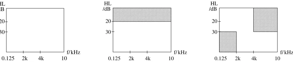
The patient data consists of two sets measured at the Universities of Homburg and Heidelberg, with each consisting of an evaluation of more than 200 ears. The Homburg data represents the training data, the Heidel-berg data is addressed as test data. Both sets are classi-fied to one of the three groups of normal hearing (NH), pantonal (PT), or high frequency (HF) hearing loss, as defined in Fig. 2. For each ear, the TEOAE equipment measured a total of 520 responses, each for a period of 20.48 ms, and calculated two partial averages (labelled A and B) alternatingly over 260 responses each.

Due to the transient nature of the signals, previ-ous work on the qualitative analysis of TEOAE has focused on time-frequency (TF) methods, such as fil-ter banks [5], matching pursuit [6], or discrete wavelet transforms (DWT) [3], whereby a quantitative study w.r.t. the achievable distinction of frequency-specific hearing loss has been performed in [3], based on the DWT.

0.125 2k 4k 10f/kHz /dBHL

20

30

0.125 2k 4k 10f/ kHz /dBHL

20

30

0.125 2k 4k 10f/ kHz /dBHL

20

30

Fig. 2. Characterisation of hearing loss for (left) normal hearing, (middle) pantonal HL, and (right) high frequency HL.

a fixed transform based on a “mother wavelet” from which the transformation coefficients are derived by scaling, translation and sampling. Here, we have cho-sen the Mallat wavelet for which good results have been reported in similar studies [3]. The transform coeffi-cients approximately cover TF tiles as illustrated in Fig. 3 a).

The WP transform is an adaptive transformation sim-ilar to the DWT but with a flexible partitioning of the TF plane. The advantage of this approach compared to the DWT is that the entropy of the transformed data shall be minimised through variable levels of de-composition such that the energy is concentrated in as few coefficients as possible. That minimisation is achieved by the reduction of the concentration accord-ing to Shannon’s entropy [7]. Fig. 3 b) shows a sample WP decomposition.

Based on a parameterisation of the data by the WP, representing the feature extraction of the data, the ap-plication of an SNR-like criterion for the feature selec-tion is conducted which will be described next.

3. FEATURE SELECTION

To quantify and exploit differences in the TEOAE WP coefficients of the three groups of hearing abil-ity within the Homburg data, a signal-to-noise-ratio (SNR) based criterion is invoked. First, the SNR is es-timated for each of the 512 parameters in the TF-plane based on the WPs of the two partial averages, WP_A(n) and WP_B(n),n= 1, . . . ,512. The SNR of thenth co-efficient is (coarsely) estimated by comparing the sum and the difference obtained from the partial averages A and B:

SNR(n) = 20 log₁₀ |WPA(n) + WPB(n)|

|WP_A(n)−WP_B(n)|+ . (1)

This SNR is calculated for all measurements, and for each of the 512 WP coefficients within each of the three hearing ability groups, the distribution is recorded.

The SNR value of a WP coefficient is used to evaluate the separability of any two groups with different hear-ing status. The separability can be assessed indepen-dent of the selection of a specific threshold by means of a socalled receiver operating characteristic (ROC) curve. The area underneath the ROC is a measure for the separability of both groups, and independent of the definition of SNR-thresholds [8].

As single WP coefficients yield a poor separability between any two groups, we pick the coefficient that gives the best separable SNR according to (1) as a starting value and iteratively grow a coefficient setGto improve separability. Further coefficients are added to G from the neighbourhood of surrounding coefficients. Adjacency is defined by edge and corner connections in the TF plane. The iteration is stopped when the ROC does not further improve for the SNR of the coefficients contained inG.

4. SVM CLASSIFICATION

In the following, we briefly explain SVM, [9],[10]. We consider a three class classification problem for the classes defined by the groups NH, HF and PT, starting with an explanation for a two class classification. The training data originates from the Homburg data, while the test data comprises the Heidelberg measurements. The training data is described as a set of training vectors{p_i}_{i=1... M} with corresponding binary labels

Si = 1 for the one class, e.g. NH, and Si = −1 for the second class, e.g. HF. The SVM conducts a clas-sification of a test vectort by assigning a label ˆS by calculating

ˆ

S= sign(f(t)) with f(t) = i

αiSiK(t,p_i) +b.

max-Wavelet Packets

Time

DWT

a) b)

Frequency

Level 1

Level 3

Level 4 Level 2

Frequency

Level 1

Level 3

Time

Level 2 Level 3

Level 4

Fig. 3. TF tiling comparison between a) a DWT and b) a sample WP decomposition.

imising

LD=

i

αi−1₂

i,j

αiαjSiSjK(p_i,p_j) (3)

under the constraints

0≤α_i ≤C and i

αiSi= 0 (4)

withC being a positive constant which weighs the in-fluence of training errors. K(·,·) is called kernel of the SVM. If there is a solution for α_i, a value for b is determined. Usually α_i = 0 for the majority of i and thus the summation in (2) is limited to a sub-net of the p_i, which therefore is called the set of sup-port vectors. There are several commonly used kernels for SVM, which give some flexibility for the underly-ing application. Many implementations of kernels can be found in literature, whereby two popular ones are Gaussian and polynomial kernels. IfK(·,·) is positive definite, (3) and (4) is a convex quadratic optimisation problem, which converges towards the global optimum assuringly. This optimisation can be quite demanding in terms of computation time for real-world problems, and therefore, sophisticated algorithms like sequential minimal optimisation (SMO) [9] are used for the solu-tion.

To find a significant value for the training errorC, a leave-one-out (l-o-o) estimation of the error rate is applied as follows: From the training samples, remove the first example. Train the SVM on the remaining samples. Then test the removed example. If the ex-ample is classified incorrectly, it is said to produce a leave-one-out error. In [9], an approach to estimate the maximum l-o-o error is shown avoiding training

the SVM more than once, which is also used for our study. By changing the value forCstepwise, the mini-mum for the l-o-o error is found determining the SVM classification network. For our application, a Gaussian kernel was used.

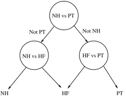
So far, we have described the SVM for only two classes. As we aim at distinguishing 3, we need to define a multi-class method. In [11] a decision directed acyclic graph (DAG) for multi-class SVM is introduced. It is based on an 1-vs-1 classification where the train-ing is conducted for all possible combinations of the classes. Based on a trained SVM classifier for each pos-sible class combination, a binary acyclic graph is used for testing. Fig. 4 shows the decision DAGSVM for our application to the the three classes with different hearing ability.

NH vs HF

Not NH NH vs PT

HF vs PT Not PT

HF PT

NH

Fig. 4. DAGSVM for TEOAE.

5. RESULTS AND DISCUSSION

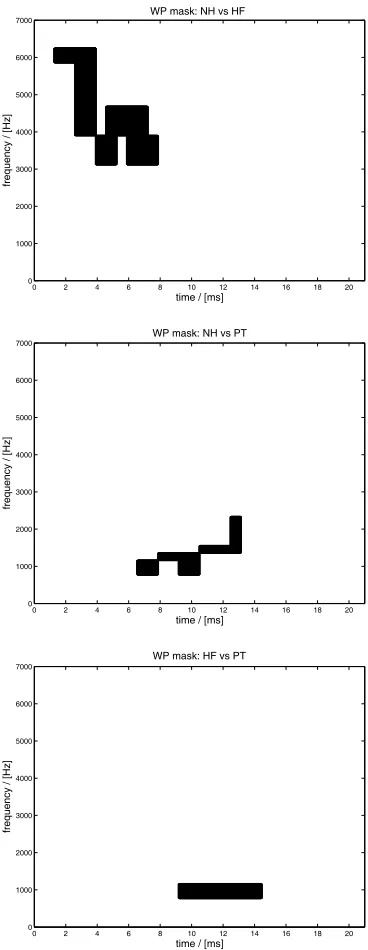
Having described the detection methods and the data used for our system, we present the results in the following. Fig. 5 illustrates the average WP coeffi-cient energy for the training data showing the typical TEOAE properties of high frequencies occurring early and low frequencies appearing late [6]. In Figure 6 the isolated coefficients for each distinction case are shown. They were found by the search procedure based on the SNR criterion explained in Sec. 3 and appear to be rea-sonably located when compared to the average energies in Fig. 5.

Based on the coefficient sets, a SVM classification is conducted for each distinction case using the training data. The test data is analysed by the determined clas-sifiers according to the decision DAG in Fig. 4 yielding the detection rates in Tab. 1 for each class.

group detection rate for test data NH 68.1% HF 74.7% PT 56.4%

Tab. 1. Detection rates yielded by DAGSVM.

allocated correctly by the system which is well in the range of other studies.

E.g in [12], a group of normal hearing is defined by no hearing loss up to 30 dB and a hearing impaired group with a hearing loss over 30 dB. A separation method based on wavelet transforms, ensemble corre-lation, time window design and mean cross-correlation is introduced. The study concludes that by standard analysis 90% of the normal hearing persons and 65% of the hearing impaired patients can be allocated cor-rectly. By applying the various methods, the value for the hearing impaired group is increased by approxi-mately 17% to 83% in that study. Compared to our study we achieve slightly better results when only con-sidering the case NH vs PT, which can be seen as equiv-alent to the case shown in [12]. One could also argue, that our methods lead to a better separation of hearing loss as our threshold for defining the difference between NH and PT was 20 dB, and the worse the hearing loss gets, the weaker the TEOAE appear and therefore the easier it should be to separate them. On the other hand, we achieve the lowest value of 56% for the PT group, which shows that it is easier to separate when clear TEOAE are present, which is more likely the case for a threshold of hearing loss of 20 dB than for 30 dB. Recapitulating it can be said that our approach yields separation results than can well compete with other studies so far.

6. CONCLUSIONS

We have presented a WP analysis of TEOAE that aims at the detection of frequency specific hearing loss. We have motivated the use of TF methods, and pro-posed a method to optimise a set of distinctive WP coefficients. This maximisation represents the input to a SVM classifier for the detection. We used two data sets for training and testing. The validity of the results was verified by a test group. Moreover, the obtained results proved to be competitive when they were com-pared to similar study which also aims at the detection of TEOAE. Therefore, the results appear reasonably robust and encourage frequency specific hearing loss detection via signal processing of TEOAE.

7. ACKNOWLEDGEMENTS

The authors would like to acknowledge Prof. Ulrich Hoppe and Sebastian Hoth of the University of Erlan-gen, Germany, who kindly provided valuable expertise and the data.

REFERENCES

[1] M.S. Robinette and T.J. Glattke, Otoacoustic

Emis-sions: Clinical Applications, Thieme Medical Pub, 2. edition, 2001.

[2] Otodynamics Ltd., Hatfield, Herfortshire, UK, ILO

OAE Instrument User Manual, 5a edition, October 1997.

[3] S. Weiss, U. Hoppe, M. Schabert, and U. Eysholdt, “Wavelet Analysis of Transient Evoked Otoacoustic Emissions for Differential Diagnosis of Cochlear

Hear-ing Loss,” in Asilomar Conference on Signals,

Sys-tems, and Computers, Monterey, CA, November 2001. [4] G. Buller and M.E. Lutman, “Automatic classifica-tion of transiently evoked otoacoustic emissions using an artificial neural network,”British Journal of Audi-ology, vol. 32, pp. 235–247, 1998.

[5] P. Ravazzani, G. Tognola, F. Grandori, and J. Ruoho-nen, “Two-Dimensional Filter to Facilitate Detection

of Transient-Evoked Otoacoustic Emissions,” IEEE

Transactions on Biomedical Engineering, vol. 45, pp. 1089–1096, 1998.

[6] K. J. Blinowska, P. J. Durka, A. Skierski, F. Grandori,

and G. Tognola, “High Resolution Time-Frequency

Analysis of Otoacoustic Emissions,” Technology and

Health Care, vol. 5, pp. 407–418, 1997.

[7] A. Jensen and Anders la Cour Harbo,Ripples in Math-ematics, Springer-Verlag, Berlin, Heidelberg, New York, 2001.

[8] J. A. Hanley and B. J. McNeil, “The Meaning and Use of the Area under a Receiver Operating Characteristic (ROC) Curve,” Radiology, vol. 143, pp. 26–36, 1982. [9] V.N. Vapnik, Statistical Learning Theory, Cambridge

University Press, New York: Wiley, 1998.

[10] C. Bahlmann, B. Haasdonk, and H. Burkhardt, “On-line Handwriting Recognition with Support Vector Machines – A Kernel Approach,” inProceedings of the 8th Int. Workshop on Frontiers in Handwriting Recog-nition (IWFHR), pp. 49–54, 2002.

[11] J. Platt, N. Cristianini, and J. Shawe-Taylor, “Large

Margin DAGs for Multiclass Classification,” in

Pro-ceedings of Advances in Neural Information Processing Systems, NIPS’99, MIT Press 2000, pp. 547–553. [12] A. Janusauskas, L. Sornmo, O. Svensson, and B.

En-gdahl, “Detection of Transient-Evoked Otoacoustic

Emissions and the Design of Time Windows,” IEEE

average WP coefficient energy − normal hearing (Homburg)

time / [ms]

frequency / [Hz]

0 2 4 6 8 10 12 14 16 18 20

0 1000 2000 3000 4000 5000 6000 7000

average WP coefficient energy − HF hearing loss (Homburg)

time / [ms]

frequency / [Hz]

0 2 4 6 8 10 12 14 16 18 20

0 1000 2000 3000 4000 5000 6000 7000

average WP coefficient energy − pantonal hearing loss (Homburg)

time / [ms]

frequency / [Hz]

0 2 4 6 8 10 12 14 16 18 20

0 1000 2000 3000 4000 5000 6000 7000

Fig. 5. Average WP coefficient energy for the dif-ferent hearing ability groups for the training data.

time / [ms]

frequency / [Hz]

WP mask: NH vs HF

0 2 4 6 8 10 12 14 16 18 20

0 1000 2000 3000 4000 5000 6000 7000

time / [ms]

frequency / [Hz]

WP mask: NH vs PT

0 2 4 6 8 10 12 14 16 18 20

0 1000 2000 3000 4000 5000 6000 7000

time / [ms]

frequency / [Hz]

WP mask: HF vs PT

0 2 4 6 8 10 12 14 16 18 20

0 1000 2000 3000 4000 5000 6000 7000