Rochester Institute of Technology
RIT Scholar Works
Theses Thesis/Dissertation Collections
2-1-2008
Estimation and control of the pump pressure rise
and flow from intrinsic parameters for a
magnetically-levitated axial blood pump
Aditi Khare
Follow this and additional works at:http://scholarworks.rit.edu/theses
This Thesis is brought to you for free and open access by the Thesis/Dissertation Collections at RIT Scholar Works. It has been accepted for inclusion in Theses by an authorized administrator of RIT Scholar Works. For more information, please [email protected].
Recommended Citation
Estimation and Control of the Pump Pressure Rise
and Flow from Intrinsic Parameters for a
Magnetically-Levitated Axial Blood Pump
By
Aditi Khare
A Thesis Submitted in Partial Fulfillment of the Requirement for Master of Science in Mechanical Engineering.
Approved by:
Department of Mechanical Engineering Committee
Dr. Steven Day – Thesis Advisor ________________________________
Dr. Agamemnon Crassidis ________________________________
Dr. Steven Weinstein ________________________________
Dr. Edward Hensel – Department Representative ________________________________
Rochester Institute of Technology
Rochester, New York 14623
ii
PERMISSION TO REPRODUCE THE THESIS
MECHANICAL FATIGUE IN A MAGNETICALLY-LEVITATED AXIAL
BLOOD PUMP
I, ADITI KHARE, hereby grant permission to the Wallace Memorial Library of Rochester
Institute of Technology to reproduce my thesis in the whole or part. Any reproduction will not be
for commercial use or profit.
iii
ACKOWLEDGEMENT
Before getting into the thick of the things, I would like to add a few heartfelt words of thanks to
the people who were the most important part of this thesis.
I would like to express my gratitude to Dr. Steven W Day, my thesis advisor. His thoughtful
guidance and insight were most helpful to this work. I would also like to thank the committee
members Dr. Steve Weinstein and Dr. Agamemnon Crassidis for their helpful and healthy
discussion.
Words fail to express my profound gratitude to my beloved parents and siblings, whose love and
blessing is the back bone of my success and confidence. I appreciate my friends Scott, Dave, and
Jeff for their help and a special thanks to Robert Kraynik in Machine Lab, who helped me in
making parts for the test rigs.
Lastly, I am grateful to the National Heart, Lung, and Blood Institute for awarding Grant 1RO1
HL 077085-01A1 to Don Olsen, D.V.M at Utah Artificial Heart Institute, without which this
iv
ABSTRACT
An increase in the number of cardiac patients and a decrease in number of heart donors has
triggered the development of artificial heart pump to support the proper functioning of the heart.
There is also an increase in demand for smaller sized pumps with long term application. All
these factors have stimulated the use of a magnetically-levitated rotary blood pump as Left
Ventricular Assistant Devices. The demand of volume and pressure of blood varies from person
to person. Moreover, the prevention of cannular ventricle collapse at suction, dependence of
pump performance on its inlet, and outlet conditions has necessitated control of the pump. Also,
the available invasive pressure and flow transducers limit the use, due to their low reliability,
periodic calibration, and assembling problem.
In this work, three independent and quantitative non-invasive measurement methods for the
estimation of pump parameters from intrinsic parameters were developed, substantiated, and
compared. The first method used DC motor current and the motor speed as the inputs to the
system. In this method, behavior of brushless DC motor was studied using its working model.
Pump speed and bearing current were the inputs for the second estimation technique. In this
method, pump performance and impeller behavior were continuously monitored in three axes
(X,Y,
θ
). The third method is conceptualized on the output of the Hall Effect sensors, which wereused for sensing the position of impeller, and the pump speed. The behavior of the sensor output
with the impeller position in four axes (X,Y,Z,
θ
) was developed using a real impeller in modelhousing. The data were analyzed in Microsoft Excel 2007 and MATLAB using least square
estimation techniques and Fourier series expansion. An algorithm for each technique was
developed. In addition, the propagation of errors and uncertainties at each step of estimation
v
CONTENTS
Estimation and Control of the Pump Pressure Rise ... i
and Flow from Intrinsic Parameters for a ... i
Magnetically-Levitated Axial Blood Pump... i
PERMISSION TO REPRODUCE THE THESIS ... ii
LIST OF FIGURES ... vii
LIST OF TABLES ...x
NOMENCLATURE ...x
1. INTRODUCTION...1
1.1 Background ...1
1.2 Motivation for the work...3
1.3 Scope ...5
2. CONCEPTUALIZATION ...7
2.1 Technique 1...9
2.2 Technique 2... 12
2.3 Technique 3... 17
3. METHODS ... 22
3.1 Motor –Test Rig ... 24
3.2 Magnetic Bearing Test Rig ... 33
3.3 Waterproof Levitation-Test Rig ... 51
3.4 Mock –Test Loop Rig... 52
3.5 Computational Analysis ... 54
3.6 Theoretical Analysis ... 57
3.7 Uncertainty Analysis ... 58
4. EVALUATION AND UNCERTAINTY ANALYSIS ... 61
4.1 Technique 1... 61
4.2 Technique 2... 66
4.3 Technique 3... 67
5. RESULTS ... 71
vi
5.2 Technique 2... 75
5.3 Technique 3... 76
6. DISCUSSION ... 82
APPENDIX A ... 86
APPENDIX B ... 100
APPENDIX C ... 105
APPENDIX D ... 107
APPENDIX E ... 108
APPENDIX F ... 109
APPENDIX G ... 110
vii
LIST OF FIGURES
Figure 1: Implanted LVAD demonstration [3]. ...1
Figure 2: Sectional view of the pump assembly. ...2
Figure 3: Co-ordinate system with respect to the impeller and the housing [1]. ...2
Figure 4: a. z = 0 position in the pump[8]; b. z Positive in the pump impeller and housing assembly [8]. ...3
Figure 5: Diagrammatic representation of the pump control system. ...4
Figure 6: Diagrammatic representation of the proposed methods. ...7
Figure 7: System model of the BLDCM. ...9
Figure 8: Simulink model of the BLDCM. ... 10
Figure 9: Comparison of motor phase current with speed, varying with time. a: With inductance; b: Neglecting inductance. ... 11
Figure 10: System model for Technique 2. ... 14
Figure 11: Free body diagram of AMB system model. ... 14
Figure 12: Simulink model of the AMB system model. ... 16
Figure 13: Radial displacement and flow variation with time... 16
Figure 14: System model for Technique 3. ... 17
Figure 15: Free Body diagram for axial displacement system model. ... 18
Figure 16: Simulink model of pump for Technique 3... 19
Figure 17: Axial displacement response. a. Frequency= 42 heartbeats per minute (B=10); b. Frequency= 72 heartbeats per minute (B=10); c. Frequency= 42 heartbeats per minute (B=2.5). ... 20
Figure 18: Diagrammatic representation of all relations. ... 22
Figure 19: The motor test-rig, Courtesy of the Blood Pump Lab at RIT. ... 24
Figure 20: Motor rotor, Courtesy of the Blood Pump Lab at RIT. ... 25
Figure 21: a. Solid model of the motor stator; b. Real motor stator, Courtesy of the Blood Pump Lab at RIT. ... 25
Figure 22: Arrangement of the delta configuration in motor coils. a. Coil connections in a three-phase DC motor; b. Overview of the delta connection... 26
Figure 23: Supply current vs. motor torque. ... 29
Figure 24: Phase current vs. motor torque... 29
Figure 25: Motor test-rig including dynamometer... 30
Figure 26: Supply current vs. motor torque. ... 31
Figure 27: Semi-log plot: Supply current vs. motor torque... 32
Figure 28: The HESA test-rig, Courtesy of the Blood Pump Lab at RIT. ... 34
Figure 29: Rotor magnets and their polarity. ... 34
viii
Figure 31: Diagrammatic representation of orientation of the HESs as applied in LVAD... 36
Figure 32: Z=0 positions as defined in the test–rig, Cou rtesy of the Blood Pump Lab at RIT. ... 37
Figure 33 : a. Dial of the Ruby Indicator; b. Ruby Tip Indicator, Courtesy of the Blood Pump Lab at RIT. ... 37
Figure 34: Hall Sensors 1 and 3 (Axial) with variation in θ and the estimated values. ... 39
Figure 35: Hall Sensors 2 and 4 (Radial) with variation in θ and the estimated values. ... 39
Figure 36: HES1 (axial) output variation with respect to X, Y and Z co-ordinates. ... 40
Figure 37: HES2 (radial) output variation with respect to X, Y and Z co-ordinates. ... 41
Figure 38: HES3 (axial) output variation with respect to X, Y and Z co-ordinates. ... 41
Figure 39: HES4 (radial) output variation with respect to X, Y and Z co-ordinates. ... 42
Figure 40: Variation of (V1-V3) in X, Y, and Z co-ordinates. ... 43
Figure 41: Variation of (V1+V3) in X, Y, and Z co-ordinates. ... 43
Figure 42: Variation of (V2-V4) in X, Y, and Z co-ordinates. ... 44
Figure 43: Variation of (V2+V4) in X, Y, and Z co-ordinates. ... 44
Figure 44: Flowchart for calculation of X, Y and Z co-ordinates. ... 46
Figure 45: Histogram for error in x, y,,z and V3. ... 48
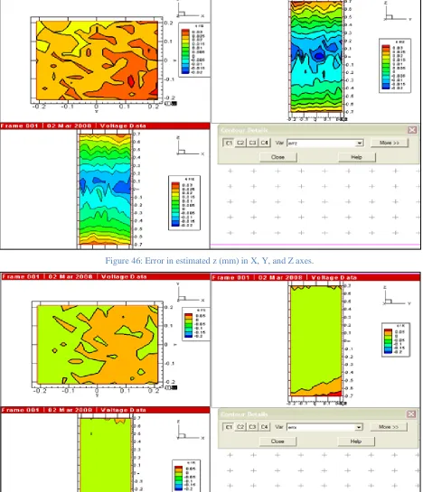
Figure 46: Error in estimated z (mm) in X, Y, and Z axes. ... 49
Figure 47: Error in estimated x (mm) in X, Y, and Z axes. ... 49
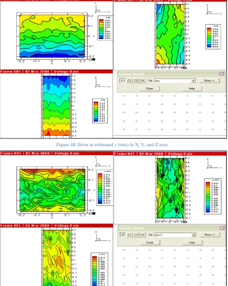
Figure 48: Error in estimated y (mm) in X, Y, and Z axes. ... 50
Figure 49: Error in estimated V3 (volts) in X, Y, and Z axes. ... 50
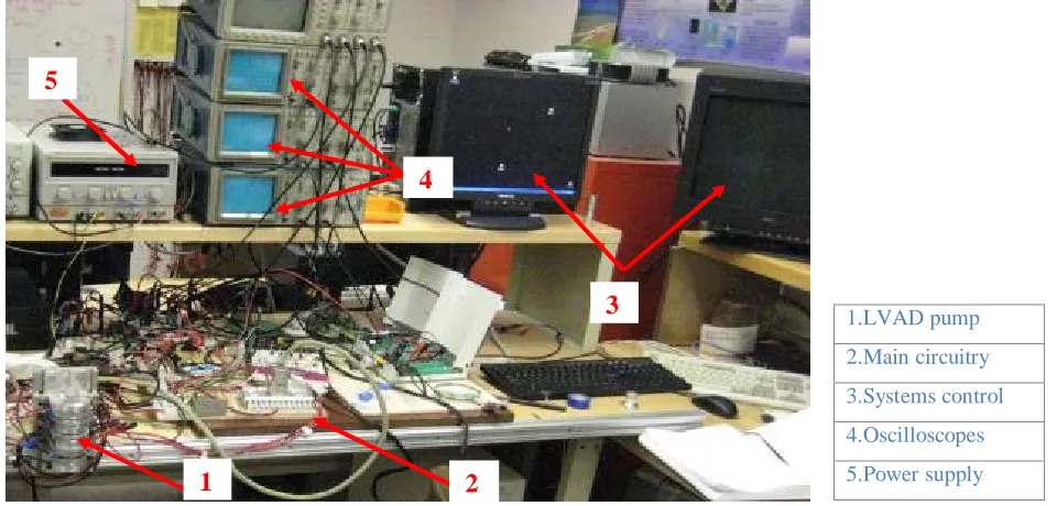
Figure 50: Complete LVAD system, Courtesy of the Blood Pump Lab at RIT. ... 51
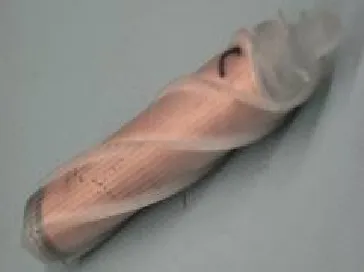
Figure 51: Impeller, Courtesy of the Blood Pump Lab at RIT. ... 51
Figure 52: Levitation test-rig, Courtesy of the Blood Pump Lab at RIT. ... 52
Figure 53: Mock test loop, Courtesy of the Blood Pump Lab at RIT. ... 53
Figure 54: Characteristics curve from CFD results. ... 54
Figure 55: Graphical comparison of the estimated values with computational values of Ф as a function of Ψ. ... 56
Figure 56 : Graphical comparison estimated ∆P values with computational ∆P as a function of applied torque. ... 57
Figure 57: Flowchart for calculation of ∆P and Q by Technique 1. ... 61
Figure 58: Flowchart for calculation of P and Q by Technique 3. ... 67
Figure 59: Motor torque as a function of supply current. ... 72
Figure 60: Pump ∆P as a function of applied torque and pump speed. ... 72
Figure 61: Estimate flow using pump performance curve. ... 73
Figure 62: Compare experimental and estimated ∆P with the uncertainty limits. ... 73
Figure 63: Compare experimental and estimate pump flow with uncertainty limits. ... 74
Figure 64: Pressure distribution across the pump at displaced radial positions [15]. ... 75
Figure 65: Bearing current vs. pump differential pressure at constant radial displacement. ... 75
ix
Figure 67: Estimate flow using pump performance curve for VCC = 5volts. ... 77
Figure 68: Compare experimental and estimated ∆P with the uncertainty limits for VCC = 5volts. ... 78
Figure 69: Compare experimental and estimated pump flow with uncertainty limits for VCC = 5volts. ... 78
Figure 70: Axial displacement of the impeller as a function of the Hall Sensors output for VCC = 5.45volts. ... 80
Figure 71: Estimate flow using pump performance curve for VCC = 5.45volts. ... 80
Figure 72: Compare experimental and estimated ∆P with the uncertainty limits for VCC = 5.45volts. ... 81
Figure 73: Compare experimental and estimated pump flow with uncertainty limits for VCC = 5.45volts. ... 81
Figure 74: Extrapolated view of impeller rotation along x axis. ... 82
Figure 75: Flow and pressure characteristics with cannula resistance effects [5]. ... 89
Figure 76: Deposition of blood particles in dead-water areas at the gap of a connector-tubing assembly [5]. ... 90
Figure 77: Relationship between left ventricular systolic pressure and peak motor current in a mock circulatory loop[25]. ... 93
Figure 78: Relation between pump flow, power and motor rpm [26]. ... 95
Figure 79: Flowchart to summarize the proposed method in the article. ... 96
Figure 80: a. Graph between head pressure and pump flow; b. Graph between the impeller position and pump flow; c. Graph between the impeller position and head pressure [2]. ... 96
Figure 81: Basic concept of a BLDCM. ... 100
Figure 82: a. One switch position for a three-phase delta-connected BLDCM, 134 [9]; |b. Three-phase delta connection for six coils stator [9]. ... 102
Figure 83: Torque production in a delta connected three phase DC motor [25]. ... 104
Figure 84: Supply current vs. motor torque, at different speeds for Technique 1. ... 105
x
LIST OF TABLES
Table 1: Types of relation and their respective test-rig. ... 23
Table 2: Constants for the variation with rotation angle (θ). ... 38
Table 3: Constants for the estimation of voltage output for HES 1 and HES 3. ... 45
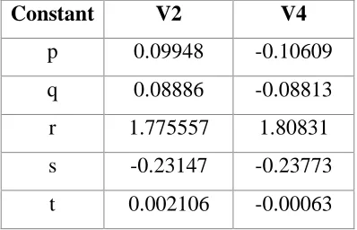
Table 4: Constants for the estimation of voltage output for HES 2 and HES 4. ... 46
Table 5: Uncertainties considered while estimating the pump flow and the delta pressure by Technique 1. ... 62
Table 6: Uncertainties considered while estimating the pump flow and the delta pressure by Technique 3. ... 68
Table 7: Results of Technique 1. ... 71
Table 8: Results of Technique 3 with Vcc = 5volts. ... 76
Table 9: Results of Technique 3 with Vcc = 5.45volts. ... 79
Table 10: Commutation sequence for a three-phase BLDCM, with delta connection. ... 103
Table 11: Percentage variation in Hall Sensor output with angle ‘θ’. ... 107
NOMENCLATURE
AMB Active Magnetic Bearing
BLDCM Brushless DC Motor
CFD Computation Fluid Dynamics
HES Hall Effect Sensor
HESA Hall Effect Sensor Array
LVAD Left Ventricular Assistant Device
MBTR Magnetic Bearing Test Rig
PMB Permanent Magnetic Bearing
PWM Pulse Width Modulation
VZR Virtual Zero Run-out
1
1. INTRODUCTION
1.1 Background
Left ventricular Assist Device (LVAD) - a mechanical pump connected to the human heart
(Figure 1) - assists the left ventricle or the natural heart. Earlier LVADs have been used as a
“bridge-to-transplant” - an aid to the weakened heart until the availability of appropriate donor
[image:12.612.201.487.281.516.2]heart. Recently, LVADs are focused on providing a permanent solution to a sick heart.
Figure 1: Implanted LVAD demonstration [3].
For decades, centrifugal pumps and rotary pumps are being studied and used as LVADs.
Recently, more advanced systems are under development. The specific LVAD, which is under
development at Rochester Institute of Technology, is a magnetically-levitated axial blood pump.
The main parts of this LVAD (Figure 2) are two active electromagnetic bearings (AMB); four
permanent magnet (PM) rings (in pair sandwiching the AMBs); a brushless DC motor
(BLDCM); and a magnetic impeller. The impeller is suspended by a magnetic force, which acts
as a frictionless bearing. The AMB keeps the impeller stable in radial direction. The two PMs Natural Heart
LVAD
2
Figure 2: Sectional view of the pump assembly.
provide rigidity to the impeller; one at the center provides stiffness in axial direction and other at
the rear end adds stiffness in radial direction. The pump impeller is a hollow tube with impeller
blades on it. The tube contains all the magnets; motor, AMB, Hall, and PMB magnets.
The impeller has six degrees of freedom, which are described in Figure 3. The zero co-ordinates
of X and Y axis are defined by the concentric center of impeller and housing.
3
(a) (b)
Figure 4: a. z = 0 position in the pump[8]; b. z Positive in the pump impeller and housing assembly [8].
The zero co-ordinate of the Z axis is defined by the relative position of the hall sensor (in the
housing) to the hall magnet (in the pump), shown in Figure 4.
The LVAD circulates clean blood into the whole body to support the functioning of the natural
left ventricle. The cardiac output of a healthy human heart at rest, with 70 heartbeats per minute
is 5.3 liters per minute [7]. This value differs from person to person and also varies with the
physiological requirements. The LVAD under study is designed to operate at 6000 revolutions
per minute and pump about 6 lpm (0.0001 m3/sec) of blood at a pressure of about 50 mmHg (6666.1195 pascal), in order to replace a healthy left ventricle of the human body.
On an average, variation up to 20% in the blood flow and pump differential pressure is
considered acceptable, in any situation. The available non-invasive parameter estimators for
centrifugal and axial pumps, works almost in the same range. The best estimation for the axial
pump using auto-regressive exogenous models [6] is 1.66 lpm (31% of 5.3 lpm) for pump flow
and 12.9 mmHg (25.8 % of 50 mmHg) for pump pressure head.
1.2 Motivation for the work
Currently, LVADs are focused on long term applications. Ideally, LVADs can maintain the
quality of life while a patient goes through various physical activities like walking, climbing,
sleeping, eating, running, etc. which vary the cardiac output in the range of 4 lpm to 10 lpm and
the developed pressure in the range of 50 to 150 mmHg. Also, with time, the sick left ventricle
itself might undergo change after surgery and become either better or worse, which necessitates
the monitoring of developed pump pressure and pump flow. Moreover, a precise and adequate
4 pressure head across the pump. This necessitates the physiological control of LVAD [4], which
requires the continuous monitoring of the developed pressure and pump flow of the LVAD.
Theoretically, a non-pulsatile continuous pump flow and speed can be regulated by a single
knob, so measurement [5] like pump flow or delta pressure head is not required. However studies
show there are cases where problem arose during suction at high speed due to change in
circulatory conditions, for example, heartbeat rate, peripheral resistance change or arrhythmia
[2]. Thus a real time monitoring system is needed to prevent suction or back flow in LVAD.
During systole, the heart contracts and forces the blood in the chambers onwards. The volume of
blood filled in the heart chambers during dilation, known as preload is directly related to the
stretch of the myocardial muscles. According to the Frank-Starling Law, the output of the heart
ventricles is dependent on the preload condition [7]. At the end of the systole, the ejection stops
when the ventricular pressure, known as afterload, developed by the myocardial contraction falls
below the arterial pressure. The amount of the blood pumped by the left ventricle would be same
as the blood returned from pulmonary vein, i.e. the cumulative amount of blood returned from all
the tissues and organs to the heart. This volume of generated blood satisfies the blood demand of
the body.
The specific LVAD under study is an impeller-based axial pump. Unlike positive displacement
pumps, the output of this pump is dependent on the inlet and outlet pressure values. This needs to
be controlled to satisfy the physiological demand of the human body, which requires real time
values of the pump flow and the pump pressure as the feedback signals.
5 The measurement of these feedback signals using implanted sensors is uncomfortable to the
patient because of the wirings through the body. In this study I propose three non-invasive
measurement methods for these feedback signals. The main advantages of non-invasive
measurement techniques are:
• More reliable as compare to the available pressure and flow transducers for long term application (>20 years).
• Reduce the problem of regular calibration and maintenance of the implanted sensors.
• Reduce the risk of thrombus formation and infections due to the implantation of sensors,
by reducing the corners (regions prone to fluid accumulation) in the 1pump housing.
• Minimize the size of the implanted LVAD system. Ultrasound and electromagnetic flow
probes are often used to monitor pressure; however these sensors are sometimes too
bulky for implantation [6].
• Reduce additional power consumption [6].
• Overcome the requirements of implanted sensors which do not react with the blood.
• Minimize the use of sensors and reduce total cost of the system.
In this paper, non-invasive measurement refers to the measurement of pump performance
without the use of additional sensor, blood contacting device, or intrusion of any extra wire in the
body.
Research has been going on for about last three decades on the non-invasive monitoring of
pulsatile total artificial heart and assist systems with success achieved on centrifugal pumps
applications [5]. However, the pump under study is an axial pump and is magnetically levitated.
All above factors motivated me to work on the parameter estimation techniques for the pump,
which is under development at Rochester Institute of Technology.
1.3 Scope
This thesis comprises of three estimation techniques for the non-invasive and sensorless
measurement of the pump performance. Basic study of BLDC motor, magnets, and
impeller-axial pump have been done with dependence of their respective parameters characterized. Test
6 results were analyzed and uncertainty analysis was performed to compare the reliability of the
three methods. Codes were developed to compute the uncertainty using Microsoft Excel
spreadsheets and MATLAB.
The test results and analysis are distinct for this pump with given specifications. Coefficients of
the relations might change with the change in the parameters (impeller blade angle, number of
coils in motor windings, etc.) of the pump, but the basic form of relation would remain same. A
graphical user interface (GUI) was developed in MATLAB, to estimate the desired parameters
based on the designed estimators. This will facilitate future work. The derived equations for each
technique were also programmed in Microsoft Excel 2007, which can be used for other such
applications.
This estimator is designed to measure pump flow and differential pressure head with an accuracy
7
2. CONCEPTUALIZATION
The designed estimator, focused on the non-invasive measurement techniques uses the intrinsic
parameters of the LVAD and control unit to estimate the pump flow and differential pressure
across the pump. Based on the characteristic properties of the pump, motor and the AMB, I have
suggested three estimation methods. The diagrammatic overview of all the different techniques is
represented in Figure 6.
Figure 6: Diagrammatic representation of the proposed methods.
Technique 1 is based on the hypothesis that motor current is directly proportional to the motor
torque (Appendix B) and differential pump pressure, and flow would depend on the pump speed
and applied torque (Section 3.5). Using this approach, relation between the motor current, pump
8 pressure was estimated by using performance curve characteristics with pump flow and pump
speed as the inputs.
Technique 2 evaluates the developed pressure head by measuring the impeller position
variability in the radial direction. It is based on the hypothesis that during flow, the developed
pressure gradient shifts the impeller in the radial direction. To neutralize this flow effect and
maintain the centralized position of the impeller, a counteracting force is generated at the
electromagnetic bearing. This counteracting force is directly related to the current supplied to the
bearing coils.
Technique 3 estimates the developed pressure head by means of impeller position variability in
axial direction. The basis of this approach is that the pressure rise across the pump results in the
impeller axial shift. This axial shift measures the differential pressure across the pump. In this
LVAD system, permanent magnets are used to avoid dislocation of the impeller. They provide
stiffness to the impeller in the axial direction and Hall Effect Sensors (HESA) sense the axial
shift.
The basic architecture of all the techniques can be visualized by designing their system models.
The idea in this study is not only to encapsulate the complex aspects of the design, but also to
focus on the interaction of the subsystems. This will help in understanding the reliability and
9
2.1 Technique 1
Technique 1 uses three phase BLDCM characteristics as the inputs to estimate the pump
parameters. The construction and working of the BLDCM is described in Appendix B. It is an
electromechanical system and its system model can be represented as:
Ea : Voltage applied across the armature (volts)
Eb : Back EMF induced by armature winding rotating
in magnetic field (volts)
Ra : Armature resistance (ohms) La : Armature inductance (henry) ia : Armature current (ampere)
w : Angular velocity of the motor (rad/sec)
τ : Torque developed by motor (Nm)
The resistance value as measured is 0.2 Ω for a coil.
The inductance value of a coil is calculated as:
L = µc2Al-1
where,
µ = Kµ0; K is the relative permeability (K=1 for air) and µ0 is the absolute permeability c : Number of coils in a coil = 21
A: Cross sectional area of the wire. Diameter of the wire = 0.511mm
l : Length of the solenoid = 3.175×105 cm Substituting the values, L = 0.0715923 H
Equating the voltage across the loop gives:
Eୟ Rୟiୟ Lୟୢ୧ୢ୲ Eୠ 0 …Eq.1.a
10
Substituting Eb from Eq.(51) in Appendix B, the equation reduces to:
Eୟ Rୟiୟ Lୟୢ୧ୢ୲ Kଶw 0 …Eq.1.b
The above equation is a first order linear differential equation, relating ia as a function of Ea & w.
Let τୟ
ୖ ; known as the armature current time constant.
Eq.(1.b) in terms of time constant reduces to:
τୟୢ୧ୢ୲ iୟ ୖଵEୟ Kଶw …Eq. 2.a
i.e. iୟ1 τୟD ଵ
ୖEୟ Kଶw …Eq. 2.b
11
(a)
(b)
Figure 9: Comparison of motor phase current with speed, varying with time. a: With inductance; b: Neglecting
12 The supply voltage is considered constant. Variation of pump speed and armature current (phase
current), along with the effect of inductance are studied here (Figure 9).
As shown in Figure 9a (L = 0.0715923 H) and Figure 9b (L = 0), the effect of inductance is
negligible. Thus inductance is neglected for further analysis. To make the task easier, the
characteristics of the motor are derived at steady state. In addition, due to the high rate of change
of phase current (three times the motor speed), the variation of the supply current with the
developed torque is studied. At an instant the supply current would be the sum total of all the
phase currents and would be more stable as compared to individual phase currents.
The model shows the variation of the motor torque (τ) with the variation in the phase current and
the motor speed. The pump outputs (flow and the differential pressure across the pump) depend
on the pump input, which is the motor torque. This relation is derived later in section 3.5.
2.2 Technique 2
As discussed, the second technique uses the AMB’s supply current used to magnetically levitate
the impeller as an input to estimate the pump parameters. An AMB consists of four
electromagnets, two power amplifiers to supply equal bias current to two pairs of diagonally
opposite electromagnets, and a controller to direct and control the current through the coils.
An electromagnet is usually a solenoid with an iron core. The magnetic field generated in an
electromagnet is defined by:
B = µnI …Eq.3
where,
B = Developed magnetic field (T)
µ = Kµ0; K is the relative permeability and µ0 is the absolute permeability n : Number of the coils
I : Current in the coil (ampere)
13 The system model of the complete pump unit is very complex. Thus for simplification, separate
working models of the system were designed and classified on the basis of degrees of freedom of
the system. In this case, AMBs are considered responsible for the radial displacement of the
impeller. Thus the system model with the forces in only radial direction was derived. The
following assumptions are made while deriving this system model:
• The impeller is assumed to have only one degree of freedom (Figure 10).
• No torsional torque on the impeller.
• Damping effects due to fluid are included / distributed equally with damping coefficient
of both AMBs.
• The z axis of the pump is horizontal, i.e. longitudinal axis is parallel to the ground surface.
• The impeller is assumed to be always parallel to z axis, i.e. rotation along x, y and z axis
is not considered in this model. As rotation along z axis wouldn’t affect the force vectors
and the rotation along x and y axis, it will complicate the problem.
• The impeller displacement in the front and rear end of the impeller are assumed to be the
same.
The intricacies can always be added to the present model, and it can be more refined to real time
situations. As discussed earlier, the motive is to achieve the basis to design experiments for the
related study.
The forces due to the generated magnetic field by the AMBs are represented as a combination of
the spring and the dampers. The values of the spring constants and the damping coefficients are a
function of the generated magnetic field in the AMB, which is in turn a function of the supply
current to AMBs. Therefore, the spring and damper coefficients are a function of the supply
current to the AMBs. There is also a constant radial stiffness due to the permanent magnets of
14
Figure 10: System model for Technique 2.
where,
x
F : Displacement in the radial direction K1, B1 : Stiffness and damping due to AMBs K2 : Stiffness due to motor magnets m : Mass of the impellermw(t) : Mass of the flowing water in upper half of the pump
= Qt
ସD୦୧ଶ D୧୫୮ୣ୪୪ୣ୰ଶ
where,
Dhi : Housing inner diameter
Dimpeller :Impeller outer diameter (excluding blades)
Q(t) : Instantaneous flow
The free body diagram of the model can be represented as:
15 The model is analyzed using D’Alembert’s principle, according to which the sum of the
differences between the forces acting on a system and the time derivative of the moments of the
system itself along a virtual displacement consistent with the boundary conditions of the system,
is zero. Applying this principle to the above model reduces to:
Kଵx Bଵx Kଶx Kଵx Bଵx mx mg mwtg …Eq.4.a
Rearranging terms, the equation reduces to:
2Kଵ Kଶx 2Bଵx mx mg mwtg …Eq.4.b
The state space model of the above equation can be written as:
ଵ
ଶ = A ! xଵ
xଶ" + Bu
and, Y = C !xxଵ
ଶ" + Du
where,
A $ିሺଶ0భାమሻ 1 ୫
ିଶభ ୫ %
B 0
1 m& C (1 1)
D (0)
ଶ ଵ & xଵ xF
u = mg + mw(t)g
The above derived system model is a linear model. It shows that as the mass of the impeller is
constant, the only driving force for the radial displacement of the impeller is the force exerted by
the fluid represented by mw(t). To predict the variation in radial displacement with respect to
variation in the differential pressure, the approximate values of the coefficients are assumed and
simulated (Figure 12).
16
Figure 12: Simulink model of the AMB system model.
The flow is assumed to have sinusoidal variation. The radial displacement shows good variation
with the flow. The response in radial displacement showed a good variation with the flow
(Figure 13).
The flow considered is high and so is the radial displacement. This may be due to error in
assuming the constants. However the zest is that the variation in radial displacement is strongly
17 related to the variation in the flow. Since in the pump flow, differential pressure and pump speed
are mutually related (Section 3.5) it can be verified that there is a relation between AMB current
and pump flow or i.e. the differential pressure across the pump.
2.3 Technique 3
This technique is based on the simple pressure - force relation with displacement, for a constant
mass. The critical point in this LVAD system is its uniqueness in variation of its axial stiffness.
The system model of the pump in the axial direction can be easily represented by a
spring-damper mass system with an external variable force (Figure 14). Damping is added to include the
effect of viscosity of the fluid flow.
Figure 14: System model for Technique 3.
where,
K : Axial stiffness (N/m)
B : Damping coefficient due to viscosity of fluid (Nsec/m)
z : Axial displacement (m)
m : Mass of the impeller (Kg)
∆P : Differential pressure across the pump which varies with time (Pascal)
A : Cross sectional area of the impeller (m2)
The system model design is based on the following assumptions:
• The displacement of impeller is considered only in one degree of freedom (Figure 15).
• Rotation of the impeller is not considered as it does not affect any force vector in this direction.
• The z axis of the pump is horizontal, i.e. longitudinal axis is parallel to the ground surface
(as in section 2.2). Thus effect of gravity is neglected.
K
B
z
18 • The impeller is always parallel to the z axis. Thus the force is assumed to exert on a
constant area.
All the forces on the impeller in this system model are shown in Figure 15.
Figure 15: Free Body diagram for axial displacement system model.
Using D’Alembert’s principle, the above free body diagram reduces to:
mz Bz Kz ∆Pt 0 …Eq.6
The equivalent state space model can be represented as:
ଵ
ଶ = A ! xଵ
xଶ" + Bu
and Y = C !xxଵ
ଶ" + Du
where,
Aଵ 0 1
K m& B m& Bଵ 1 m& 0
C (1 1) D (0) ଶ ଵ & xଵ
-u = ∆P(t).A
The derived model is a linear system and shows the relation between the differential pressure
across the pump and the axial displacement of the impeller. To investigate the effect of time
response in the axial displacement with the change in differential pressure, the model is
simulated in MATLAB (Figure 16).
19
Figure 16: Simulink model of pump for Technique 3.
The differential pressure is assumed to have a sinusoidal variation and the axial displacement
response is plotted (Figure 17).
20
(b)
(c)
21 The derived model is a linear system and shows the relation between the differential pressure
across the pump and the axial displacement of the impeller. To analyze the time response in the
axial direction with respect to change in the differential pressure, the model is simulated in
Simulink (Figure 16). It is also used to study the significance of the damping coefficient on the
system performance.
To simulate the developed pressure in the heart pressure, a square of frequency 72 heartbeats per
minute is selected as an input to the model. It is also simulated at a lower frequency of 42
heartbeats per minute in order to study the time response in axial displacement with respect to
the frequency change.
As seen from the Figure 17a and Figure 17b, the variation in the axial displacement is very
sensitive to the variation in the differential pressure across the pump and insensitive to the
change in frequency. Moreover, the delay time (50% of the final value) for the axial
displacement signal is only few milliseconds, which shows an effective response in the output
signal variation.
The change in the values of the damping coefficients in the system model is quite significant
when a square wave is considered as an input. The variation in the settling time and the peak
overshoot are affected significantly by changing the damping coefficient value from 2.5 (Figure
17c) to 10 (Figure 17a and 17b). But no such variation is seen when a sine wave at the same
frequency was used as the input signal (not shown in the report). Even with no damping, the sine
wave shows no oscillation.
In the natural heart the pressure variation is neither a pure sine wave nor a square wave, rather it
can fairly be defined as a combination of both, with significant sine variation. Therefore, in
22
3. METHODS
Simple parametric relations were derived to develop the three discussed estimation techniques.
These relations were classified into three groups: theoretical, simulation, and experimental. One
relation was a known fact; however, its coefficients were derived, two relations were derived by
computational analysis, and the rest were quantified by various sets of experiments. All the
different kinds of experiments performed can be summarized and represented by a block diagram
(Figure 18).
Figure 18: Diagrammatic representation of all relations.
As illustrated in the above figure, the relations required to derive and accomplish the goal are:
1) Motor phase current and motor torque.
23
3) Differential pressure across the pump and electromagnetic bearing current.
4) Differential pressure across the pump and the radial displacement of the impeller.
5) Differential pressure across the pump, pump flow rate and pump rotational speed.
6) Differential pressure across the pump and the axial displacement of the impeller.
7) Differential pressure across the pump and the motor speed.
The designs of experiments were based on the availability of resources and time. To facilitate the
process of design, the relations described above were further classified.
Table 1: Types of relation and their respective test-rig.
# Description of Relation Type Test-rig/Instrument Name
1) Motor phase current and motor torque Experimental Motor-test Rig
2) Hall sensor output and axial displacement of
the impeller Experimental MBTR
3) Differential pressure across the pump and
electromagnetic bearing current Experimental WLTR
4) Differential pressure across the pump and the
radial displacement of the impeller Experimental Mock Loop Rig
5) Differential pressure across the pump, pump
flow rate and pump rotational speed Simulation CFD
6) Differential pressure across the pump and the
axial displacement of the impeller Theoretical Theory based analysis
7) Differential pressure across the pump and the
24 3.1 Motor –Test Rig
The test-rig to measure the performance of motors was designed using SolidWorks 2006 by the
Blood Pump Lab team. I machined the parts in the machine shop at Rochester Institute of
Technology. The main parts of test-rig are demonstrated in Figure 19.
Figure 19: The motor test-rig, Courtesy of the Blood Pump Lab at RIT.
The BLDCM under study has four poles and three phases. It is a permanent magnet synchronous
motor, which has magnets on the rotor and coils on the stator. The current was electronically
switched through the coils in a manner similar to a conventional DC motor via commutator and
brushes.
It is a quadrature motor, which has a two pole magnet rotor as shown in the Figure 20. The rotor
was slip fit on the carbide shaft with diameter 3/16″, length 6″, and width 0.814″, which equals
the width of the stator windings. For proper positioning and adding strength to the motor, glue
was used between the rotor magnets and the shaft. In the test rig this shaft was supported by
SR3SS, Barden miniature bearings on both the ends.
25
Motor Coils Stator Coils
Figure 20: Motor rotor, Courtesy of the Blood Pump Lab at RIT.
The motor stator has six coils (Figure 21), two per phase. It was made of iron and pressed in
pillow block. Each stator leg was wrapped with 20 ±1 turns of MW-MC 5516-022 24 HTAIH
Natural 792 feet/spool, class 35 with thermal rating 200 C wire. The coils were winded in a
particular direction, either clockwise or counter-clockwise, and were checked number of times
for continuity.
(a) (b)
Figure 21: a. Solid model of the motor stator; b. Real motor stator, Courtesy of the Blood Pump Lab at RIT.
A US digital optical encoder (HEDS–EM1/HEDS-9140-A00), with hub disk (-500-250-1-I) was
mounted on one end of the rotor shaft (outboard of the bearing) to acquire the required rotational
motor speed. CA-3132 - FT, a five pin finger latching cable power the encoder and measure the
output. A constant voltage of 5V was supplied to the encoder assembly. The sensor produced
digital quadrature outputs and was measured from channel A of the encoder, with Omega
26
The other end of the shaft, coupled with another standard DC motor was used as a variable load
to the BLDC motor and referred to as the brake motor from this point forward. The brake motor
was connected to variable pot resistors (0-20Ω), which varied the load on the DC motor and
torque on BLDCM. The DC motor was supported by ball bearings, but was restrained to rotate
about an extended arm to measure load on the motor. Futek load sensor LSB200 (L2357),
miniature S beam load cell unit (includes sensor and the cable interface between the sensor and
the amplifier) with the Futek amplifier module CSG110 (JM-2AD), measured the load. The load
cell assembly was calibrated at a constant supply voltage of 12V. The DC voltage output was
measured by a multimeter. Force was calculated using the module calibration equation and then
the torque was calculated as the product of the measured load and the length of the motor arm.
An electronic inverter was used to convert DC bus voltage to appropriate current waveforms
needed to drive the BLDCM [9]. The driver supplied current to windings for producing an
adequate interaction between the electric and magnetic field and for generating torque in the
desired direction. The six stator coils were connected in delta (▲) configuration (Appendix B).
Figure 22a shows the arrangement of coils using this configuration; A, B and C are the three
phase for the power supply. Figure 22b shows the same connection specifying the delta
connection.
Figure 22: Arrangement of the delta configuration in motor coils.
a. Coil connections in a three-phase DC motor;
b. Overview of the delta connection. (b)
27 Several motor drivers (electronic commutator and controller) were employed to test the
performance of the motor. Allegro 8904, a three-phase BLDCM driver cum controller with
control chip 8904VIP10, was used with the Y connection (Appendix B) in the motor coils. This
controller has self-contained back EMF sensing [A8904], motor startups, and running
algorithms. It can be programmed for precise motor speed control, however this driver cum
controller failed to perform well at high speeds (6000 rpm and above). The problem to reproduce
results and high speed variations were encountered at higher speeds. The motor were
characterized at 6000 ±1000 rpm as the LVAD was designed to give the required flow at 6000
rpm only.
Electric Fly SS-8 Brushless ESC, Silver series was the second controller used. This controller
has a Safe Start program [SS-8 Manual]. National Instruments CB-68 LP Data Acquisition Board
was used as an interface between the controller and the computer. The motor was controlled by a
LabVIEW 8.2 Pulse Width Modulation (PWM) algorithm. This PWM program adjusted the
frequency and duty cycle of the square wave required by the speed controller. The preferred
frequency for remote sensing systems 50Hz [10], was used as input frequency for the tests. The
speed of the motor can be controlled either by changing the supply voltage (6-12V) or by
changing the duty cycle from the LabVIEW program. This controller also worked fine at low
speeds and no loads. But at higher speed @5000 rpm, with a slight increase in load, the motor
encountered stalling problems. This might be because SS-8 had a low voltage cut-off, which was
preset and non programmable.
Castle Creations Phoenix 25 Speed Controller performed better than other motor controllers
tested, which made it an obvious choice for my work. The motor coils were connected in delta
connection, to power with Phoenix 25. The controller was connected to a CP68 LP Data
Acquisition Board and used a default frequency of 50Hz for the PWM. The connections were
same, as described for SS-8. This is the only controller that has been successfully used in full
pump assemblies. All of the data presented here are for the Phoenix 25 Speed Controller.
Honeywell Micro Switch Current Sensors, CSLA2CD were used to measure the phase current
28 wire and a power supply of 8V. The calibrated equation to estimate the current from the output
voltage of current sensor is:
Current (A) = 4.924 × Output Voltage – 19.832 …Eq.8
An algorithm was developed using LabVIEW to acquire the outputs from these sensors. These
outputs were taken using four channel Tektronix oscilloscope TDS 420. However, due to
unavoidable noise, the readings were only taken by oscilloscope for last two sets of experiments.
Phase current refers to the current through the coils, and the loop current refers to the current
supplied by the controller to phase A, B, and C. The magnitude of the phase current was taken as
a root mean square value of the amplitude of the phase (AC) current wave. The supply current
and voltage were directly measured from the power supply.
The controller, load cell, and current sensors were powered by two separate units of Shenzhen
Mastech DC Power Supply HY3003-3. CP68 LP Data Acquisition Board was used to power the
optical encoder with 5V, from the computer.
The experiments were performed using various combinations of the motor parameters. Readings
(data sets) at constant rpm and supply voltage were recorded to analyze the variation of current
with the change in load. Constant speed was achieved by varying the duty cycle in the LabVIEW
program. The load on the DC motor was varied by changing the resistance of the brake motor.
The variation in developed torque with supply current and phase current were analyzed.
The motor was also tested at no load condition, i.e., without the brake motor. The results were
analyzed in Microsoft Excel 2007 using the linear regression method. The statistical model used
in estimation was based on the graphs of the results, and were finalized by checking the lowest
sum of squared estimated errors. The estimation of torque from supply current and phase current
29
Figure 23: Supply current vs. motor torque.
Figure 24: Phase current vs. motor torque.
0 0.002 0.004 0.006 0.008 0.01 0.012 0.014 0.016 0.018 0.02
0 0.1 0.2 0.3 0.4 0.5 0.6
M
o
to
r
T
o
rque
(
N
m
)
Phase Current (Amp)
4000 5000 6000 Estimated
30 Analyzing above graphs, the variation in torque with respect to the phase current and the supply
current were found identical. This is substantiated by the fact that the electronic commutator
used to drive the motor divides the supply current equally in all the three phases of the motor.
Due to feasibility in measurement of supply current and less estimated uncertainty in torque
estimation only the graphs of torque versus motor supply current were used for further analysis.
The relation between the phase current and the torque, and between the supply current and the
torque derived using above graphs are:
Tmotor = 0.0224 ip + 0.00376 …Eq.9 Tmotor = 0.00338 I + 0.00503 …Eq.10
where, Tmotor : Torque in the motor (Nm)
ip : Phase current (A) I : Supply current (A)
The uncertainty in the estimated values using Eq.(9) and Eq.(10) was 25% and 20% respectively.
This was accounted mainly due to uncertainty in torque measurement. So, a Magtrol make,
Hysteresis Dynamometer (Figure 25) (model: HD-100-8N), was used and operator errors were
reduced by automating the data monitoring in LabVIEW.
Figure 25: Motor test-rig including dynamometer.
With the improvement in the rig, and ease in taking the data points, measurements were recorded
for motor speed ranging from 2000 rpm to 7000 rpm with span of 1000 rpm; and supply current
31 date of data collection was not resolved. The variation of torque for BLDCM with respect to
supply current resulted as motor speed dependent, and was no more a linear variation. The
results are shown in Figure 26. Torque was estimated as the fourth order polynomial function of
the current, where the coefficients of the equation are a function of the motor speed. The
uncertainty in data measurements are not shown in the graphs below to avoid confusion.
Detailed graphs at each speed with calculated uncertainty are included in Appendix C.
Figure 26: Supply current vs. motor torque. 0 5 10 15 20 25 30 35 40 45
0 1 2 3 4 5 6 7
M o to r T o rque ( N -m m )
Supply Current (A)
Supply Current vs. Motor Torque
32 The relationship of the torque and current from the above graphs is:
Tmotor = a I4 + b I3 + c I2 + d I + e …Eq.11
where, Tmotor : Torque in the motor (Nmm)
I : Supply current (A)
a : 2.45×10⁻¹² N3 – 4.18×10⁻⁸ N2 + 2.38×10⁻⁴ N - 0.462 b : -2.04×10⁻¹¹ N3 + 3.58×10⁻⁷ N2 – 2.17×10⁻³ N + 4.6877 c : -2.63×10⁻⁷ N2 + 3.69×10⁻³ N + 14.2
d : 2.41×10⁻⁷ N2 – 4.76×10⁻³ N + 32.5
e : 5.14×10⁻¹⁴ N4 – 1.01×10⁻⁹ N3 + 7.11×10⁻⁶ N2 – 2.09×10⁻² N + 19.726 N : Motor Speed (rpm)
The above equation fails to estimate parameters at higher current values (> 3A), which is the
normal range of pump operation. By hit and trials, the estimation of the torque from the supply
current was best derived using a semi-log graph, i.e., natural log of the current values against the
motor torque values. The results are shown in Figure 27. The detailed uncertainty plots are
included in Appendix C.
Figure 27: Semi-log plot: Supply current vs. motor torque.
0 0.5 1 1.5 2 2.5 3 3.5 4 4.5
-2.5 -2 -1.5 -1 -0.5 0 0.5 1 1.5 2
M o to r T o rque ( N -c m )
Ln (Supply Current (A))
Semi-log plot : Natural Log of Supply Current Vs. Motor Torque
33 Although at 2000 rpm the semi-log estimation of torque is very poor, the pump normal working
range of speed is near 6000 rpm, this can be neglected. This method had a maximum uncertainty
of 5.9%, which was least amongst other estimation techniques. This estimation technique was
used for further calculations. The estimated equation for torque is:
Tmotor = a (ln I)2 + b (ln I) + c …Eq.12
where, Tmotor : Torque in the motor (Ncm)
I : Supply current (A)
a : 1.77×10⁻⁵ N + 1.54×10⁻¹ b : -4.92×10⁻⁵ N + 1.2715
c : 1.95×10⁻⁸ N2 - 3.14×10⁻⁴ N + 2.237 N : Motor speed (rpm)
3.2 Magnetic Bearing Test Rig
The Magnetic Bearing Test Rig (MBTR) was used to map the magnetic field of the HESA
magnets along the impeller. Separate linear stages were used to displace the impeller in X, Y,
and Z directions. Both ends of the impeller had separate stage for X and Y direction, and a single
stage for the displacement in the Z-direction. Hall Effect sensors were used to measure the
magnetic field. Overall, MBTR has five high resolution linear stages, a brushless DC motor with
precise angular position control, impeller shaft, pillow blocks with the Hall Sensors, DAQ and
Data Acquisition Boards (Figure 28).
BLDCM with inbuilt gear system was used to control the angular position of the impeller (±0.5˚)
34
Figure 28: The HESA test-rig, Courtesy of the Blood Pump Lab at RIT.
is the prototype of the magnetic arrangement used inside the impeller shell of a true LVAD. It
consists of two AMB, one motor, two PMBs, and two hall magnets. These magnets were
purchased from MCE and are composed of Neodymium Iron Boron (sintered), with the PMB
and HE magnets having N4467 properties and the motor magnets having N3758 properties [11].
The specifications of the magnet used are in accordance to the report R100 of the Blood Pump
Lab, at RIT. The magnets were slip fitted on the carbide shaft; which is 3/16″ in diameter and 6″
in length and has mechanical run-out less than 20 microns. Aluminum spacers are used between
the magnets to maintain the proper spacing. Screws were used at both ends to maintain proper
length of rotor. The magnets are assembled in the order of the polarity as shown in Figure 29.
Figure 29: Rotor magnets and their polarity.
1 Base plate 2 Stage for X 3 HESA 4 Stages for Y
5 Rotor magnetic stack 6 Motor and gear system 7 Stages for Z (Not shown) 1
3
4
6 5
35
Figure 30: Hall Effect Sensors principle, a. Without magnetic field; b. With magnetic field perpendicular to the conductor (Chapter 2), Honeywell – MICRO SWITCH Sensing and Control.
Hall Effect Sensor (HES) is a transducer, whose output voltage is a function of magnetic field
strength. The basic physical principle underlying the Hall Effect is the Lorentz force. When an
electron moves along a direction perpendicular to an applied magnetic field, it experiences a
force acting normal to both directions and moves in response to this force and the force affected
by the internal electric field. Figure 30a show a conductor plate through which the current is
passed, without applying magnetic field. As a result, the electric charges travel approximately
along a straight path and no potential difference is seen across the plate, i.e., VH = 0.
When a magnetic field is applied perpendicular to the direction of current (Figure 30b), a force is
developed, which interrupts the current distribution, resulting in a potential difference (voltage)
across the plate. This developed potential difference is known as Hall voltage (VH) and is equal
to the vector product of the current and the magnetic field.
VH = I × B …Eq.13
where, VH : Hall Voltage (V)
I : Current through the plate (A)
B : Applied magnetic field (T)
A constant voltage (V) at the sensor forces a constant bias current to flow through the conductor
plates. Sensor output voltage (potential difference across the plate width) varies from 0 to V
volts, with zero position at ‘V/2’ volts. The change in this output voltage is the measure of the
36 change in the supply current and magnetic field density. If the current is kept constant, then the
change in the output voltage (VH) would be directly proportional to the change in magnetic field
flux density, which is a function of distance from magnet. Therefore, HES signifies the
magnitude and the direction by increase or decrease in the voltage ‘V/2’.
The LVAD system is comprised of an array of four HESs, referred to as Hall Effect Sensors
Array (HESA). It measures the position of the impeller. Based on the kind of the application and
the orientation of the conductor plates with respect to the magnetic field, HESs are classified as
axial (parallel) and radial (perpendicular) HES. A HESA (HESI, where I = 1, 2, 3, 4) was
soldered on a circular ring shaped PC board (Figure 31), which was mounted on the pillar block.
Two axial and two radial hall sensors were mounted opposite to one another. A pillar block was
used to simulate the pump housing effect.
A constant DC voltage of 5V was supplied to all HESs and their outputs were directly linked to
the serial port of the computer using RS 232 cable.
Figure 31: Diagrammatic representation of orientation of the HESs as applied in LVAD.
The stages, impeller, and HESA pillar were controlled by the computer using a LabVIEW
interface. The same program monitored and recorded the output voltage of the HESs. The stored
outputs of the sensors are calculated as the average of the outputs, at the sample rate of 10000
and the frequency of 5000Hz, at required position. The program details and features are not
described as this program was already in use in the Blood Pump Lab at RIT.
To map the magnetic field inside the pump, the impeller is set at positions, which resembles to
the respective HES position in a complete LVAD system. This position is considered as the zero PC Board
Radial Hall Sensors
Housing/Pillar Block
37
Figure 32: Z=0 positions as defined in the test–rig, Cou rtesy of the Blood Pump Lab at RIT.
Figure 33 : a. Dial of the Ruby Indicator; b. Ruby Tip Indicator, Courtesy of the Blood Pump Lab at RIT.
position of Z coordinates (Figure 32). The impeller is mapped by locating it at different positions
with respect to HESA pillow block. The test is performed only at one end of impeller as it is
symmetric front–rear.
The impeller after assembling on the test-bed was tested for mechanical run-out, by using a ruby
tipped position indicator (Figure 33), graduated to 1/10000th of an inch (127/50000th of a millimeter) [12].
Virtually zero run-out (VZR) was performed to ensure all magnets were rotating perfectly
around its outer diameter. The ruby tipped indicator was set on the top of the hall magnet and
HES pillar block was moved to a side. The readings were recorded for a full rotation/revolution
of the impeller, for every 18o of rotation of impeller along Z axis. These readings were put into a
38 programmed matrix to adjust displacement along X and Y axis separately. This process was
repeated iteratively until acceptably low run-out (VZR < 0.0003″) was achieved.
The tests were run at different combinations of X, Y and Z positions. X and Y direction were
displaced by 0.18mm and Z direction by 1mm, which are slightly more than the designed
maximum displacement limits: X and Y (±0.15mm) and for Z axis is (±0.5mm) by design
specifications of pump. The sensor outputs for each combination of (X, Y, and Z) at 20 regular
intervals in a span of 0 - 360o of impeller rotation were recorded in a LabVIEW file.
The results were analyzed using “cftool” in MATLAB and then Microsoft Excel 2007 was used
to derive the coefficients in the equation.
The estimated equation for the voltage variations with angle (θ) is defined by the equation:
V = a0 + a1 cos(θ´ w) + b1 sin(θ´ w) …Eq.14
where, V : HES output (V)
θ' : Angle (radian)
a0, a1, b1 and w are constant which vary with HES position (Table 2)
Table 2: Constants for the variation with rotation angle (θ).
Constants HES1 HES2 HES3 HES4
a0 1.025473 2.50104 1.185424 2.423853
a1 0.027659 0.014812 -0.01328 -0.02038
b1 0.036397 -0.00466 -0.00984 0.004875
w 1 1 1 1
Graphs comparing the estimated and experimental values for the voltage variation with respect to
39
Figure 34: Hall Sensors 1 and 3 (Axial) with variation in θ and the estimated values.
Figure 35: Hall Sensors 2 and 4 (Radial) with variation in θ and the estimated values.
3.6 3.7 3.8 3.9 4 4.1 4.2 4.3
0 50 100 150 200 250 300 350 400
V o lt age ( v o lt s) Angle (degree) V1 V1est V3 V3 est HES V1 and V3 Estimation
2.37 2.39 2.41 2.43 2.45 2.47 2.49 2.51 2.53 2.55
0 50 100 150 200 250 300 350 400
40 The radial sensor outputs are more uniform than the axial sensor output and so is their
estimation. The solution for x, y, z and θ, using the above equations failed to converge to a point.
So, this cyclic variation was considered noise due to non-uniform magnetic field and was filtered
for further analysis. This assumption was verified by analyzing five similar (same X, Y, and Z)
data sets. The results (Appendix D) showed a minimum variation at 54˚ for all the sets.
To remove this noise effect and to investigate the HES variation along X, Y, and Z coordinates,
the test was carried out at a constant angle with few modifications in the LabVIEW program.
The movement of impeller in the Z direction was automated. So, in one run, HES voltage at 3375
locations (15×15×15) spanning ±0.15mm along X and Y direction and ±0.18mm along Z
direction was recorded. This test focused on analyzing the variations in the sensor output with
the variation in the main effects (X, Y and Z axes) and their interactions. The results were
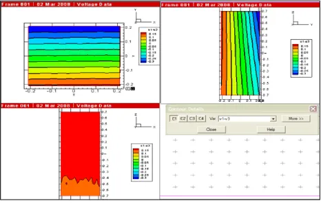
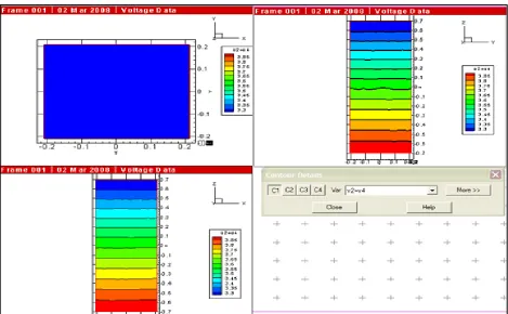
analyzed using TechPlot (Figure 36 - Figure 39).
41
Figure 37: HES2 (radial) output variation with respect to X, Y and Z co-ordinates.
42
Figure 39: HES4 (radial) output variation with respect to X, Y and Z co-ordinates.
Estimating the values of x, y and z (displacement along the X, Y and Z coordinates respectively)
from the outputs of the four sensors was challenging as it involved estimating three unknown
parameters with four boundary conditions. After much iteration, the best estimate of HES output
voltage as a function of coordinates (X, Y, and Z) was achieved with the maximum error of
1.5%. However, the estimated values of x, y, and z were far off the experimental values.
The combinations of two similar kinds of sensors, placed opposite to each other were analyzed
using Techplot. The 3-D plots analyzing the effects of these combinations; V1+V3, V1-V3,
43
[image:54.612.74.540.72.367.2]Figure 40: Variation of (V1-V3) in X, Y, and Z co-ordinates.
44
[image:55.612.73.542.383.673.2]Figure 42: Variation of (V2-V4) in X, Y, and Z co-ordinates.
45 Above plots were analyzed with the best estimate for the ‘Z’ axis derived by adding the outputs
from HES2 and HES4 (radial sensors opposite to each other). The voltage variation, i.e., V2+V4
with respect to Z axis were prominent in both XZ and YZ plane while almost negligible in the
XY plane. A solver tool in Microsoft Excel 2007 was used to derive the coefficients of the
equation:
z = -2127 (V2 + V4) + 7625 …Eq.15
where, z : Z co-ordinate (µm)
V2: Output voltage of HES 2 (V)
V4: Output voltage of HES 4 (V)
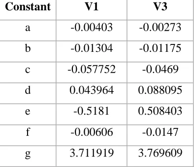
The voltage outputs for all sensors were estimated as a function of X, Y and Z co-ordinates. For
the axial sensors, the voltage equation was derived as the fourth order function of Z (axial
direction) co-ordinate and is:
V = a z4 + b z3 + c z2 + d z + e y + f x + g …Eq.16
where, V: Output voltage (V)
x: X co-ordinate (mm)
y: Y co-ordinate (mm)
z: Z co-ordinate (mm)
[image:56.612.208.405.507.676.2]a, b, c, d, e, f, g are constants listed in Table 3
Table 3: Constants for the estimation of voltage output for HES 1 and HES 3.
Constant V1 V3
a -0.00403 -0.00273
b -0.01304 -0.01175
c -0.057752 -0.0469
d 0.043964 0.088095
e -0.5181 0.508403
f -0.00606 -0.0147
![Figure 1: Implanted LVAD demonstration [3].](https://thumb-us.123doks.com/thumbv2/123dok_us/58091.5386/12.612.201.487.281.516/figure-implanted-lvad-demonstration.webp)