Superconvergence of numerical solutions to second kind integral equations

(1)

SUPERCONVERGENCE OF NUMERICAL SOLUTIONS

TO

SECOND KIND INTEGRAL EQUATIONS

by

G

.

A. Chandler

A thesis submitted to the Australian National University for the degree of Doctor of Philosophy

(2)

PREFACE

This thesis has benefited greatly from discussion with others. The existence of the singularities in the solutions of weakly singular equations was explained to me by Ivan Graham, and I thank him for the references [30] and [34] . The use of the adaptive method in chapter 5 for

pt-

00 _{was suggested by Mark Lukas.} _{My attention was drawn to} the duality argument of the finite element literature by Mike Osborne.

Otherwise, the results of the thesis are my

(3)

(ii)

ACKNOWLEDGEMENTS

The majority of the research for this thesis was undertaken in the

disgraceful circumstances created by the Australian National University's dismemberment of the research activity of the former Computer Centre. It is a considerable tribute to the quality of the staff and students of the resulting Computing Research Group that a suitable academic environment was created under such duress. I wish also to thank the Department of Pure Mathematics and the heads of the department (Professor N.S. Trudinger and Dr N.F. Smythe) for providing such suitable resettlement.

I wish to express my very great debt to my supervisor, Bob Anderssen. His enthusiasm for such a broad range of computational applied mathematics has been invaluable. His concern with, and attention to, the needs of his

students has resulted in supervision of an extremely high order. I am deeply grateful for all that he has done for me.

I acknowledge also the very close contact I have had with two fellow students; Ivan Graham from the University of New South Wales and Mark Lukas from A.N.U. In particular Ivan has generously expounded his unpublished ideas on the subject matter of chapters 4 and 5.

Many people had volunteered to help with the proof-reading; but only a few could be chosen. I thank Max Cohen , who utilized what she intended to be a purely social weekend, and Carolyn Lukas and Jacki Hickman.

(4)

ABSTRACT

This thesis examines certain numerical methods for the solution of second kind Fredholm integral equations of the form

( 1) X E [0,1]

where K is the operator defined by

--

fo

1

(Ku) (x) k(x,~)u(~)d~

Let u be the Galerkin solution to (1) using an n-dimensional space n

of piecewise polynomials of degree r as the basis space . It is known that //u -uo/1

~

O(n-r-1)

n oo Chapter 2 shows that if u _n is used to calculate the iterated Galerkin solution, u

*

=

f

+

Ku then (under suitable regularity

n n

conditions on k and f) the order of convergence is doubled to That is , u

*

is globall y superconvergent.

n If k

fails to satisfy the regularity conditions because of a discontinuity along the diagonal _X

₌

_~

_'

then u

*

n still exhibits this

- 2r-2

O(n )

super-convergence at the grid points, but not globally. Chapter 3 shows for smooth k and f that global superconvergence is preserved when the integrations required to form the Galerkin equations are performed numerically. The proofs of chapters 2 and 3 use the duality argument from the finite element

literature .

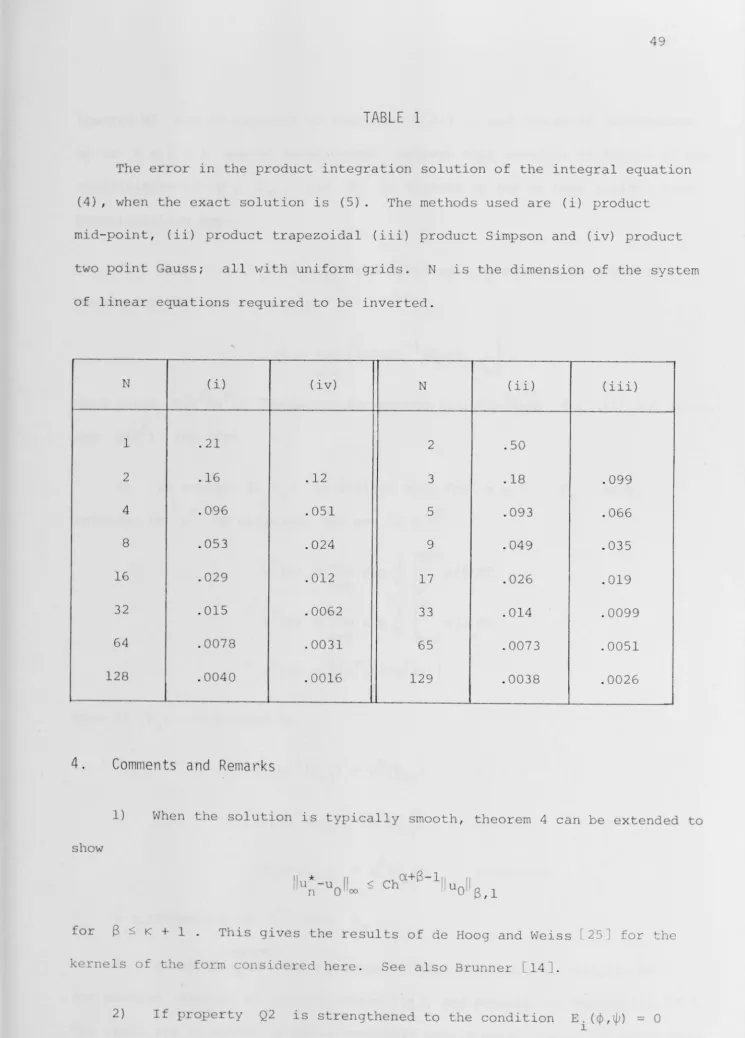
In practice the kernel function k is rarely smooth. Chapters 4 and 5 consider product integration solutions to (1) when the kernel is of

convolution type with a weak singularity. The high rates of convergence observed for the product integration solution when u

0 is smooth have been explained previously. However the singularity in the kernel introduces certain typical singularities into u

(5)

(iv)

Chapter 4 uses a modified duality argument and a characterization of the

singularity of the solution in terms of Nikol 'skii s9aces to prove these reduced orders of convergence.

Chapter 5 reports numerical experiments which indicate that the order

of convergence can be restored 'by using an appropriate non-uniform grid.

Such grids may be generated automatically by an adaptive method. This method uses the characterisation of the product integration solution as an

(6)

PREFACE

ACKNOWLEDGEMENTS ABSTRACT

INDEX OF NOTATIONS

CHAPTER 1: PROLOGUE

INDEX

OF

NOTATIONS

This index lists some notations which are used throughout the thesis. It does not include some of the temporary notation used from time to time.

Operators

I

K

p n

'

p

n

F

u

nc

t

i

ons

u

n

*

u n

( k) u

The identity operator.

See equation (1.1) .

A projection operator. See p . l for its use in chapter l , p .19 for its use 1n chapters 2 and 3, and p .43 for its use 1n chapter 4 .

p

=

I - p

n n

The kernel function, solution and right hand side of the integral equation (1.2) .

The projection solution (p.l, p . 20); but see also p.50 for its use in section 5. 3.

The iterated projection solution (p.2, p.20), and 1n chapter the product integration solution (p.47).

(9)

Function

Spaces

and Norms

II

• II

L p (St)

' ll· llp,s-2

ck (St) _, ₁₁_• ₁₁

,k,oo,[2

CCL (St)

' ll· IICL,oo,s-2

*

wk (St)

' II· llw,k,p,s-2 p

CL

N l (St) _' _II _·_IICL_,1,_s-2

\) Sp6

(C

,JP r)

s

n

Miscellaneous

C

Uf;2

In chapter 1 denotes II • 11 . 00

p .8.

p .70.

p .

7

0 ,

p .18.

P.19.

p .8.

The generic constant, p.9, p.19.

The difference operator, p .18.

{xEs-2:x+sESt} , p .8.

A quadrature rule p .34 .

(viii)

Theorem c .n denotes theorem number n of chapter c , theorem n

denotes theorem number n of the current chapter. Similarly with equation

(10)

CHAPTER 1 PROLOGUE

1. Introduction

This thesis analyses certain methods for the numerical solution of linear Fredholm integral equations of the second kind on a finite interval. We suppose that we are given an integral operator K defined by

(1) (Ku) (x) =

1

k (x,~)u(~)d~ • X E I= [O,l] •

I

and we wish to approximate the unique function u

0 satisfying the equation

( 2 ) (I-K)u

0

=

f

where f is a known function and I denotes the identity operator. For the subsequent mathematical analysis we wish to regard (2) as an operator

(X)

equation on L Hence various conditions are placed on · k to ensure that

(X)

K is a compact operator on L But we assume without further explicit

(X) (X)

mention that (2) is

well posed

on L that is for every f EL there

(X)

exists a unique u

0 EL such that (2) holds.

(X)

Let S be an n dimensional subspace of L (the

basis

space

)

and n

(X)

let P be a projection of L

n onto S n

(2) is a function U E S

n n satisfying

( 3 ) (I-P K)u = P f

n n n

Then a

projection

solution

to

Such approximate solutions have been extensively studied, and their existence,

uniqueness,and rates of convergence are well understood (Krasnosel'skii

et al. [28] , Ikebe [26] and the references given there) . However, following

the suggestion of Sloan et al.

(

[3

7 ]

,

[

37 ] [39] [

41 ]

and [42]) , let us apply

the

natural iteration

,

u ~ f +Ku, to u

(11)

2

u is viewed as an intermediate step in the final calculation of the

n

iterated

p

rojection

solution

( 4) u

*

=

f + Ku

n n

Although u*

n has been observed to have a higher rate of convergence than u this is not well reflected in the existing error estimates.

n

It is clear that the natural iteration will not damage the order of

convergence obtained; for

( 5) u* - u

n 0

shows

for some constant depending only on K . Further, using (5) and the

compactness of K , Sloan [38] has shown under fairly general conditions that

( 6) _jj_u*_-_u

II

n 0

Hence the order of convergence of u*

n is greater than that of u n

But i t is well known that (6) is by no means an optimal estimate. It

is easy to see that

( 7 )

u*

n satisfies the equation

( I -KP ) u

*

=

f . n n

Under mild conditions on K and P i t can be shown that KP is a

n n

00

sequence of consistent (K u~Ku for all UEL ) , collectively compact operators n

approximating K. Thus i t follows (Anselone [ 2 ] , Atkinson [ 3 ] )

is uniquely defined by (7) and

(12)

( 8)

for some constant C depending only on K.

Now consider the particular example in which

s

lS the set of

n

piecewise polynomials of degree r on a uniform grid and p lS the

n

interpolatory projection defined so that p u interpolates u at the r + l

n

Gauss-Legendre points on each subinterval . Then u is the collocation

n

solution to (2) and u*

n is the product integration solution. It is known

that while i t follows from the results of de Hoag and

Weiss [25] applied to (8) that _llu*-u

JI

n 0

assume that k and are smooth. )

-2r-2

=

O (n ) . (Both these estimates

Thus the order of convergence of

u* is twice that of u

n n showing that the error bound (6) may be

significantly improved in certain situations.

The higher rate of convergence of u*

n is to some extent surprising.

The O(n -r-1 ) convergence of is optimal in the sense that

is also O(n - r - 1 ) Thus i t is unexpected that

u

n could

be used to generate such a higher order solution. Such faster than optimal

convergence is called

superconver

gence

.

Besides product integration, the best known projection method is the

Galerkin method. Given an appropriate

s

n p n is chosen to be the

orthogonal projection in the L2 sense ("least squares" projection). In

this case there are no existing superconvergence results analogous to those

for product int gration. This obvious gap is filled in chapter 2. When

piecewise polynomials (i.e . splines) of degree r are used as basis functions

i t is shown that

ll

u~-u

-2r-2

0

JI

=

O(n ) when the

kernel and the solution have r+lth derivatives. Moreover, if the kernel

(13)

4

diagonal x

=

~ (for example Green 's functions of ordinary differential equations) , then u* will be superconvergent at the knot points, but not

n

globally. The basic step in the proof of these results is the application of the Aubin-Nitsche duality argument of the finite element literature

(Strang and Fix [ 43]) .

An essential limitation on Galerkin methods is the necessity to perform the required inner products analytically. In all but the simplest cases this is impossible , and quadrature must be used. The solutions obtained in this

fashion will be called the discrete Galerkin solution and the discrete

iterated Galerkin solution. Chapter 3 gives an error analysis of these two

methods. The main result is that if f and k have 2r+2th

derivatives and if composite quadrature rules of sufficiently high degree

are used, then the discrete iterated Galerkin method has the same

super-convergent behaviour as the (exact) iterated Galerkin method. Such results

are common in the numerical solution of differential equations , but are rare for integral equations.

When discontinuous splines are used the discrete iterated Galerkin method reduces to a Nystrom method, and the results of chapter 3 give the expected orders of convergence under much the same conditions as the standard analysis

(Atkinson [ 3 ]) . However when splines of high continuity are used, the

discrete iterated Galerkin methods are a new class of methods whose convergence has not previously been examined.

Although integral equations with smooth kernels occur in p4actice, they do so infrequently. Thus the final two chapters of the thesis consider product

(14)

is that the singularity in the kernel prevents the iterated solution

achieving the full order of superconvergence. Thus, for example, when the

kernel is

(9)

the order of convergence of the collocation solution, O(n -r-1 ) , increases

by only O (n -~)

3

to O ( n - r-

12 )

_{for product integration} _(i.e. _iterated

collocation); rather than to O(n -2r-2 ) when the kernel is smooth (de Hoag

and Weiss t25]) . The second and more serious difficulty is that the

singularity of the kernel introduces singularities into the solution at the

endpoints. Thus even if f is smooth, the solution to (2) with kernel (9)

will be of the form

+ "smoother terms"

where and b

0 will in general be nonzero (Richter [34]) . This has

serious consequences for numerical solutions . The order of convergence of

_1.,

the collocation solution on a uniform grid is now O(n 2)

The product integration solution increases this to O(n-1)

has not been proved in existing results.

which is optimal.

however this

In chapter 4 the observed rate of convergence for product integration

is proved. It follows from the results in chapter 4 that if

( 10)

where m is smooth and o(x- ~)

=

lx-~ja-l (O<a<l) then the product

· · · h O (n-2a)

(15)

6

The prerequisite for proving the results in chapter 4 is an adequate characterization of the smoothness of the solution. This is provided in section 2 of chapter 1. We prove there general results which show that for

the kernel (10) belongs to a particular Nikol'skii space This

means simply that the derivative of the solution satisfies a certain generalized Holder continuity condition. (The appendix gives a self contained exposition of the results we need about Nikol 'skii spaces.)

The main step taken in chapter 4 is a modification of the duality

argument to make i t applicable to product integration. This is essentially an abstraction of the classical proof of the convergence of composite

Gaussian quadrature formulae . The required convergence result for product

integration methods follows by using an approximation theoretic property of l+a.

N

1 in the duality argument to produce the bounds required by the theory of collectively compact operators.

From a practical perspective these results are not encouraging. The convergence for the kernel function (9) is only modest. The final chapter of the thesis, chapter 5, reports some successful numerical

experimentation with ways of increasing the order of convergence by using an appropriate non-uniform mesh.

We consider the second kind equation with kernel (9) and solution

~ ~

=

X

+ (

1-x)

(which has the typical singularities expected of the solution) . Use of product integration with the mesh points "clustered" around the end points

increases the order of convergence to that expected when the solution is 31..

O(n- ")

(16)

set of experiments is with an adaptive method of generating such meshes.

This makes essential use of the fact that product integration is iterated

collocation (for a general kernel (10) with m11 the iteration is not

precisely the natural iteration, but the extension to cover this case is

minor) . Because (5) shows that the error of product integration depends

only on the error of the intermediate collocation solution, we hypothesise

that a grid giving an accurate collocation solution will also give an

accurate product integration solution. A grid for the collocation solution

is generated by successively refining those subintervals on which the

collocation solution has the largest error. But since the actual solution

is unknown the error must be estimated. This is done by comparing the

collocation solution with the more accurate product integration solution.

When the product integration solution is calculated from the collocation

solution on the adaptively generated grid, the order of convergence i s again

that expected with a smooth solution.

2 .

Smoothne

s

s of s

ol

ut

io

n

s

o

f se

cond kind equat

i

ons

The numerical methods discussed in this thesis are based on finding a

good spline approximation to the solution. The existence of such an

approximation cannot be guaranteed unless the solution is sufficiently smooth.

Since the solution is unknown such smoothness has to be deduced from the

behaviour of the right hand side and the kernel. Results of this type are

collected in this section for use in subsequent chapters . Theorems 1 and 2

are straight-forward theorems of this nature; and they are sufficient for

the needs of chapters 2 and 3. The remainder of the section proves the more

involved theorems needed in the study of weakly singular kernels of

convolution type in chapter 4.

(17)

8

example Gilbarg and Trudinger [21] ). Note that if the weak derivative is continuous then the function is continuously differentiable (more strictly,

equal a .e . to a continuously differentiable function) and the weak derivative coincides with the usual (strong) derivative.

For any non-trivial compact subinterval n C IR the LP(n) norm lS

written ll · llp,n ; or if n is understood we write LP and ll · llp .

(n may be similarly omitted from all other spaces and norms.) For any

· t k

o

Ck(n)

in eger ~ , H denotes the Banach space of functions with k

continuous derivatives under the norm

A number of times we use the fact that

II

· II

is equi· valent to the norm

C,k,co

(1) (k)

max{ llull , llu

11 ,

...

, lju

II}

.

co co co (CO will also be abbreviated to

C

.

)

For any non-negative real number a , we write a= [a] + a

0 , where

[a] is an integer and O < a

0 $ 1 . Then the space of a-Holder continuous

functions, Ca (n)

*

functions for which

where

and

is the set of all [a] continuously differentiable

l

u

l

_a_,_co

}

< co

(6. u) (x) = u(x+E:) - u(x)

E:

Again is equival ent to the norm max { II u II , 11 u ( 1) 11 , · · · , 11 u ([ a

J

)

I ,

I

u

I }

·

(18)

The spaces C k and

C

a

may be generalized to domains

St

c JR.n , n > 2

*

(Kufner et al. [29]). In this case

where

sup sup

s>O e.

l

( 6 . u) ( x)

=

u ( x +s e . ) - u ( x)

l,E l

and {e

1, .. ,en} is the canonical basis of JR.n

Throughout this thesis C denotes a generic constant, no two

occurrences of which are necessarily the same. In this section C depends on K and the order of the differences and derivatives involved. However C is independent of u

0 and f and any other functions appearing in the statement of the theorem.

For any function of two variables v(x,~) v (~) = v(x,~)

X

v denotes the function X

Since we are almost exclusively concerned with functions defined on the

unit interval we shall suppress I in writing norms and spaces. With the one specific exception mentioned below 11 • llp ,

Ck

etc . are to be understood

as

II II

_• _p _,_I and

Ck

(I) etc.

THEOREM

l:

Suppo

s

e

o

r

each

X E I .,

k

_E _L1

and

_ll

_k

_)l

_l

~ _C

_uniformly

X

wi

th

r

e

s

pe

ct t

o

X •

In

addition assume

f

o

r

some intege

r

Q,

~ 1

,

k

(i -1, 0) E L 1

_{and that}

_f

_or

_all

E > 0

_and

'

X E I E

f

Jk(l',-l,O) (x+E,i;) - k(l',-l,O) (x,i;) Jdi; <; CE

I

un1., ormly 1.,n

x .

Then

K

1.,s a bounded operator

L

00

~

CQ, (and therefore

(19)

10

00

compact on

L

J

• Hen

e

implies

Proof:

An application of Fubini' s theorem and the definition of weak

00

derivative shows that for any u E L Ku is (£-1)-differentiable and (Ku) (Q.-l) (x)

=

f

k (Q.-l,O) (x,I;) u(i;) di; . Further

shows with

Finally as u

0

=

f

+

Ku0 ,

00

because K is compact implies (I-K) has a bounded inverse on L

00

(Recall (I-K) is well posed on L) .

/Ill

We turn now to a more special class of kernels in which k has the form

( 11)

k(x,~)

=

k

1 (x,~)

=

k

2 (x,~) ~ ? X

and where for two integers £ and m

- 1 $ m $ £ 0 $ £

'

k E Cm(IXI) and

£

kl E C ({(x,~)EIXI:~$x})

(12)

£

k2 E C ({(x,~)EIXI :~?x})

(When m

₌

-1 k lS allowed to be discontinuous

'

at X

=

~)

.

Two obvious examples of such kernels are Green's functions for ordinary

(20)

THEOREM

2:

Suppose

k

has the form

(11)

with the

conditions

(12)

holding

.

Then

( i)

( ii)

( iii)

Hence if

Proof

:

Then

a bounded operator

1 -+ C

and

compact

1

K

i-s

L

on

L

CX)

cm

when

m ~ ₁ K

i-s a bounded operator

L -+

and

'

.,

for

p < ,Q, - 1

.,

K

i-s

.

a bounded

operator

cP-+ cp+1

f E c£

'

u0 E ci

.

The proof of (i) follows by writing

(Ku)

(x)

=

Ix

k

1 (x,()u(()d( +

Il

k2(x,()u(()d(

0 X

(K

1 u) (x+E) - (K1 u) (x)

=

J,x (k1(x+E,() - k1 (x,())u(()d(

0

+

l

x+E

k(x+E,~)u(~)d~

X

I

x+E:

~ csl!ull₁ + c

lu

(

~

)

la~

.

X

Thus

I

(K

1u) (x+E) - (K1u) (x) I-+ 0 as E:-+ 0 . Hence K1u is continuous,

and an elementary argument shows l!K

1 u1!00 < c l!ull 1 . A similar argument shows

K

2 and hence K is bounded L 1

-+

C.

Further as

(1)

rox

(1,0) Jl (1,0)

(Ku) (x)

=

Ji

k

1 (x,~)u(~)d~ + k2 (x,~)u(~)d~

X

we have that Ku E

w

1

1 and

+ ~

1 (x,x) - k2 (x,x)Ju(x)

(21)

12

embedded in L1 (an immediate corollary of theorem A.7) part (i) follows.

Part (ii) is standard.

If u E Cp then

(

0

x

(1

(Ku) (p+l) (x)

~

J,

kip+l,O) (x,i:;)u(i:;)di:;

+

J

k~p+l,O) (x,i:;)u(i:;)di:;

X

where

Thus part (iii) follows.

Finally as

uo = f + Ku₀ =

we deduce u

0 E ci and

llu(.Q,) 11 ~ 0 00

+

p

l

(b.u)p-i(x)

l

i=m+l

k (i,0) ( )

2 x,x

i-m

(I+K+ . . . +K )f + K .Q,-m+ 1 u 0

c llf /1.Q, ,oo + c lluo/100 < Cl/f _{/1.Q, 00}

'

(as (I-K) has a bounded inverse).

_Ill/

The remainder of this section studies operators of convolution type.

That is we suppose the kernel function k is of the form

( 13) _where

Al : for some a , with O < a ~ 1 , o E Na

1 and

A2: m E C 2 (

rxr)

.

(Since O is required to be defined on [ -1,1] we take the expressions a

o E N

1 to refer to [ -1,1] as the domain.) A typical example

(22)

sufficient to ensure that K is compact L ~

C

(see Zabreyko et al. [47]

p .91 and Graham and Sloan [23]) .

Finally, before proving the main regularity result, theorem 6 , and its

preceding lemmas, i t is convenient to introduce the operator L defined by

(Lu) (x) -

J

O(x-~)u(~)d~ .

- I

Notice that K may be alternatively defined by

LEMMA

3:

Proof

:

(Ku) (x)

=

(2:: (m u)) (x) .

X

Under assumption Al is a bounded operator

For any

s

> 0 and x E

Is

( 6 o) ( x-~) u ( ~) d~ ,

s

and hence by Young's inequality

Thus

Another application of Young' s inequality gives

and hence

1

L

as required. ////

LEMMA

4:

Under assumptions Al and A2 K is bounded.

(23)

s(x)

=

fx

CT(~)d~ .

0 1

Then for any u E

w

1

(Ku) (x)

=

{L{mu)){x) X

=

-s(x-~)m (~)u(~)

~=l

~=O X

+

f

I

( 1)

s (x-~) (m u) (~) d~ . X

Thus Ku is weakly differentiable with

Further

shows

(14)

( 1)

(Ku) (x)

=

- O(x-~)m (~)u(~) X

~=l

~=O

~-1

( 1, 0)

- s(x-~)m (~)u(~)

x ~=0

f

s(x-~)m(l,l) (~)u(~)d~

I X

~=l

f

~=O I

+

f

I

o (x-~)u(~)m(l,O) (~)d~ X

(Ku) ( l) (x)

=

~=l

O(x-~)u(~)m (~) X

~=O

+ (Z::(m u(l)) (x) + (Z::(m(l,O)u)) (x)

X X

14

Now to prove K is bounded it is required to show that for each of the terms, _T. _'

(24)

11

6

T.

II

S 1 l,I

s

But for the first term this follows by using theorem A.4 and Leibnitz's

formula for differences to show

The second term is bounded by observing

(15)

+

I(

L ( ( m -m ) u ( 1) ) ) (

x)J

.

L

x+s x

Now applying lenuna 3 to the first terms of (6) (that m of lenuna 3 has

X

been replaced by x + s is irrelevant here), leaves only the second terms. But then an application of Fubini's theorem shows

JO

(

x-~)

J J

m ( ~) -m ( ~)

J

ax]

J

u ( l) ( ~)

I

d~

x+S X

which gives the required estimate. The third and fourth terms of (5) are bounded similarly.

THEOREM 5:

Under

• a

s

umption

Al

and

A2.,

l+a.

on

N

1 .

Proo

:

From theorem A.7

Therefore, as lenuna 4 shows compact.

the inclusion l+a.

1

K ~s

a compact ope

r

ator

is compact. is bounded, is also

(25)

16

The assumption that m E C 2 ( IXI) can be slightly relaxed. It suffices to assume that there is a bounded subset of containing, for any

~ . (1,0)( )

choice of x and s , the functions m x,• m (0,1) ( X, • )

m(l,O) (•

,

F;,

)

and m(O,l) (•,F;,). The above proofs carry through with only

minor modifications.

THEOREM

6 :

Suppose

K

satisfies

Al

and

A2.

and

Then

f

E N1 +ex

1

implies

1 +ex

u₀ E Nl

Proof

:

If 1 is not an eigenvalue of K considered as an operator on

C

i t is not an eigenvalue of K considered as an operator on N 1 +ex (because

1 1 +ex

Nl

CC)

.

Therefore by theorem 5 and the Fredholm alternative, there is a unique such that (I-K)u

0

=

f and

1 +ex

if f E Nl

II u O 11₁+ex , ₁

~

c

11 f 11₁+ex , ₁ and

C

must coincide.

Again since _Nl1 +ex

_CC

_'

the solutions in

Ill/

Consider application of theorem 6 to the particular kernel function (9). Assumptions Al and A2 are satisfied with ex=

12 .

Thus by theorem 6,

3

for f sufficiently smooth, u

0 E

N{

2

• But this is precisely the result

expected from the expansion for _uo obtained from Richter [34] ; for the function _X1/2 E N 3/2 but 1/2 _~ NB when B > 3/2 _{Thus theorem} ₆ _{is the}

1 ' X 1

.

best possible result in the sense that no matter how smooth f 1 +ex

'

u0 E Nl

but B> l + e x .

3. Notes and Remarks

1) The introduction of the natural iteration for general projection

methods is due to Sloan. However i t had been previously used implicitly in

the product integration method, and is similar to the natural interpolation

(26)

2) The methods of theorems 4-6 can be modified to prove more general results when the integral equation is not well posed . Following theorem 4, i t can be proved under Al and A2 that for

B

~ 1 , U E implies

2

116

Kui!₁ I

€ ' 2E

< a+BI I

CE u B, l .

Then provided a+B ~ 1 , the reiteration theorem (Butzer and Berens

l

161

p .259, and making suitable modifications to the unit interval I , instead of IR) shows Ku E _Nla+B

.

Hence when a lS irrational , we have the chain

implications, Ll ~ Ku a =} 2 2a m ma

of u E E _Nl K u E _Nl I • • • K u E _Nl I where m

lS the smallest integer with ma > 1 ( If the a of Al lS rational,

choose a ' irrational s . t . ma > 1 implies ma' > 1 and use the above a ' instead of

.

) Thus ma 1 we have

argument on a as _Nl C

w

1 I

(m+l) (l+a)

if (I-K)u

=

l+a implies l+a

K u

0 E Nl Thus f I f E Nl uo E Nl

0

whether or not _uo lS a unique solution of the integral equation. For

example, this argument shows the eigenvalues of K belong to The reiteration theorem however is not elementary.

3) The regularity of the solutions of convolution type integral

equations have also been studied in Richter [34] , MacCamy [30], Schneider [ 36]

and Graham [22] . See also the discussion of Mayers [32] and Baker [6].

4) A comparison of the convergence of projection, iterated projection

and other classes of methods for eigenvalue problems in an abstract setting

is contained in Chatelin (18] and the references given there. However explicit

orders of convergence are not derived. The natural iteration is discussed from

more general perspectives in the reviews of Noble [ 33] and Sloan [40] . A

sununary of various superconvergence phenomena for collocation solutions to

various classes of integral and integro-differential equations is contained

(27)

18

CHAPTER 2 GALERKIN METHODS

1. Introduction

In addition to the assumption that the second kind integral equation is

well-posed, we assume that

Hl: for all X E I ,

JJk)i 1 ::; C and

k

X

1

E L

co

and uniformly with respect to _{X '}

Hypothesis Hl ensures that K L ~

C

is compact (Zabreyko [47 ] , Graham and Sloan [ 23]) , but still admits a large class of kernels. In order to prove the superconvergence results of this chapter much stronger conditions

must be imposed . Thus we will further assume

H2 : there exists a positive integer £ such that for each

X E I , kx E w£

1 and JJk)lw,£,l is bounded uniformly with

respect to x .

Let 6 be a partition, 0

=

x

0 < x1 < ... < xn

=

1 , of t he uni t interval. Let I. = [x.

1,x.

J

and h. = x .

-

x . 1

.

Let h = max (h. ) and

l i - l l l i - l

let a = max (h.) / min (h.) . For any integers r and \) such that r > 0

n l l

and -1 $ \) $ r let S_p6

(C

\) _,JP_r) denote the set of functions ¢ such t hat

( i)

( ii)

for each _l _' E JP r

degree ::; r) and

if v ~ 0 then

_¢

_E

_C

\)

_.

(where JP

(28)

If V

=

-1 then a function is possibly discontinuous at X. l

and difficulties arise in the definition of ¢(x.)

l Any sensible convention

will do, but for definiteness it is assumed that ¢ is continuous from the right and continuous from the left at 1 .

The set Sp6

(C

\) ,JP r) will be called the

continuity

v

.

For simplicity we shall write

splines of degree

s

n for

r

and

when no

confusion can occur. The points x.

l will be cal led

knot points

.

Throughout

chapters 2 and 3 P denotes the orthogonal projection of L2 onto S

n n

Finally we assume in this chapter and the next that the partitions 6

are quasi-uniform: that is for some value of

o

~ 1 which remains fixed,

o

~

o

for all partitions 6

n The generic constant C introduced in

chapter 1 is now allowed to depend on r , V., and

o

,

but is otherwise independent of the partition.

The required approximation theoretic properties of

the following lemma.

LEMMA 1

:

( i) For all

( ii) For all

r+l

U E Wl

U E cr+l

*

II u-¢ 11₀₀ <

there exists ¢ E S

n

r+l,l

there exists _¢ _E

s

n

r+1

I I

Ch u r+l,oo

( iii) For 1 ~ p ~ CX) p _lS a bounded map

LP

n

where C lS independent of p and 6

.

s

n are stated in

such that

+

LP

_with _!I_{P n}

_II

< C,

Proo

:

Parts (i) and (ii) follow from de Boor and Fix [10] , part (iii) from

(29)

Since P' (P' denotes (I-P )) is bounded on LP , and since

n n n

P' cp

=

0

n for any cp E S n

1/P 'ul/

=

1/P' (u-cp) II $ IIP' II llu-¢11 ·

n p n n p

Thus the estimates in (i) and (ii) hold for cp

=

p u n

2. Global

Superconvergence

20

The

Galerkin

solution

to the second kind equation (1.2) is defined by

( 1) U E S

n n

The proof of the convergence of which are required in section 3.

u

n

(I-P K) u

=

P f

n n n

is well known; and we state results

THEOREM

2 :

Suppose

Hl

holds and

u

0 E c:+l

Then for

h

sufficiently

small

the

Galerkin solution

is uniquely defined

by

(1)

and

r+1

I I

llu _n-uoll _oo :s; Ch uO _r+1 _,_oo .

Proof

:

The proof follows from Krasnosel'skii et al.[28] p.210 and their

lemma 15.4 p .212; using lemma 1 to verify the appropriate conditions. ////

Recall from the introduction that the

iterated

Galerkin

solution~

is defined by

( 2)

It may be readily verified that

( 3)

u*

=

f

+

Ku

n n

u* satisfies

n

( I -KP ) u *

=

f .

n n

The following lemma shows that (2) and (3) are equivalent definitions of u*

n '

(30)

3 :

Equation (1) has a unique solution for every f iff (3)

has a unique solution for every f .

Proof

:

If u is a solution of (1) then f

+

Ku is a solution of (3)

n n

and if u* is a solution of (3) then Pu* is a solution of (1). Thus (1)

n n n

has a solution for every f if and only if (3) does. But I - p K lS a n

linear operator on the finite dimensional space

_s

_'

n and (3) is equivalent to the linear equation

( I -KP ) v

=

KP f n n n '

on the finite dimensional space KS n

U

=

f + V

n n '

Thus for both (1) and (3) the

condition that there exists a solution for every value of the right hand side is equivalent to the condition that there exists a unique solution for every

value of the right hand side.

_Ill/

Given the equivalence of (2) and (3) , either equation may be used as the basis of an error analysis . In this section we use (3).

THEOREM 4

:

Asswne

Hl

and that

H2

holds for some

positive

i

,

V < £ ~ r

+

1 .

Then

for

h

sufficiently small

u*

is

uniquely

n

defined by

(

3).,

_{and if}

_u

_C

r+l

0 E

*

then

00 00

Proof

:

The operators KP '

n L -+- L converge in norm.

00

u E L

For if

(4) ( KP I u) ( X)

=

(

k , p I u)

= (

p I k p I u )

= (

p I k , u)

n x n n x' n n x

and thus by lemma 1 and H2 ,

(31)

22

Hence it is standard to show from (3) that

But again by (4) and lemma 1 ,

II KP I uo 11 ~ C II p I k 111 II p I u O II

n

00

n

x

n

_oo

r+1+i 1

I

~ Ch

u

₀ l .

r+ ,oo

/Ill

The crucial step in theorem 4 is (4). This is the Aubin-Nitsche duality

argument from the finite element literature.

C

r+l .

To apply theorem 4 i t is necessary to verify the hypothesis u

0 E

*

This is most easily done if for some constant C independent of x ,

(5)

(

I

k ( r ' O) ( x+E , ~) - k ( r 'O) ( x, ~)

I

d~

~

CE

JI

Theorem 1.1 then shows _u

C

r+l .

0 E * Thus we have the following theorem:

THEOREM 5:

A

ss

ume

Hl ., (5) .,

and

t

hat

H2

holds

f

o

r

Q,

=

r

+

1

Then

J

l

u*-u

II

< Ch 2r+2 J f

I

.

n

O

00 r+l,00

/Ill

Alternatively the smoothness of u

0 may be inferred if k has the special structure (1.11) . Thus suppose k i s the Green's function defined by

k(x, E)

=

(e~-1) (ex-l_l) (1-e- 1)e~

( 6)

(32)

C

r+l cr+l . Then theorem 1.2 shows that f E * implies u

0 E * Whence as

kx E W~ , a direct application of theorem 4 with £

=

1 shows

ll

u*-u

II

~

Chr+2 If I

n O 00 _r+l,00 _'

provided the continuity of the splines is selected so that V

=

-1 or V

=

0 . In fact more is true. A direct argument shows there exists

V

¢

E sp

6 (C

,IPr) for V

=

- 1 , or V

=

0 and r ~ 1 , such that

2

< Ch .

Use of this estimate in the proof of theorem 4 shows

( 7) 1/u*-u

II

~

Chr+3 lfl

1 . n O 00 r+ _,_oo

3. Local Superconvergence

Section 2 gave an order of convergence result for the. iterated Galerkin method using equation (3). This section uses equations (1) and (2) instead, and makes estimates directly from the relation (see equation (1.5))

u*-u n 0

This analysis yields better error bounds for the iterated Galerkin solution at the knot points when the kernel has the discontinuities typified by (6).

1ve assume (as in (1.11) and (1.12)) t hat

( 8)

(33)

24

-1 $ m $ !l

'

0 $ !l

'

k E Cm(IXI)

'

Q,

E;, x})

( 9) _kl _E

C ({

(x,E;,) E I X I $ _and

Q,

E;, x})

k

2 E C ({(x,E;,) E I X I ~

Define the adjoint operator K* by

-- J,l

K*u(x) k(f;,,x)u(E;,)df;, .

0

LEMMA 6:

I - K* is well posed on L 00

Proof

:

Under the conditions (9) K maps L1

~

C and K is compact on L1

00

and L

posed on

00

u E L

(theorem 1. 2) . Hence, as K

1

L (If u E L 1 satisfied

00

is well-posed on L K is well

(I-K)u

=

0 , u

=

Ku implies and thus u

=

0). Therefore, as the integral operator K* is also the Banach space adjoint operator of K on (L1)*

=

L00 the Fredholm alternative (Yosida [46]) shows that K* is well posed on L 00

_/Ill

Lemma 6 shows that for each x E I there exists a unique function g E L

X

00

such that

(I-K*)g

=

k

X X

The structure of is given in the following lemma.

used to denote the function

E;,l

=

E;,l

+

=

0 E;, < 0 .

The notation E;,l

+ lS

LEMMA 7:

Let k be a kernel of the form (8) with conditions (9) holding.

Then for each x EI _there _{exist constants} _am+l(x)_,_..._,a_Q,(_x)

function

¢

defined by

X

(34)

<P (~)

=

X

has the properties

(10) Q,

l

i=m+l and l

a.(x)(~-x)

l

+

for some constant C independent of x .

Proo

f:

Let

µ

= max{m,O} . Then

g

=

k + K*g

X X X

Q-1µ = (I+K*+ ... +(K*) " )k

X

As theorem 1.2 shows (K*)Q,-1µ+lg

X

Q,

E C ,

+ (K*) Q,-1µ+lg X

II (g - (I+K*+ ... + (K*) Q,-1µ) k ) (Q,) II

~

c llgxlloo < C

X X oo

(by lemma 6 and the Fredholm alternative, I - K* has a bounded inverse on

00

L and Ilg II

~

ll (I-K*)-111 Ilk II

~

C).

X oo X oo Since k X and K* are known, there

is now no difficulty in principle in writing down the form of the

discontinuities in (i.e. of (I+K*+ ... +(K*)

t-w

)k ) . X

manipulations are outlined briefly.

( 11)

where

Define \l' by

X

Q,

\l' (~) =

X

l

i=m+l

l

b. (x) (~-x)

l +

b. (x) = .1, (k

2(0,i) (x,x)

l l .

Then k - \l' E CQ, and theorem 1.2 shows

X X

(12) g - (I+K*+ ... +(K*) Q,-1µ)\l' E C Q, •

X X

Now define an operator R by

( 13) ( Ru) ( ~) ₌

J

_\l' ₍_~_)u _(T) _d_T _.

I T

(35)

26

Then as k

T

Q,

\PT EC ' (K*-R) is a bounded map

00 Q,

L -+

C

.

Thus writing

K* = (K*-R) + Rq J.n ( 12) and using theorem 1. 2 to neglect terms of the form

shows

(14) g - (I+R+ ... +R

£-µ

)\¥ EC !l .

X X

Now lemma 8 below shows that for any i < £

Q, .

l

R((•-x)) -

l

c .. (x)(•-x)J E C Q, •

+

. . 2 lJ +

J=m+i+

Thus by the definition of \¥

X in ( 11)

i=2m+3

dl. (x) (~-x) l E

C,Q,

l +

where

i-m-2

dli (x) =

I

j=m+l

c .. (x)b.(x)

Jl J

Using RP= R(Rp-l) and proceeding inductively gives

( 15)

where

Q,

l

i= (p+l)(m+l)-1

i-m-2

l

d .(x)( •-x)

pl +

d . ( x)

=

l

c .. ( x) d

1. ( x)

pi i=p(m+l)-1 Jl p- J

The required expression for

cp

X is obtained by substituting (15) in

(14) and collecting terms. The bound (10) follows from an inspection of the

terms in which were successively neglected in the above proof.

/Ill

To complete the proof of lemma 7 we prove the promised lemma.

LEMMA

8:

Let R be defined by (13) and (11), and suppose the conditions of

lemma 7 hold. Then for all i , 0 ~ i ~ Q, , there exist constants

c. .

2 ( x) , ... c. 0 ( x) such that

(36)

Proof

:

Q,

l

R( (•-x) ) -

l

+

_j=m+i+2 C , . lJ (x) (•-x)+J E CQ, •

A direct computation shows

Q,

l

j=m+l

9,,-i-l

=

l

j=m+l

b. (T) (t,;-T) J (T-x) 1dT

J

.

I J

+

c- i+j+l

( s-x)

+

J

b.(x+(E,:-x)T) (1-T)JT

1

dT

I J

Since b. E

C

£

-i

, the Taylor expansion of b.

l about x shows that the

l

function

J

I b. (x+(E,:-x)T) J (1-T) JT1dT

!l-(i+j+l) b~k)

l

(E,:-x)k _J~

k=O k !

(1 . . k

J

(1-T)JTl+ dT

0

lS at

t,;

=

X . Thus collecting powers of (E,:-x)+

gives lemma 8 with

C . . ( X)

=

l ]

j-i-m-2 b(k)

I

j-i-k-1

k!

k=O

j-i-k-1 i+k

( 1-T) T dT

If the point x of lemma 7 happens to be a knot point X. I l

Thus applying lemma 1 to shows that

IIP'g 11

1

~

Ch!l+l . This is not true for an arbitrary point x .

n xi

then

i n ( 16)

Ill/

Given the structure of the proof of the local superconvergence

result follows by the duality argument and theorem 2 .

THEOREM 9:

Suppo

s

e the ke

r

nel

k ~

o the

f

orm

(8)

with condition

s

(9)

hold

i

ng

o

r

v

s

m

s i s

r

+

1

po

int

x . .,

l

(37)

where the constant

Proof

:

Since

I

u * ( X. ) - uo ( X. )

I

n l i

C bS

independent

of

X. • l

=

K (u -u

0) (x.)

n ~ = (k X, ,u -uo) n l

=

(g , (I-K) (u -u

0))

xi n

lu*(x.) - u (x.)

I

n l O l = !(P'g n x. ,Pn '(I-K)(u n -u0))! l

28

Theorem 9 now follows from theorem 2 and the remarks given after

lemma 8.

_Ill/

Because of the special form of k , there is no difficulty in

verifying the requisite smoothness of Thus, if f E . cr+l and condition

(9) holds for £ = r + l , then by theorem 1.2. In particular

for the kernel (6), the iterated Galerkin solution exhibits the full

O(h 2r+2) superconvergence at the knots, whereas globally i t is only O(hr+3).

For example , if cubic splines (i .e . sp 6 (c

0

,JP

3)) are used, O(h

8

) convergence

occurs at the knot points, as opposed to the O(h6) proved globally.

4. Comments

and Remarks

1) If the kernel function satisfies H2 , i t is a simple matter to show

£ gx E

w

1 . An alternative proof of theorem 4 can be given using the methods

of section 3.

2) _Chapter

a

_{depends heavily on the non-trivial theorem that}

00

p

n is

(38)

equation in L2 , then this result is not needed. The inner product

(P'k ,P'u) in the proof of theorem 4 may be bounded by

n x n 0

However this approach leads to an inferior rate of convergence for the kernel

( 6) rather than On the other hand if we choose a

basis space for which a result analogous to lemma l(iii) is not known, then

the L2 approach must be used.

3) The duality argument of this chapter has also been used by

Richter [35] to prove O(hr+2) superconvergence of u

n at the

Gauss-Legendre points on each subinterval when splines of low continuity are

used.

4) If

can be constructed directly from

** cr+l

then a high order spline un E sp

6 ( ,JP2r+l)

u

n by the process of superinterpolation

without using the natural iteration. If u

0 E

C

2

r+2, then liu** - u

01i

=

O(h 2

r+2)

* n oo

(39)

30

CHAPTER 3 DISCRETE

GALERKIN METHODS

1. Introduction

In the actual computation of the Galerkin solution, the first step is to

choose a basis (¢.) for S

i n Then u n is found as the solution of the

matrix equation

( 1) _(A-_B)n

=

_a

where

A .. = (¢. ,¢ .)

lJ J l B l ] . .

=

(

K¢ J . , ¢ l . )

a.

= (

f, ¢. ) and u

=

'

n .

¢. .

i i n

l

i i

l

However i t may be impossible or undesirable to perform analytically the

integrations required to evaluate B . .

l ] and a. l exactly . . Quadrature

formulae wil l then be needed; firstly to evaluate the two dimensional

integrals

and secondly the one dimensional integrals

f ( ~) ¢ . ( ~) d~ . l

The function u given by (1) when the coefficients are calculated in this n

fashion will be called the

di

r

ete

Galerkin °olution

.

Given the discr et e

Galerkin solution, further quadrature wi l l be needed to calculate t he natural

iteration. The result of this calculati on will be called the

discrete

(40)

The choice of appropriate quadrature methods will depend on the

smoothness of k . When k is smooth, a simple quadrature formula of the form

( 2) B . .

:-

~

I

w k ( X ' E;, ) cp . ( E;, ) cp . ( X )

l ] ~ V V V J V l V

V

can be used satisfactorily. Such a procedure can be applied automatically for all sufficiently smooth kernels , and no preliminary analytic integration will be necessary if k is changed. However, for the case in which k is not sufficiently smooth, such an automatic procedure will be more difficult to obtain. Some preliminary analysis will usually be necessary for different kernel s .

This chapter considers only the automatic means of integration using composite quadrature formulae of the form (2) (and their one dimensional analogues) : for example composite Gauss-Legendre rules . The required

regularity for k will be imposed by assuming that for some integer £ ~ 1 ,

( 3)

We further assume that

(4)

By theorem 1.1 this implies and

(41)

32

the orders of convergence of the discrete and exact methods coincide. Thus,

in the terminology of Herbold, Schultz and Varga [24] , we need to determine

I

which quadrature rules are

consistent

with the error estimates of section 2 of chapter 2.

In section 3 i t is shown that quadrature formulae of sufficiently high degree are consistent for the iterated Galerkin solution. Section 2 describes precisely the quadrature rules used and proves some preliminary results.

2 .

Q

u

adrat

ur

e E

sti

ma

t

es

Throughout this chapter i t is necessary to bound the coefficients of polynomial spl ines. This is most conveniently done by bounding the higher derivatives of the splines , except that the spline or its derivatives are generally discontinuous at the knots. Thus we introduce the modified Sobolev norms defined for ¢ES by

n

I

i=l and

t

l

Since ¢ E S

n the Nikol 'skii semi-norm J¢ lk,l,I. and the Sobolev

semi-i

norm l¢lw k

1 I· are equivalent, and no confusion is caused by writing

, , , l

l ~I _~_k _,₁_,₆ instead of J~I _~_W_,_k_,₁_,₆ _. Analogously for the supremum norm define

(42)

We use this notation in stating some stronger properties of spline

approximation than were used in chapter 2.

LEMMA 1

:

(i) If p

=

1 or p

=

00 _{then for all} and j ::; r ,

( i i) For all

( iii) If U E and satisfies

II

r+11

I

u-¢ 1100 ::; Ch u r+ l ,oo

then for all J ::; r ,

In particular

IIP

'

ull.

A ::;

clluJ

J

1 · n J ,00_,_u r+ _,_oo

Proo

:

On the linear space of polynomials on 10,1] the norm Jl · llp is

equivalent to the norm 11 · 11* defined by

where

cp

(

x)

In addition the semi- norms \ • \ and

~,7, j , p

are equivalent. Therefore

(5)

::;

c

I¢ I .

*

_<

c

Jj¢JI

*

(43)

Thus, for a polynomial,

_cp

_'

on I. ,

l

34

transform to the polynomial cp(x)

=

cp(x.

1+h.x) on I . Applying (5) to

cp

and transforming back to i - l

I. gives

l

< Ch~J

//cpl!

l p,I.

l

Summing over i for p

=

1 , gives (i) . Part (ii) follows by the same

method, and (iii) follows simply from (i) .

_/Ill

To calculate the two dimensional integrals required by the Galerkin

equations , select a finite set {t}

\) of distinct points in I x I ,

Choose a corresponding set of weights

quadrature formula

(

u -

I

w

U(t)

jI xI \) \) \)

{w}

such that the \)

is exact for polynomials of degree a . Then for any subregion

I. XI. CI XI

'

l J let t l J \ ) . .

= (

X l. - l , X . J - l)

+

(h . t l \) l .>

h.,.t

2).

J \) Define

the composite quadrature rule of degree a on the partition X 6, of I X I , by

Let E .. (U) l ]

=

n

l

i ' j=l

t

.XI. U

l J

I~.(U)

l ]

n

I .. (

U)

l ]

I

n

be the error in on I. x I . .

l J

Q,

I~.

(U)

=

l

l ]

\)

h.h.w U(t .. )

l J \) l J \ )

It is well known that if

u

E C ( I . XI . )

*

l J

then there exists a two variable polynomial of degree

Q, - 1 , ¢ E JPQ,-l , such that

II

U-

cp

1100, I. XI . l J

Q,

< Ch

I

u

I

Q, 00 • I

(See, for example , the remarks at the end of section 1 of the appendix.) If

(44)

( 6)

IE ..

(U)

I

lJ

= jE .. (U-

lJ

¢)j

.Q,+2

I

~ Ch U .Q,,oo,I .XI . .

l J

This inequality is the basis of our subsequent error estimates . ((6) is

merely a particular case of the Bramble-Hilbert lemma. See Bramble and

Hilbert [ 12] .)

Define a discrete operator

u E

C)

_to _be _{the element} _of

s

n

K :

C

-+

s

n n by setting K u n

satisfying, for all

q>

E S ,

n

(for any

( 7) _(Ku_,_¢) ₌ _In(_ku¢)

n

(In (7), and subsequently, the notation ku¢ will be used for the function

(x, ~)-+ k(x,~)u(~)¢(x) . This abuse simplifies subsequent formulae and

causes little confusion.) That Ku is uniquely defined follows by writing

n

Ku=

la.¢.

,

where the vector

n . i i

l

whose coefficient matrix is the

considered as an operator on

s

n

(a .) satisfies a system of linear equations

l

(invertible) Gram matrix [.(¢. ,¢. ) ] . When

J l

K - PK will be denoted by (K -PK)

I

n n n n n

LEMMA 2

:

If k c _c C.Q, (IXI) , wi 'th _Nn ~a + 1 , _then _for _all

W

,

_¢ES n

*

( i) _j_{((K -K)} _W_,_¢₎₁

n and

If in addition a + 1 > .Q, ~ 2r + 1 , then

where ₁₁_•_II _{denotes the norm of an operator on the} _space

_s

n

the supremum norm.

Superconvergence of numerical solutions to second kind integral equations