Microstructural study of the deformation zones during cone penetration in silt at variable penetration rates

City, University of London Institutional Repository

Citation

: Paniagua, P., Fonseca, J., Gylland, A. S. & Nordal, S. (2015). Microstructural

study of the deformation zones during cone penetration in silt at variable penetration rates. Canadian Geotechnical Journal, 52(12), pp. 2088-2098. doi: 10.1139/cgj-2014-0498

This is the accepted version of the paper.

This version of the publication may differ from the final published

version.

Permanent repository link:

Link to published version

: http://dx.doi.org/10.1139/cgj-2014-0498

Copyright and reuse:

City Research Online aims to make research

outputs of City, University of London available to a wider audience.

Copyright and Moral Rights remain with the author(s) and/or copyright

holders. URLs from City Research Online may be freely distributed and

linked to.

Microstructural study of the deformation zones during cone

penetration in silt at variable penetration rates

Paniagua, P.1_{, Fonseca, J.} 2_{, Gylland, A. S.} 1_{, Nordal S.} 1 Abstract

During conventional cone penetration testing in silt, the soil will normally be partially drained. If the penetration rate varies, time for drainage is altered and therefore the measured cone resistance and pore pressure will change. This paper studies the change in soil microstructure around the probe during cone penetration carried out at different penetration rates to investigate the failure mechanism and the processes controlling drainage in silt. Backscattered electron images of polished thin sections prepared from frozen samples at the end of penetration were used. Making use of advanced image processing techniques, the statistical distribution of particle orientations and the local porosity were investigated for the zones around the cone tip and the shaft. The spatial distribution of the measured microscale parameters in the region near the probe indicates that the soil deformation during CPTU in silt leads to the formation of both contractive and dilative zones. The macro response of the material, presented by the pore pressure and the cone penetration resistance measured during the test, results from the competition between these zones during penetration, which is shown to be dependent on the penetration rate.

Keywords: Silts; Site investigation; Fabric/structure of soils; Microscopy; Cone penetration test

1. Norwegian University of Science and Technology, Trondheim, Norway 2. City University London, UK

INTRODUCTION

The cone penetration test (CPT) consists on pushing a cone tip at the end of a

cylindrical probe of 35,7 mm diameter (standard size) into the ground at a rate of 20

mm/s while measuring the cone tip resistance (qc) and shaft friction (fs). If in addition

the pore water pressure is measured behind the cone shoulder, the test is called CPTU.

Key uses of the CPT test include identifying soil layering and determining geotechnical

parameters for engineering design. Two extreme modes of behaviour are considered

for interpretations of measurements obtained from CPT or CPTU. Drained behaviour is

considered for sands and undrained behaviour for clay. When an intermediate soil like

silt is tested with CPTU, partially drained behaviour may occur (Lunne et al. 1997).

The partial drainage behaviour of silt during CPTU is further investigated in this paper

by studying the failure mechanism around the cone, focusing in particular, to the

change in the microstructure (or fabric) of the soil surrounding the probe during

penetration at different rates.

Silt response to variable cone penetration rate

Previous studies have shown that drainage during CPTU in silt can be studied by

varying the penetration rate, coefficient of consolidation or cone diameter (Randolph

and Hope 2004, Chung et al. 2006, Yafrate and DeJong 2007, Schneider et al. 2008, Kim

et al. 2008, Jaeger et al. 2010, DeJong and Randolph 2012, Poulsen et al. 2013, DeJong et

al. 2013). Laboratory CPTU tests performed on saturated specimens of silt showed two

distinct trends of either dilative or contractive behaviour. In the case of dilative

behaviour, an increase in cone resistance and a decrease in pore pressure are observed

when penetration rate increases (Silva, 2005; Schneider, et al. 2007; Te Kamp, 1982) and

in some cases, negative pore water pressure may occur. Different behaviour was

observed in the case of intermediate soils showing contractive behaviour (DeJong and

Randolph, 2012). Recent tests performed by the authors confirm that the dilative

response dominates for high density and the contractive response dominates for low

density, both cases at large strains. For a medium dense silt, increasing the penetration

rate from very slow penetration (drained behaviour), was found to result in a

reduction of resistance to penetration. However, as the rate increases towards very fast

penetration (approaching undrained conditions) the resistance was seen to increase

again.

Cone penetration at the microscale

Investigation into the deformation around a penetrating object mainly in sand and clay

soil has been object for a number of previous studies (Robinsky and Morrison 1964,

Muromachi, 1974; Roy et al., 1974; Yasafuku and Hyde, 1995; Broere, 2001; White et al.,

2003; Liu, 2010). However, studies focusing on the microscale mechanics during cone

penetration are scarce and in most cases limited to numerical analysis using the

Discrete Element Method (DEM). For example, Jiang et al. (2008) suggested that the

failure mechanisms taking place during cone penetration were derived from a

combination of four motions of the grains from the cone. Similar studies using DEM

have also been presented by Kilonch and O’Sullivan (2007) and Butlanska et al. (2014).

Experimental work on silt using image-base analysis

Image-based experimental approach to investigate silt behaviour during CPT

laboratory test are presented in Paniagua et al. (2012); this includes 1) freezing the

sample after cone penetration to preserve deformation patterns for subsequent imaging

and 2) using x-ray computed tomography (micro-CT) as penetration takes place.

Paniagua et al. (2013) carried out laboratory scale CPTs on Vassfjellet silt combining

micro CT and 3D Digital Image Correlation (3D-DIC) to investigate failure mechanics

during penetration. The failure pattern observed in this study showed a contracting

zone under the tip with a dilating zone further down and outwards. Distinct zones of

shear were identified along the shaft with dilation occurring along the cone face. The

results suggested that the interaction between the contractive and the dilative zones

was likely to influence the pore pressure distribution; i.e., in the case of a saturated soil,

water is likely to move locally from a contractive zone to a near dilative zone, creating

a short drainage path. Previous work carried out by the authors, on thin sections from

zones surrounding the probe following CPTU penetration on the same silt, suggested

that the response of the material during cone penetration results from a competition

between contraction and dilation phenomena and the extension of the influenced

volume is dependent on the initial stresses surrounding the penetrating probe

(Paniagua et al., 2014).

The present work explores further these previous studies to improve our

understanding of the microscale phenomena underlying the observed macro scale

response of CPTU tests in silt. In particular, the drainage condition surrounding the

probe are investigated by examining the interaction between the contractive and

dilative zones near the cone during penetration at different rates.

SOIL DESCRIPTION AND CPTU TESTS

Typical silt behaviour and the Vassfjellet silt

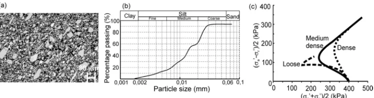
The silt investigated in this study is a non-plastic uniform silt from Vassfjellet, Klæbu,

Norway. Fig. 1a shows a backscattered electron image from an electron probe micro

analysis (EPMA) scan of a reconstituted specimen of Vassfjellet silt. Vassfjellet silt is a

medium to fine silt, it has a clay content of 2,5% and 94% of the grains have sizes lower

than 74 μm (Fig.1b).

A maximum dry density (ρd-max) of 1,6 g/cm3 was found in a Proctor compaction test at

23% optimum water content and 95% saturation. A minimum dry density was

measured by allowing a slurry to settle in a graduated cylinder (method by Bradshaw

and Baxter, 2007). Mineralogy x-ray diffraction (XRD) analysis has indicated a

composition of: 35% muscovite, 27% quartz, 18% chlorite, 15% feldspar and 5%

actinolite. High dilatant behaviour was observed in saturated samples of this material

tested in undrained triaxial tests (B-value of approximately 0,95) at its maximum

density (Kim, 2012). A friction angle ϕ’ of 32° and an effective cohesion estimated to 4

kPa are also reported by Kim (2012).

Typical failure mechanisms from undrained triaxial tests presented by Ovando-Shelley

(1986) and also observed for Vassfjellet silt (Paniagua, 2014), show that silt can exhibit

both contractive and dilative behaviour. A dilative failure mechanism, characterised by

a tendency of volume increase, causes a reduction in the pore pressure (towards

suction) in a saturated sample; while a contractive failure mechanism, characterised by

a reduction in volume, leads to an increase in the pore pressure. The resulting stress

paths show that the loose and medium dense silts contract initially before showing

dilatant behaviour, while for dense specimens the initial contraction is less obvious

(Fig. 1c).

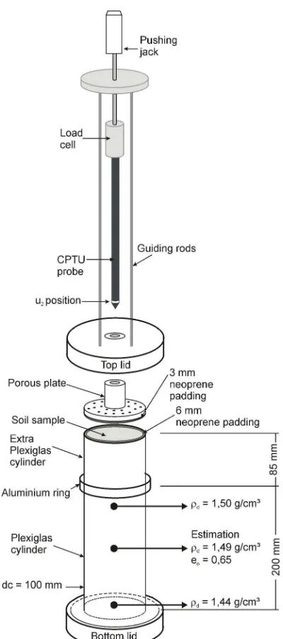
CPTU at model scale

Three specimens were prepared by the slurry consolidation method (adapted from

Kuerbis and Vaid 1988). The slurry was prepared with 45% water content and

consolidated under a top loading of 65 kPa for 12 hours. The load was applied using a

load-controlled jack that pushes a movable porous plate on top of the slurry sample

(Fig. 2). The porous plate and a filter paper allowed drainage from the top part of the

sample. The specimens were built inside a Plexiglas cylinder of 100 mm diameter and

200 mm height padded with two layers of neoprene padding of 6 mm thickness (Fig.

2). The paddings were used to compensate for the effect of the boundary closeness and

account for the compressibility of the lacking surrounding soil. The soil cylinder had a

diameter of 88 mm and a height of 180 mm. The specimens exhibited water content

and density variations with depth inherently related to the sample preparation

method. Lower water content and higher density were measured at the top of the

specimen, as water content increases and density decreases with depth. After

preparation, the samples were preloaded with 80 kPa and this load was kept during

cone penetration. The test was stopped at a penetration depth of 60 mm.

Measurements of dry density at the top and bottom of similar specimens indicated a ρd

of 1,46 g/cm³ and a corresponding experimental void ratio of 6,5 at 60 mm depth (Fig.

2).

The penetrating probe had a diameter of 12 mm and an apex angle at the tip of 60°. The

penetration force was measured in all tests at the end of the shaft, therefore, it

combines cone penetration resistance and shaft friction measurements. A pore pressure

ceramic filter was located at the position u2 (behind the cone tip) and the pore pressure

sensor was located at the end of the shaft. The pore pressure filter and sensor were

saturated under vacuum and the chamber connecting them was filled with de-aired

glycerine before penetration. The samples were penetrated at three different rates: 0,06

mm/s (slow), 6 mm/s (medium) and 50 mm/s (fast). The penetration rates were chosen

according to the recommendations of DeJong and Randolph (2012) with the aim of

obtaining a combination of drained and undrained conditions.

IMAGE ACQUISITION

Thin sections

After probe penetration, the samples were rapidly frozen with the cone inside the

sample, following the technique proposed by Paniagua et al. (2012). This set-up

permitted the cylindrical Plexiglas container and the cone to be subsequently removed

and the frozen sample to be cut through its centre. After sample cutting, the frozen

blocks were carefully oven dried based on author’s previous experience on drying

techniques. Subsequent resin impregnation was carried out both on carefully carved

smaller pieces and directly in the areas around the cone and the shaft (Gylland et al.

2013). A low viscosity epoxy resin was used to avoid disturbance of the soil

microstructure. Resin impregnation of soil for fabric inspection was successfully used

in previous studies, e.g. Fonseca et al. (2012). Thin sections of 36x22 mm and 30 μm

thick, were prepared to study the deformation zones around the cone and shaft. The

thin sections were extracted from the zones around the cone tip following 60 mm

penetration into a soil specimen 180 mm high. For the subsequent analysis it is

assumed that the silt, in this part of the sample, has initially a medium density.

Electron Probe Microscopy

The thin sections were first inspected using a polarized light microscope (Nesse, 2011)

in order to define specific areas of interest for detailed analysis using backscattered

electron images (obtained from Electron Probe Micro Analyser, EPMA, JEOL

JXA-8500F). Figure 3 shows the location of the thin sections in the specimens. SDCP stands

for Slurry Deposition Cone Penetration. The symbol # seen in Figure 3, was replaced

for each test by: S for slow penetration test (i.e. 0,06 mm/s or SDCP-S), M for medium

penetration test (6 mm/s or SDCP-M) and F for fast penetration tests (50 mm/s or

SDCP-F). The angle α refers to the angle relative to a reference plane (shown as a

thicker line) for measuring the particle orientations in the angular histograms. The

numbered dots indicate the locations where EPMA images were taken. Those locations

were selected based on previously identified deformation zones observed by Paniagua

et al. (2013). Each image is defined by 1790x2560 pixels with a pixel size of 0,4 μm

(image resolution). The high spatial resolution, as well as the good image quality, have

allowed a clear identification of the grains and pore spaces. The image processing

techniques used in this study are described in the following sections.

POROSITY ANALYSIS

Methodology

Porosity analysis from an image requires the identification of the voids or pore space,

representing air or water, and the solid particles. Binarisation by thresholding is a

commonly used technique to separate the solid from the pore space. It consists of

defining a threshold value from the bi-modal intensity distribution histogram of the

image. The result is a binary image where pixels belonging to the particles are

attributed the value 1 and pixels in the pore space are given the value 0. The threshold

value that minimizes the intra-class variance between the two classes or peaks, as

proposed by Otsu (1979), was used (algorithm implemented in ImageJ 1.48g, Rasband

2013). Measuring the void ratio value from a binary image consists of calculating the

ratio between the number of pixels corresponding to pore space and the number of

pixels associated with grains in the plane of the thin section. The 2D image-based void

ratio values were calculated for the locations presented in Figure 3. Localised artefacts

due to irregularities in the specimen surface and grain plucking resulting from thin

section preparation were avoided in the selected locations. Comparison between the

image-based and laboratory-measured void ratio of 0,65 should be done with some

reservation as the latter one is a global value that does not account for local variations

within the sample. Also to note are the limitations of using a 2D analysis to measure a

parameters that should consider the three dimensionality of the samples. While the

difference between 2D and 3D void ratio measurements have not been established for

silts, this is not likely to affect the comparative analysis for the three tests, presented

here.

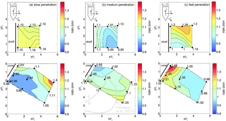
Void ratio contour plots

Figure 4 provides the void ratio distribution presented as contour plots obtained by

cubic interpolation of the measured values. The contours show an increase of the void

ratio values from the tip of the cone to outwards areas for the slow penetration rate

test, while for the fast penetration rate test an inverse trend is observed. Also, there is

no clear continuity between the values obtained for the cone and the shaft which

indicates the influence of the cone shoulder geometry. The failure zones observed by

Paniagua et al. (2013) are shown for comparison in the test with medium penetration

rate. This comparison between the void ratio contour plots and the failure zones from

Paniagua et al. (2013) can be done, noting that the results obtained in this work are

cumulative values (i.e. they are taken at the end of penetration) and the ones from

Paniagua et al. (2013) come from an incremental analysis. Besides, a cumulative

analysis of the incremental volumetric strains has shown identical results to the

incremental observations (Paniagua et al., 2013).

The lower void ratio values observed near the cone face for the slow penetration rate

test indicate that dilation along the shaft is less likely to develop at this rate. The high

void ratio values attained for the fast rate test is an indication that the dilation zone

tends to expand as the rate of penetration increases. For the medium penetration rate,

there is more variation in the porosity values along the cone face. These observations

suggest that the rate of penetration is responsible for the mobilisation of either a

contractive or dilative response near the tip of the cone with a consequent effect on the

cone resistance. In other words, for slow rate, contraction dominates the failure process

while for fast rate, dilation dominates. At an intermediate rate, the results indicate the

effect of partial drainage.

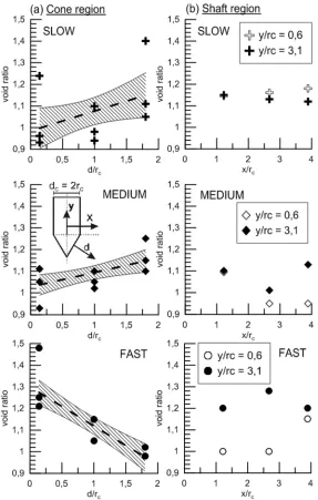
Void ratio against distance to cone

Potential patterns in the variation of void ratio around the cone were investigated.

Figure 5 shows the void ratio values for the different locations of the three tests as a

function of a normalized distance of d/rc and x/rc for the cone and shaft regions

respectively. In these plots, rc is the shaft radius, d is measured from the cone face, x is

the horizontal distance from the line of symmetry of the probe. For the slow

penetration tests, low void ratio values are observed near the cone and they tend to

increase as d/rc increases. A different pattern can be seen for the test performed at fast

penetration rate, i.e. high void ratio values are measured near the cone and they

decrease for farther regions. The rate of penetration also influences the porosity along

the shaft-shoulder region. Although no clear trend can be found for the void ratio

distribution along x/rc, faster penetration can be seen to lead to higher void ratio values

along the shaft and lower near the shoulder.

Drainage patterns

The void ratio distribution can be linked to the drainage pattern. At slow penetration

rates, drained behaviour is expected (Randolph and Hope 2004) which agrees with a

low porosity zone (i.e. contraction dominated) in Figures 5 and 6, as this rate allows the

water to drain (i.e. drained contraction). For the medium rate of penetration, the void

ratio distribution relates to the partially drained behaviour resulting from contractive

and dilative regions. The fast rate of penetration prevents the water from draining and

a dilative zone (with high porosity values) is formed, also confirmed by finite element

simulations carried out by the authors. The high void ratios observed near the cone

face are likely to contribute to the development of negative pore pressures when

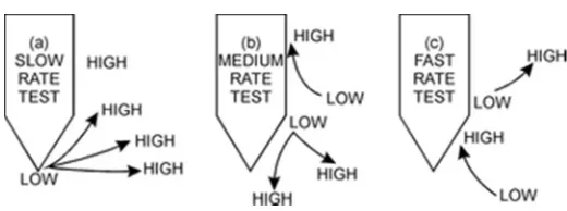
penetration occurs at fast rates, also observed by Silva (2005). Figure 6 shows schematic

diagrams of the void ratio variation around the probe where the arrows represent the

potential drainage paths, assuming that the water will travel from the low porosity to

the high porosity regions. During slow penetration there will be a side/upward

drainage from the cone tip (Figure 6a). While for the fast penetration rate, the drainage

paths are essentially upward towards the cone tip (Figure 6c). Again, for the medium

penetration rate (Figure 6b) the drainage shows a more complex pattern of paths given

the porosity variation along the cone face.

PARTICLE ORIENTATION ANALYSIS

Methodology

While for the porosity analysis the grains are treated as part of a single solid phase, the

investigation into the orientation of the grains requires the identification of the

individual grains within it, i.e. segmenting the image. This task involves more

sophisticated image processing techniques when compared to thresholding described

previously. Watershed techniques have been used for siliceous sands with relatively

rounded and convex grains (e.g. Fonseca et al. 2013a). In the case of a silt, the diversity

of particle shape ranging from almost spherical to needle-like grains and the wide

range of grain sizes, makes the segmentation process more complex. Paniagua et al.

(2014) and Fonseca et al. (2013c) describe the use of manual techniques to quantify the

characteristics of individual grains for the case of lower quality images where the

edges of the grains are difficult to identify and an automated process is not viable. In

the present study, the high quality of the EPMA images has enabled the development

of an automated process to segment the images. In order to facilitate the image

processing, grains defined by less than 30 pixels (approximately diameter of 2 µm) are

removed and assumed that their orientation is not relevant for this analysis. Note that

this corresponds to the clay fraction and represents less than 2,5% of the total grains. In

addition, the different mineralogical composition of the grains originates very distinct

intensity values representing the solid phase in the images. The process of

segmentation, consisted of 1) filtering the solid phase with similar intensity values and

2) applying a series of morphological operations consisting of eroding and dilating the

edges of the grains in order to associate to each grain a unique intensity value or ID.

The MATLAB Image Processing Toolbox (Mathworks) was used.

The second task consisted of obtaining the orientation of the major and minor axes for

each grain. This was done using the principal component analysis (PCA). PCA is

applied to the cloud of points/pixels defining each individual grain given by the x,y

coordinates and ID value (details can be found in Fonseca et al. 2013a). The orientation

of each grain (i.e. angle θ) is given by the vector describing the orientation of particle’s

major axis (Fig. 7a).

Size and shape description

The process used to obtain the size of the grains involved two key steps as developed

by Fonseca (2011): 1) orthogonal rotation of the pixel coordinates defining each grain,

so that its principal axes (obtained previously) were made parallel to the Cartesian axes

and 2) subtracting the corresponding rotated coordinates to obtain the major and

minor dimensions of the grain (Fig. 7a). The two principal axes lengths of each particle

in µm were obtained by multiplying the length given in pixels by the size of each pixel

(i.e. image resolution). The shape description of each grain was done using the aspect

ratio descriptor (AR) or elongation, given by the ratio between the lengths of the minor

and the major axes in each grain (e.g., ARsphere = 1). The statistical distribution of the AR

values is presented in Figure 7b for one of the specimens (to note that no significant

variation has been found between specimens) compared to a silica sand (Fonseca et al

2012). This silt exhibits AR values ranging from 0,1, i.e. needle-like grains, to

approximately circular grains, i.e. AR = 1; while the sand shows a much narrower

range of values, i.e. 0,6 - 1. The bias in the re-orientation of the more elongate flaky

grains under imposed deformation has been reported in previous studies (e.g. Lupini

1981). For the orientation analysis, the grains were divided into two classes according

to their AR value: i.e. bulky grains AR > 0,50 and flaky for AR < 0,50.

Angular histograms

The statistical distribution of particle orientation was investigated using 2D angular

histograms or rose diagrams. Rose diagrams provide an effective way to visualise the

distribution of a given set of vectors. In these plots the vectors are “binned" into an

interval of selected size and represented as a segment whose length is proportional to

the number of vectors orientated within the angle defining the bin limits. The

orientation of the vectors is given by the angle α measured relatively to the reference

plane shown in Figure 3, i.e. horizontal plane for the shaft and the plane inclined 32°

from the horizontal for the cone region. In the histograms, shown in Figure 8, each bin

represents an angular interval for angle α and is shaded according to either the major

axis length (in μm) or the AR to provide additional information on the link between

grain characteristics and preferential orientation. Only half of the plane is considered in

the rose diagrams since each particle has a defined orientation vector without a specific

direction, i.e. an orientation of 60° is equivalent to an orientation of 240°. These angular

plots correspond to the location SDCP-S-S1-1 and refer to all grains (Figure 8a), flaky

grains (Figure 8b) and bulky grains (Figure 8c), respectively. The orientation pattern is

similar in the three cases and the key aspect to note is the more explicit preferential

orientation of the flaky grains when compared to a more random distribution for the

bulky. It is also clear that the directional trend pattern is set by the longer and more

elongated grains, depicted by the lighter shading.

Figure 9 illustrates the distribution of particle orientation at selected locations, for all

grains after penetration and for the regions near the cone, starting from the top shaft to

the cone tip for the medium rate test, i.e. regions M-S1-1, M-S1-4,

SDCP-M-C1-4, SDCP-M-C1-3, SDCP-M-C1-2, SDCP-M-C1-1. A clear vertical orientation of

the grains major axes, i.e. parallel to the shaft, can be observed for the two positions in

the shaft region. Similar trend can be observed for the cone region where the grains

tend to re-orientate parallel to the cone face and at the tip of the cone at a

perpendicular orientation to the cone movement.

Microscale parameters

Two parameters are used for the quantitative characterisation of the distribution of

particle orientation. The first relates to the preferred orientation of the particle

distribution and is called the β value and the second parameter describes the

anisotropy of the particle distribution (A).

a) β value

This angular parameter is given by the eigenvector associated with the major

eigenvalue of the fabric tensor. The fabric tensor of the vectors defining the particle

orientations is denoted as follows (Satake, 1982):

∑

N 1

1 ₍₁₎

where N is the total number of vectors in the system, k i

n is the unit orientation vector

along direction i and k j

n is the unit orientation vector along direction j.

b) Anisotropy value

The anisotropy of the system is quantified by considering the difference between the

major and minor eigenvalues of the fabric tensor, i.e. Φ1- Φ3 (e.g. Thornton 2000,

Fonseca et al. 2013a). An isotropic distribution will have an A value of zero and the

correspondent vectors distributed equally in all directions, while the realignment of the

vectors along a preferable direction will lead to higher values of A. An effective way of

graphically representing the degree of anisotropy is to use a Fourier series (Rothenburg

and Bathurst 1989, Barreto 2008). The value of A increases with the concentration of the

orientation vectors towards a preferable angle. Two extreme anisotropy values are

presented here. Figure 10a illustrates the case of A = 0,06 (near zero) with the Fourier

fitting represented by the dotted lines, exhibiting a near circular shape. The case of A =

0,53, illustrated in Figure 10b, shows a clear preferable orientation and an associated

‘more elongated’ fitting curve. Distributions with higher anisotropy values are

characterized by a predominant particle alignment which is given by the angle β. In

more isotropic distributions, the particles tend to align in random directions and the

angle β becomes less meaningful.

Anisotropy against distance to cone

Figure 11 shows the variation of anisotropy with the normalized distance d/rc for the

cone region and x/rc for the shaft for both flaky and bulky grains. The anisotropy

values attained at the end of the test relate to the extent of realignment of the grains.

However, when compared to trends observed in Fig. 5 for porosity, it can be seen that

there is not always a direct correlation between void ratio and anisotropy values. The

test carried out at medium penetration rate, for SDCP-M in Fig.11a, suggests the

development of three areas of distinct anisotropy for the cone region based on the

rotation of the grains imposed by the cone movement. In zone 1, near to the cone, the

grains realign along the direction of the cone's face: downwards and sideward at the

tip. The interaction of these mechanisms leads to grains reorient in distinct directions,

resulting therefore, in lower anisotropy values. For zone 2, the grains follow the cone

movement but as the distance from the cone increases, a 'strong' realignment and

higher anisotropy values are observed. Finally, the zone 3 is likely to be influenced by

the friction end effects from the walls.

The anisotropy values do not show much dependency on the rate of penetration. The

results suggest that the lower penetration rate imposes more evident reorientation

(higher A) for zone 2. It can also be observed that the trend of the anisotropy values is

the same for both flaky and bulky grains but the flaky grains have much greater

values, generally twice, than the bulky grains. This can be explained by the fact that the

bulky grains are less prone to rotate when compared to more flaky grains. For the shaft

region, low anisotropy values are attained near the shoulder for the slow penetration

rate, while for medium and fast penetration rates, higher anisotropy values are

observed.

Contour plots analysis

The distribution of the β values together with the anisotropy field for the three tests is

presented in Figure 12. These contour diagrams provide an alternative illustration of

the observations made before. In particular, to note are the lower anisotropy values

near the cone tip and higher anisotropy in the middle part of the region investigated,

which results from the stronger realignment of the grains. This trend is more

pronounced for the medium rate test as shown in Figure 12.

A clear reorientation of the grains towards the vertical direction along the shaft, i.e. β

close to zero can be observed for the three tests. This trend is more pronounced for the

fast test, which also exhibits the lowest void ratio values. The grains near the cone also

align parallel to the cone face. At the cone tip the grains rotate towards an orientation

perpendicular to the cone pushing direction as a consequence of the deformation

mechanism imposed by the movement of the cone. The rate of the test does not seem to

affect significantly the final preferred orientation of the grains following penetration.

The extent of the region affected by the movement of the cone cannot be clearly

defined. Referring to Paniagua et al. (2013) no significant strains were measured

outside the regions defined by the dotted lines in Fig. 5 which would mean that

locations 7 to 10 in the cone region and 3 and 6 in the shaft region might not be

significantly influenced by penetration. As a result of the slurry deposition used to

prepare the initial sample, a near horizontal particle orientation would be expected.

The more inclined orientation deviating from the horizontal direction observed for the

grains in these outer regions is believed to a result of side friction during sample

preparation, also reported by Cetin (2004), what is known as the silo theory effect

(Janssen, 1895).

LINKING MICRO TO MACRO BEHAVIOUR

The macro response obtained for the three CPTU tests carried out on Vassfjellet silt

with a medium density is presented in Table 1. It can be seen that increasing the

penetration rate from a slow value (drained behaviour) to a medium value leads to a

reduction of the penetration resistance TR; while further increase in the rate to a fast

penetration value (approaching undrained conditions) is associated with an increase of

the penetration resistance. Regarding the pore pressure (u2), the values are seen to

decrease as the penetration rate increases and negative values are measured at both

medium and fast rates. The analysis of the local porosity has shown high void ratio

values near the cone at fast penetration rate which supports the development of

negative pore pressures due to the dilative response. For the slow penetration rate test

the lower void ratio values found near the cone tip suggest drained contraction.

Table 1. Measurements of total penetration resistance (TR) and pore pressure (u2) for the three tests carried out a different penetration rates given by the cone velocity (v)

Test v (mm/s) TR (N) u2 (kPa)

Slow SDCP-S 0,06 200 2,5

Medium SDCP-M 6 190 -10

Fast SDCP-F 50 225 -40

As discussed previously, the anisotropy of the particle orientation is believed to be

largely related to the rotation of the grains imposed by the movement of the cone and

these micro scale parameters can also be linked to the dilative response of the soil. Low

anisotropy values can be associated with zones of dilation as the grains tend to

re-orient in random directions that create a “less organised” system with larger voids and

therefore “less contractive”. Conversely, a system with a strong predominant

orientation and higher anisotropy values will be more “more contractive” (Fig. 13).

Figure 14 combines the measured observations for the medium penetration rate test,

with EPMA images with the aim of providing a more scientific explanation for the

formation of the dilative and compacted systems. It can be observed that the low

anisotropy values close to the cone tip and high void ratio agree with the dilative zone

denoted by Paniagua et al. (2013). The dilation decreases as the distance from the cone

increases making the particle distributions “more organized” and “more contractive”

towards the limit between the contractive and dilative zones identified in Paniagua et

al. (2013). At larger distances from the cone face, the randomness in the distributions

increases as well as the void ratio values. Along the shaft, the zone closer to the cone

shoulder show higher anisotropy values perhaps associated with a better alignment of

the grains at this location.

CONCLUSIONS

This paper shows that investigating soil fabric following CPTU tests, carried out on silt

at different penetration rates, can help understanding the grain-scale mechanisms,

induced by the cone penetration, that underlie the measured macroscale response. In

particular, the partial drainage behaviour can be linked to the distribution of the void

ratio and particle orientation in the regions surrounding the probe during penetration.

The analysis of local void ratio measurements allows the identification of areas with

distinct density that are, therefore, prone to exhibit distinct behaviour in terms of their

tendency to contract or dilate. Zones more prone to dilate were seen to be associated

with low anisotropy values of the vectors defining grain orientation, as the grains tend

to create a “less organised” system with larger voids within. Conversely, zones of

contraction show strong grain alignment, thus lower anisotropy values of grain

orientation and lower void ratio. It is shown that the development of regions of

contraction and dilation is influenced by the penetration rate. For higher penetration

rate, a dilative area, i.e. high void ratio, was identified near the cone, which is believed

to be associated with the generation of negative pore pressure and also leading to an

increase of cone resistance. For slow penetration rate, the low porosity values observed

near the cone indicate the tendency of this zone to contract and thus, exhibiting

drained behaviour. This study suggests that the rate-dependent response of CPTU in

silt is not only dependent on the drainage rates but is, above all, a result of the

evolution of the soil microstructure in the region surrounding the probe. The findings

herein presented show that understanding the mechanisms of grain reorientation

following cone penetration is of utmost importance to explain the drainage patterns

controlling the cone resistance and the development of pore pressures.

ACKNOWLEDGEMENTS

Workshop engineers F. Stæhli and T. Westrum at NTNU are greatly acknowledged for

valuable help with construction of the testing apparatus. Engineer A. Monsøy at

NTNU prepared the thin sections. The EPMA scans were performed by Engineer W.

Dahl at SINTEF. M. Long at University College Dublin is greatly acknowledged for

reviewing the manuscript.

REFERENCES

Barreto D., O'Sullivan c. and Zdravkovic l. 2008. Specimen generation approaches for DEM simulations. International symposium on deformation characteristics of geomaterials. Bradshaw, A.S. and Baxter, C.D.P. 2007. Sample preparation of silts for liquefaction testing.

Geotechnical Testing Journal ASTM 30: 324-332.

Broere W. 2001. Tunnel face stability and new CPT applications. PhD thesis. Delft University of Technology.

Butlanska J., Arroyo M., Gens A. and O’Sullivan C. 2014. Multi-scale analysis of cone penetration test (CPT) in a virtual calibration chamber. Canadian Geotechnical Journal 51: 51-66.

Cetin H. 2004. Soil-particle and pore orientation during consolidation of cohesive soils. Engineering Geology 73: 1-11.

Chung S.F., Randolph M.F. and Schneider J.A. 2006. Effect of penetration rate on penetrometer resistance in clay, J. of Geotechnical and GeoEnvironmental Eng, ASCE, 132(9): 1188–1196. DeJong J.T. and Randolph M.F. 2012. Influence of partial consolidation during cone penetration

on estimated soil behavior type and pore pressure dissipation measurements. Journal of Geot. and Geoenvironmental Engineering ASCE 138 (7): 777-788.

DeJong J.T., Jaeger R.A., Boulanger R.W., Randolph M.F. and Wahl D.A.J. 2013. Variable penetration rate cone testing for characterization of intermediate soils. In Countinho and Mayne (eds) Geotech. and geoph. site charact. 4. London: Taylor & Francis.

Fonseca, J. 2011. The evolution of morphology and fabric of a sand during shearing. PhD thesis. Imperial College London.

Fonseca, J., O’Sullivan, C., Coop, M. and Lee, P.D. 2012. Non-invasive characterization of particle morphology of natural sands. Soils and Foundations 52 (4): 712-722.

Fonseca, J., O’Sullivan, C., Coop, M. and Lee, P.D. 2013a. Quantifying evolution soil fabric during shearing using directional parameters. Géotechnique 63 (6): 487-499.

Fonseca, J., O’Sullivan, C., Hagira, T., Yasuda, H. and Gourlay, C.M. 2013c. In situ study granular micromechanics in semi-solid carbon steels. Acta Materialia 61 (11): 4169-4179. Gylland, A., Rueslåtten, H., Jostad, H.P. and Nordal, S. 2013. Microstructural observations shear

zones in sensitive clay. Engineering Geology 163: 75-88.

Jaeger R.A., DeJong J.T., Boulanger, R.W., Low, H.E. and Randolph, M.F. 2010. Variable penetration rate CPT in an intermediate soil. Proc., Int. Symp. on Cone Penetration Testing, Huntington Beach, CA, 8 pgs.

Janssen, H.A. 1895. Zeitschr. d. Vereines deutscher Ingenieure 39, 1045.

Jiang, M.J., Zhu, H.H. and Harris, D. 2008. Classical and non-classical kinematic fields of two-dimensional penetration tests on granular ground by discrete element method analyses. Granular Matter 10: 439-455.

Kim K., Prezzi M., Salgado R. and Lee, W. 2008. Effect of penetration rate on cone penetration resistance in saturated clayey soils, J. of Geotechnical and GeoEnvironmental Eng, ASCE, 134(8): 1142–1153.

Kim, Y. 2012. Properties of silt and CPTU in model scale. MSc project work. NTNU, Trondheim, Norway.

Kinloch H. and O’Sullivan C. 2007. A micro-mechanical study of the influence of penetrometer geometry on failure mechanisms in granular soils. Advances in measurement and modelling of soil behaviour. Geo-Denver 2007: new peaks in Geotechnics, pp. 1-11.

Kuerbis R. and Vais Y.P. 1988. Sand sample preparation – the slurry deposition method. Soils and Foundations 28 (4): 107-118.

Liu J. and Iskander M. 2010. Modelling capacity of transparent soil. Can. Geotech. J. 47, No. 4, 451–460.

Lunne, T., Robertson, P. and Powell, J. 1997. CPT in geotechnical practice. New York: Blackie Academic.

Lupini, J. F., Skinner, A. E and Vaughan, P. R. (1981). Drained residual strength of cohesive soils Géotechnique, 31 (2), p. 181-213

Muromachi T. 1974. Experimental study on application of static cone penetrometer to subsurface investigation of weak cohesive soils. ESOPT 2: 192–285.

Nesse, W. 2011. Introduction to mineralogy. Oxford University Press.

Otsu, N. 1979. A threshold selection method from gray level histograms. IEEE Transactions on Systems, Man and Cybernetics 9 (1): 62-66.

Ovando-Shelley E. 1986. Stress – strain behavior of granular soils tested in the triaxial cell. PhD thesis. University of London, Imperial College.

Paniagua, P. 2014. Model testing of cone penetration in silt with numerical simulations. PhD thesis. Norwegian University of Science and Technology, Trondheim, Norway.

Paniagua, P., Andó, E., Silva, M., Nordal, S. and Viggiani, G. 2013. Soil deformation around penetrating cone in silt. Géotechnique Letters 3: 185-191.

Paniagua, P., Fonseca, J., Gylland, A. and Nordal. 2014. Microstructural study of the deformation zones around a penetrating cone tip in silty soil. International Symposium on Geomechanics from Micro to Macro (IS-Cambridge2014).

Paniagua, P., Gylland, A. and Nordal, S. 2012. Experimental study of deformation pattern around penetrating coned tip. In Laloui & Ferrari (eds) Multiphysical testing soils-shales: 227–232. Berlin: Springer.

Poulsen R., Nielsen B.N. and Ibsen L.B. 2013. Correlation between cone penetration rate and measured cone penetration parameters in silty soils. 18th International Conference on Soil Mechanics and Geotechnical Engineering. Paris, pp. 603-606.

Randolph M.F. and Hope S. 2004. Effect of cone velocity on cone resistance and excess pore pressures, Proc., IS Osaka-Engineering Practice and Performance of Soft Deposits, Osaka, Japan, 147–152.

Rasband, W. 2013. ImageJ 1.48g. National Institutes of Health, USA.

Robinsky E.I and Morrison C.F. 1964. Sand displacement and compaction around model friction piles. Canadian Geotechnical Journal 1:81-93.

Rothenburg, L. and Bathurst, R. J. 1989 Analytical study of induced anisotropy in idealized granular materials. Géotechnique 39 (4): 601-614

Roy M., Michaud D., Tavenas F., Leroueil S. and Rochelle P.L. 1974. The interpretation of static cone penetration test in sensitive clay. ESOPT 2: 323-330.

Schneider J.A., Lehane B.M. and Schnaid, F. 2007. Velocity effects on piezocone measurements in normal and overconsolidated clays. International Journal of Physical Modelling in Geotechnics 2: 23-34.

Schneider J.A., Randolph M.F., Mayne P.W. and Ramsey N.R. 2008. Analysis of factors influencing soil classification using normalized piezocone tip resistance and pore pressure parameters. Journal of Geotechnical and Geoenvironmental Engineering 134 (11): 1569-1586. Silva M.F. 2005. Numerical and physical models of rate effects in soil penetration. PhD

dissertation. University of Cambridge.

Te Kamp, W.G.B. 1982. The influence of the rate of penetration on the cone resistance qc in sand. Proceeding of the Second European Symposium on Penetration Testing. Amsterdam: 627-633. Rotterdam: Balkema.

Thornton, C. 2000. Numerical simulations of deviatoric shear deformations of granular media. Géotechnique 50 (1): 43-53.

White D., Take W. and Bolton M. 2003. Soil deformation measurement using particle image velocimetry (PIV) and photogrammetry. Géotechnique 53 (7): 619-631.

Yafrate N.J. and DeJong J.T. 2007. Influence of Penetration Rate on Measured Resistance with Full Flow Penetrometers in Soft Clay, ASCE GI GeoDenver Conference, Denver, CO., pp. 1-10.

Yasafuku N. and Hyde A.F.L. 1995. Pile end-bearing capacity in crushable sands. Géotechnique 45: 663-676.

LIST OF FIGURES

Figure 1. (a) Backscattered electron image from EPMA scan, (b) grain size distribution of the Vassfjellet silt and (c) stress paths (adapted from Ovando-Shelley 1986).

Figure 2. Experimental set up used in the experiments presented in this paper. The variation in dry density measured and estimated in the specimen is specified.

Figure 3. Location of thin sections in the specimens studied at (a) cone region and (b) shaft region.

Figure 4. Spatial variation of void ratio values around the cone and shaft regions for (a) slow, (b) medium and (c) fast penetration rate. C: contraction and D: dilation.

Figure 5. Variation of void ratio values with the normalized distance either (a) d/rc for the cone

region or (b) x/rc for the shaft region in the different tests. The shaded area corresponds to an

80% confidence for the main trend shown (dotted line).

Figure 6. Schematic representation for the void ratio variation around the probe. The arrows show the expected drainage pattern from high pore pressures (related to low void ratios or more contraction) to low pore pressures (related to high void ratios or more dilation).

Figure 7. (a) Procedure for definition of size and shape of each grain. (b) Distribution of AR. Figure 8. Rose diagrams of particle orientations for all, flaky and bulky grains SDCP-S-S1-1. Figure 9. Rose diagrams of particle orientations of all grains for selected locations (defined in Fig. 3): (a) S1-1, (b) S1-4, (c) C1-4, (d) C1-3, (e) SDCP-M-C1-2 and (f) SDCP-M-C1-1.

Figure 10. Examples of (a) an isotropic rose diagram for bulky grains in SDCP-S-C1-10 and (b) an anisotropic rose diagram for SDCP-M-C1-5. The red discontinuous line indicates the curve fitting.

Figure 11. Variation of anisotropy with (a) d/rc (cone region) or (b) x/rc (shaft region) for flaky

and bulky grains in SDCP-S (slow rate test), SDCP-M (medium rate test) and SDCP-F (fast rate test).

Figure 12. Distribution of the angle β and spatial variation of anisotropy A of flaky grains for the zones around the cone and the shaft in (a) slow, (b) medium and (c) fast penetration rate. Each black line is oriented according to the angle β. The anisotropy values are shown at its corresponding location.

Figure 13. (a) System with grains oriented in random directions (low A) and high void ratio (dilation), (b) system with stronger grain orientation grains (high A) and low void ratio values (contraction).

Figure 14. Contours around cone and shaft of the medium penetration rate test for: (a) void ratio, (b) anisotropy and angle β. (c) Sectors of EPMA images at each location compared to Paniagua et al. (2013) observations. Each square has a side measurement equal to 80 µm. D: dilation and C: contraction.

Figure 1. (a) Backscattered electron image from EPMA scan, (b) grain size distribution of the Vassfjellet silt and (c) stress paths (adapted from Ovando-Shelley 1986).

47x12mm (600 x 600 DPI)

Figure 2. Experimental set up used in the experiments presented in this paper. The variation in dry density measured and estimated in the specimen is specified.

195x444mm (300 x 300 DPI)

Figure 3. Location of thin sections in the specimens studied at (a) cone region and (b) shaft region. 54x35mm (300 x 300 DPI)

Figure 4. Spatial variation of void ratio values around the cone and shaft regions for (a) slow, (b) medium and (c) fast penetration rate. C: contraction and D: dilation.

97x52mm (600 x 600 DPI)

Figure 5. Variation of void ratio values with the normalized distance either (a) d/rc for the cone region or (b) x/rc for the shaft region in the different tests. The shaded area corresponds to an 80% confidence for the

main trend shown (dotted line). 86x136mm (199 x 199 DPI)

Figure 6. Schematic representation for the void ratio variation around the probe. The arrows show the expected drainage pattern from high pore pressures (related to low void ratios or more contraction) to low

pore pressures (related to high void ratios or more dilation). 29x9mm (300 x 300 DPI)

Figure 7. (a) Procedure for definition of size and shape of each grain. (b) Distribution of AR. 48x12mm (300 x 300 DPI)

Figure 8. Rose diagrams of particle orientations for all, flaky and bulky grains SDCP-S-S1-1. 55x17mm (300 x 300 DPI)

Figure 9. Rose diagrams of particle orientations of all grains for selected locations (defined in Fig. 3): (a) S1-1, (b) S1-4, (c) C1-4, (d) C1-3, (e) C1-2 and (f)

SDCP-M-C1-1.

87x42mm (600 x 600 DPI)

Figure 10. Examples of (a) an isotropic rose diagram for bulky grains in SDCP-S-C1-10 and (b) an anisotropic rose diagram for SDCP-M-C1-5. The red discontinuous line indicates the curve fitting.

37x16mm (600 x 600 DPI)

Figure 11. Variation of anisotropy with (a) d/rc (cone region) or (b) x/rc (shaft region) for flaky and bulky grains in SDCP-S (slow rate test), SDCP-M (medium rate test) and SDCP-F (fast rate test).

86x106mm (199 x 199 DPI)

Figure 12. Distribution of the angle β and spatial variation of anisotropy A of flaky grains for the zones around the cone and the shaft in (a) slow, (b) medium and (c) fast penetration rate. Each black line is oriented according to the angle β. The anisotropy values are shown at its corresponding location.

98x52mm (600 x 600 DPI)

Figure 13. (a) System with grains oriented in random directions (low A) and high void ratio (dilation), (b) system with stronger grain orientation grains (high A) and low void ratio values (contraction).

37x16mm (600 x 600 DPI)

Figure 14. Contours around cone and shaft of the medium penetration rate test for: (a) void ratio, (b) anisotropy and angle β. (c) Sectors of EPMA images at each location compared to Paniagua et al. (2013)

observations. Each square has a side measurement equal to 80 µm. D: dilation and C: contraction.

98x53mm (600 x 600 DPI)