A quantitative approach to behavioural analysis of drivers in highways using particle filtering

City, University of London Institutional Repository

Citation

:

Mamouei, M. H., Kaparias, I. and Halikias, G. (2015). A quantitative approach to

behavioural analysis of drivers in highways using particle filtering. Paper presented at the

47th Annual Conference of the Universities’ Transport Study Group, 05-01-2015 -

07-01-2015, London, UK.

This is the accepted version of the paper.

This version of the publication may differ from the final published

version.

Permanent repository link:

http://openaccess.city.ac.uk/6245/

Link to published version

:

Copyright and reuse:

City Research Online aims to make research

outputs of City, University of London available to a wider audience.

Copyright and Moral Rights remain with the author(s) and/or copyright

holders. URLs from City Research Online may be freely distributed and

linked to.

City Research Online:

http://openaccess.city.ac.uk/

[email protected]

A quantitative approach to behavioural analysis of drivers in highways

using particle filtering

Mohammad Mamouei

PhD candidate,

City University London

Ioannis Kaparias

Lecturer in Transport Engineering,

City University London

George Halikias

Professor in Control Engineering,

City University London

Abstract

The analysis of the driving behaviour is a challenging area in transport that has applications in numerous fields ranging from highway design to micro-simulation and development of advanced driver assistance systems (ADAS). There has been evidence suggesting changes in the driving behaviour in response to changes in traffic conditions, and this is known as adaptive driving behaviour. Identifying these changes, the conditions under which they happen, and describing them in a systematic way would contribute greatly to the accuracy of micro-simulation and more importantly to the understanding of the traffic flow, and will therefore pave the way for introducing further improvements in the efficiency of the transport network. In this paper adaptive driving behaviour is linked to changes in the model parameters for a given car-following model. These changes are tracked using a dynamic system identification method, namely unscented particle filtering.

1. Introduction

A look at the more than six-decade-long body of studies on micro-simulation points to the difficulty of representing the dynamics of driving under different traffic conditions and for different drivers by a single mathematical equation. There have been studies reporting that the behaviour of different drivers may best be represented using different model structures (Punzo & Simonelli, 2007; Ossen & Hoogendoorn, 2007). In other words, different drivers drive according to different models. Additionally, individual drivers exhibit different driving patterns in different traffic conditions, a phenomenon that is addressed in multiple studies (Munoz & Daganzo, 2002; Ma & Andréasson, 2007; Hoogendoorn, et al., 2006). Moreover, the fact that the calibration of car-following models is highly dependent on the driving condition, as confirmed by numerous studies, such as (Punzo & Simonelli, 2007; Ossen & Hoogendoorn, 2008; Kesting & Treiber, 2009), is another indicator to adaptive driving behaviour. Many car-following models have a multi-regime structure to cope with this issue and achieve more accuracy in the reproduction of the driving behaviour, such as the models proposed by Wiedemann, Yang, and Fritzsche implemented in the VISSIM, MITSIM, and Paramics microsimulation software, respectively (Wiedemann, 1974; Yang & Koutsopoulos, 1996; Fritzsche, 1994).

well as the spacing in between the two, in order to group the data into different regimes. In (Thiemann, et al., 2008) probability density functions for headways of a large amount of trajectory data were calculated. These empirical observations point out to a significant correlation between headway and variables representing driving condition such as speed, approaching speed, and traffic condition. In (Treiber, et al., 2006) a general adaptation method that can be integrated within a wide range of car-following models was proposed. This adaptation mechanism simply states that headway in smooth traffic flow increases linearly with variations in the local traffic. A measure for representing these variations is then given and then calibrated empirically using data from a Dutch highway. In (Hoogendoorn, et al., 2006) unscented particle filtering was used to calibrate two car-following models dynamically, namely the Gazis-Herman-Rothery (GHR) and Helly models. Unlike static system identification methods, where the whole period of time series data are used to find the single set of model parameters resulting in least error, in this method parameters are allowed to vary at each time instance to minimise the estimate error. Variations in the model parameters as a function of time were provided as a yet another evidence to adaptive driving behaviour.

In this paper the possibility of utilising unscented particle filtering for a purpose beyond simple demonstration of variations in model parameters is investigated. Herein, the main research question is the investigation of the possibility of linking the changes in the model parameters to external stimuli or driving conditions. Deriving a conclusion with this regard could have two significant benefits. Firstly, such information will help gain a better insight into traffic dynamics and dynamic driving behaviour. A by-product of this is improvement in micro-simulation and modelling. Secondly, different aspects of a car-following model can be assessed based on the robustness of the parameter estimates.

The rest of this paper is organised as follows. A brief introduction on the car-following model used in this work, the calibration of car-following models, and the unscented particle filtering are given in Section 2. The simulated dataset and the application of the unscented particle filtering to this dataset are described in Section 3. Moreover, in this section a simple method for discretisation of the dynamic parameter estimates is proposed. This discretisation facilitates the identification and analysis of the dynamic driving behaviour. The proposed method is then applied to NGSIM dataset and the results are discussed in Section 4, and finally concluding notes and future work are discussed in Section 5.

2. Background

Car-following models, and acceleration models in general, represent the understanding of the behaviour of human drivers. These models, integrated in simulation software, are used to assess policy-making in various fields related to transport networks, ranging from highway design to the evaluation of advanced driver assistance systems (ADAS). However, not all of these models are developed for the same purpose, and different levels of accuracy might be required accordingly, and so different car-following models may best serve different purposes. For a review of different car-following models, the reader is referred to (Brackstone & McDonald, 1999; Ahmed, 1999).

System identification is another important aspect for car-following models. Car-following models describe the structure of stimuli-response underlying the car-following behaviour in a mathematical form. However, for application in a specific scenario the model needs to be adjusted and tailored. This may be done through calibration using an appropriate dataset.

In this section, first the car-following model used in this work, the Intelligent Driving Model (IDM), is described. Then some of the considerations related to the calibration of car-following models are discussed, and finally the method of unscented particle filtering is briefly described.

2.1. The IDM car-following model

macroscopic and microscopic calibration of the IDM model point to the good performance of this model on both aspects (Treiber, et al., 2000; Treiber & Kesting, 2013; Punzo & Simonelli, 2007). Moreover, it is computationally simple and relies on a small number of parameters, each with an intuitive meaning. Finally, numerous studies on different aspects this model such as calibration, stability and other microscopic and macroscopic properties are available (Wilson & Ward, 2011; Kesting & Treiber, 2009).

The IDM model is given by the following general equation;

where, is maximum acceleration, vd is desired speed, is acceleration exponent, s0 and s1 determine jam distances in fully stopped traffic and in high densities respectively, T is safe time headway, b is comfortable deceleration, and they are all model parameters. Input variables are speed of the subject vehicle, v, speed of the preceding vehicle, vp, and distance headway, s. Finally, the output variable, , determines the acceleration of the subject vehicle.

2.2. Calibration of car-following model

Numerous factors in the calibration of a car-following model must be taken into account. The choice of the dataset, the method employed for calibration, and the purpose for which the calibrated model is to be employed are of great importance. When a certain level of accuracy in the collective behaviour or traffic flow is required to reproduce the same flow-density characteristics as observed in real data, a certain set of model parameters for a given car-following model may work best ( Treiber, et al., 2000). However, for the purpose of modelling microscopic behaviour of individual drivers, including details such as velocity and spacing of individual vehicles, a different set of model parameters may work best (Treiber & Kesting, 2013). Even for a single driver a significant inconsistency between calibration results for different trajectory data is found. This means that if one intends to reproduce accurate trajectories for a specific driving condition, for a given driver, while driving in a stretch of a specific highway, e.g. upstream of a bottleneck, taking into account the traffic flow and density, weather condition, etc., the data used for calibration must match the scenario under investigation in terms of traffic characteristics.

Even excluding the question of intra-driver inconsistencies, this gives rise to the so called phenomenon of over-fitting. Over-fitting means that the model will be so accurately adapted to a given scenario that it will lose its generality, such that for an only slightly different driving scenario the results would be completely inaccurate and consequently unreliable for making any predictions. One may recognise this as a trade-off between accuracy and robust calibration. Other considerations regarding calibration include the choice of: error measurement, e.g. travel time, spacing, velocity, acceleration; system identification method, e.g. Maximum-Likelihood Estimation (MLE), Least Squares Estimation (LSE), and nonlinear optimisation methods such as Genetic Algorithm; and finally error tests, e.g., Root Mean Square error (RMSe), Root Mean Square Percentage error (RMSQe), and Theil’s inequality coefficient (U). For a review on some of these considerations, the reader is referred to (Punzo & Simonelli, 2007; Ossen & Hoogendoorn, 2008; Treiber & Kesting, 2013; Ranjitkar, et al., 2004).

2.3. Unscented particle filtering

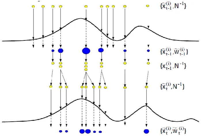
et al. 2000). Figure 1 gives a schematic representation of this method.

Figure 1 illustration of the three stages of importance sampling, resampling, and sampling (prediction) in PF, figure from (van der Merwe et al. 2000)

For more details and pseudo-code of the method refer to (van der Merwe et al. 2000; Hoogendoorn et al. 2006; Arulampalam et al. 2002).

3. Methodology

In this section, a brief on the simulated dataset is provided. The unscented particle filtering is then applied to the simulated data to investigate the extent to which the properties of the adaptive driving can be identified using this method. Moreover, the choice of the objective function for calibration is described. Finally, a simple method for discretisation of the estimates is proposed. The discretisation of the dynamic estimates is an important step to make sense of the raw estimates obtained initially and link the changes in the model parameter to the traffic conditions.

3.1. Simulated dataset

In the previous section, unscented particle filtering was introduced. In this section the application of this method to simulated data is investigated to illustrate the extent to which this method can be utilised for the purpose of “meaningful” dynamic calibration of car-following models. The additional constraint arising from the term “meaningful” refers to the fact that, sometimes by calibrating a number of model parameters simultaneously, an error in the estimation of one model parameter may be compensated by another error (over-estimation or under-(over-estimation depending on the relation between the two model parameters) in estimation of the other model parameters. This happens due to the fact that the information available is less than what is required for the determination of the unknowns, and in this sense it is similar to trying to find the solution to a system of three linear equations with four unknowns. The lack of independent information on the fourth equation results in infinite possible solutions instead of the unique solution intended.

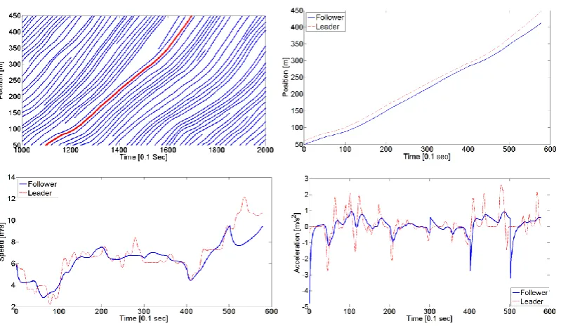
Figure 2 a) Trajectory of the lead vehicle selected from NGSIM data Lane 2 b,c,d) Position trajectories, velocities, and accelerations of the lead vehicle and synthetized follower in dashed

red line and blue line respectively

The parameter profiles used for the simulation of the trajectories shown are as follows. The default model parameters reported by (Treiber, Hennecke, & Helbing 2000) are used up to Time t=300. At this instance, the following parameters are changed to the given values:

.

Additionally, the value of the parameter, T, changes again to the values T=1 and T=3 at time points t=400 and t=500, respectively.

3.2. Application of unscented particle filtering to simulated data

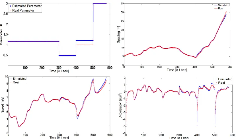
Figure 3 shows the results of the application of the method to the simulated dataset. For this purpose, all of the model parameters are set to their default values, except for parameter T, which is to be estimated.

Figure 3 The result for estimation of the parameter T. The blue shadow denotes the distribution of particles at each time instance while the red curve is the selected particle.

It can be seen that up to time t=300, the estimation of parameter T is almost error-free and stable. Also, the subsequent changes at the times t=300, t=400, and t=500 can be identified from Figure 3 by “jumps” in the values of the parameter at these times, compared to the smooth curves in the intervals between the changes. The estimations of parameter T at times after t=300, unlike before, are unstable and fluctuate around a certain value. This is due to the fact that beyond time t=300 other model parameters were changed to values other than the ones used in the estimation process. As a result, the effect of this false estimation needs to be compensated for by overestimations and underestimations of parameter T.

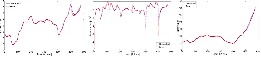
Using the parameter estimation given by the application of unscented particle filtering (Figure 3), almost perfect estimation of the spacing ( ), velocity ( ) and acceleration ( ) can be derived despite the error in other model parameters from t=300 afterwards). This is shown in Figure 4.

Figure 4 The comparison of real trajectories with simulated trajectories when the dynamic estimation of the parameter T, given by unscented particle filtering, is used.

It should be noted that herein, the IDM car-following model was used to generate trajectories for the follower vehicles, and the same car-following model was used in the calibration process. In the application to real data, this is the equivalent of assuming knowledge of the model underlying the behaviour of human drivers. Although this is obviously not the case, the findings of (Ossen & Hoogendoorn, 2008) may justify use of such simulated data. Therein, it was found that the characteristics of the followers’ behaviour can be recovered by calibrating a car-following model to data, even when the real model is different than the model used for calibration.

3.3. Objective function

(RMSPe). For more details on this subject, the reader is referred to (Punzo & Simonelli, 2007; Ossen & Hoogendoorn, 2008; Treiber & Kesting, 2013; Ranjitkar, et al., 2004).

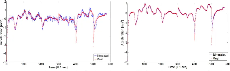
In (Punzo & Simonelli, 2007), the inter-vehicle spacing was suggested as the most reliable MOP. In this work, however, it was found that the best result is obtained when a combination of errors on spacing, velocity, and acceleration was used in the objective function instead of selecting a single variable as the performance measure. This might be due to utilising the information available on all variables. Herein, the weighted sum of squared errors on all the three variables was used. The accuracy of the acceleration trajectories in NGSIM data is somewhat questionable, as pointed out by (Thiemann, Treiber , & Kesting, 2008) nonetheless, excluding acceleration error between the predicted values and real values from the objective function results in randomly fluctuating estimates of acceleration with unrealistically large values for jerk. This can be avoided by including acceleration error in the objective function with a low weight to suppress significant influence of these inaccurate data on the estimation process. Figure below, illustrates the simulated acceleration trajectory when acceleration error is excluded from the objective function. Although in this case a slight improvement in the simulated velocity and spacing trajectories is obtained yet, as it can be seen from Fig. 5 this improvements comes at the great cost for acceleration.

Figure 5 Comparison of the simulated accelerations with the real values when acceleration error is a) excluded in the objective function b) included in the objective function

3.4. Making sense of the dynamic parameter estimates

As was shown in Figure 3, although the “jumps” in the value of the model parameters are visually identifiable, when the method is applied to real data the resulting estimates are much harder to interpret. This makes the identification of the points where a sudden change in the model parameter takes place difficult, and is due to two reasons: 1) the actual changes in the model parameters are not known in advance; and 2) the changes are much less intense and more frequent. As one would expect from human drivers, they do not drive in a crisp and deterministic fashion, and neither do they immediately change their underlying incentives as soon as they reach a different traffic condition, but instead a smooth and gradual change in incentives is to be expected from them. Moreover, it should be pointed out that for real data, the true underlying model generating the car-following dynamics is unknown.

comparison of the simulated results using this method compared to the real data.

Figure 6. Comparison of the simulated trajectories when averaging between the breaking points is applied with real results for a) The estimation of parameter T b) Spacing c)Speed

d)Acceleration

It can be seen that not only the points where the parameter is changed are identified correctly, but also the values of the parameter within corresponding intervals are estimated with relatively high accuracy. Hence, the acceleration, velocity, and spacing trajectories are generated with accuracy that is incomparable to any static estimation method.

4. Results

In the previous section it was shown that using the unscented particle filtering along with the proposed discretisation method, the changes in the model parameters can be identified and consequently the changes in the driving behaviour can be captured. In this section, this method is applied to the NGSIM trajectory dataset to investigate the question of the identification of the adaptive driving behaviour.

4.1. Application to the NGSIM dataset

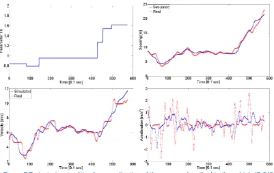
The functionality of the proposed method was illustrated using simulated data. In this section the proposed method is applied to a platoon of nine vehicles driving in the second lane to investigate the following two issues: 1) whether the assumption of systematic changes in driving incentives can be validated; and 2) whether these changes can be identified using car-following models, such as IDM, and an adaptive system identification method, such as unscented particle filtering. All the vehicles observed remain in the platoon for the whole duration of the experiment, and this means that the dynamics are not disturbed by lane changes. Figure 7 illustrates the application of the proposed method to one of the vehicles. The first figure illustrates the discretised parameter estimate. This parameter profile is subsequently used to simulate the driving behaviour for the follower. The comparison of the simulated states (spacing, speed, and acceleration) with the real states points to the accuracy of the simulated behaviour. The reason why the acceleration estimates are relatively poor is due to the low weight of this variable in the objective function as explained earlier.

Figure 7 Trajectories resulting from application of the proposed method to the vehicle ID 348

4.2. Analysis of the parameter estimates

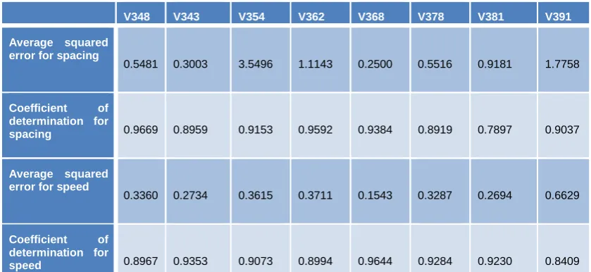
Figure 8 illustrates the resulting parameter estimates for the vehicles, based on which very accurate estimates of the spacing and and velocity trajectories can be obtained. Table 1 summarises the errors in estimation of velocity and spacing.

V348 V343 V354 V362 V368 V378 V381 V391

Average squared error for spacing

0.5481 0.3003

3.5496 1.1143 0.2500 0.5516 0.9181 1.7758

Coefficient of

determination for

spacing 0.9669

0.8959 0.9153 0.9592 0.9384 0.8919 0.7897 0.9037

Average squared error for speed

0.3360 0.2734

0.3615 0.3711 0.1543 0.3287 0.2694 0.6629

Coefficient of

determination for

speed 0.8967 0.9353 0.9073 0.8994 0.9644 0.9284 0.9230 0.8409

One of the interesting findings of this work is that in four of the eight investigated vehicles, a significant correlation between the average speed and the estimation of parameter T can be observed. Correlation between this parameter and the local average speed was also reported by (Treiber, Kesting, & Helbing 2006), and based on this, a general model that can be integrated within a number of car-following models was proposed. However, interestingly, two other distinct patterns can be observed within the estimates for this platoon: 1) the inverse relation with the average speed, as is the case with vehicle 368; and 2) irrelevant or no changes in the estimated parameter with respect to average speed, which is the case for vehicles 343, 378, and 381. Similar patterns were observed in many other examined vehicles, and the reason is likely to be difference in driving styles, intentions (such as the preparation for performing a lane change), or maybe a more complicated relation between the average speed and spacing. Further investigation on these topics and application of the method to more trajectories will shed more light on some of these issues.

5. Conclusion and future work

In this paper, unscented particle filtering was utilised to examine the dynamic behaviour of drivers in different traffic conditions. In order to interpret the estimates given by the unscented particle filtering, a simple discretisation method was used, and promising results from its application to simulated and real data were obtained. This helped to isolate minor fluctuations, which could be due to the fuzzy and stochastic nature of human driving, or minor errors in the modelling of car-following behaviour, and to convert the raw estimates given by the unscented particle filtering to an interpretable form.

The application of this method to real data delivered interesting results. Specifically, for a large number of cases, a strong correlation between average speed and the parameter under investigation was observed. This correlation was also reported by (Treiber, Kesting, & Helbing 2006). However, two additional patterns were, interestingly, observed: 1) inverse relation with the average speed; and 2) the parameter estimate is not influenced by the average speed. In spite of these, though, the employed framework has been found to have great potential in investigating the properties of traffic flow, as well as in examining the robustness and performance of car-following models.

References

Kesting, A. & Treiber, M., 2009. Calibrating Car-Following Models by Using Trajectory Data: Methodological Study. Transportation Research Record: Journal of the Transportation

Research Board, Volume 2088, pp. 148-156.

Treiber, M., Hennecke, A. & Helbing, D., 2000. Congested traffic states in empirical

observations and microscopic simulations. Physical Review E , 62(2), p. 1805–1824. Ahmed, K. I., 1999. Modeling drivers' acceleration and lane changing behavior, Cambridge,

Massachusetts: Massachusetts Institute of Technology.

Arulampalam, M. S., Maskell, S., Gordon , N. & Clapp, T., 2002. A tutorial on particle filters for online nonlinear/non-Gaussian Bayesian tracking. IEEE Transactions on Signal

Processing, 50(2), pp. 174-188.

Brackstone, M. & McDonald, M., 1999. Car-following: a historical review. Transportation

Research Part F: Traffic Psychology and Behaviour, 2(4), p. 181–196.

Brockfeld, E., Kühne, R. D. & Wagner, P., 2003. Calibration and validation of microscopic

traffic flow models. Washington, D.C., s.n.

Fritzsche, H., 1994. A model for traffic simulation. Traffic Engineering and Control, p. 317– 321.

Hoogendoorn , S. & Hoogendoorn , R., 2010. Calibration of microscopic traffic-flow models using multiple data sources. Philosophical Transactions of the Royal Society A:

Mathematical, Physical and Engineering Sciences, 368( 1928), p. 4497–4517.

Hoogendoorn, S., Ossen, S., Schreuder , M. & Gorte, B., 2006. Unscented Particle Filter for

Delayed Car-Following Models Estimation. Toronto, Canada, s.n.

Ma, X. & Andréasson, I., 2007. Behavior Measurement, Analysis, and Regime Classification in Car Following. IEEE TRANSACTIONS ON INTELLIGENT TRANSPORTATION

SYSTEMS, 8(1), pp. 144-156.

Montanino, M. & Punzo, V., 2013. Reconstructed NGSIM I80-1. COST ACTION TU0903 -

MULTITUDE. [Online]

Available at: http://www.multitude-project.eu/exchange/101.html.

MUNOZ, . J. C. & Daganzo, C. F., 2002. MOVING BOTTLENECKS: A THEORY

GROUNDED ON EXPERIMENTAL OBSERVATION. Adelaide, Australia, s.n., pp.

441-461.

Ossen , S. & Hoogendoorn, S., 2008. Calibrating car-following models using microscopic

trajectory data, Delft, Netherlands: Delft University of Technology.

Ossen, S. & Hoogendoorn, S. P., 2007. Car-following behavior analysis from microscopic trajectory data. Transportation Research Record: Journal of the Transportation

Research Board, Volume Volume 1934 / 2005 Traffic Flow Theory 2005, pp. 13-21.

Punzo, V. & Simonelli, F., 2007. Analysis and comparison of microscopic traffic flow models with real traffic microscopic data. Transportation Research Record: Journal of the

Transportation Research Board, 1934(1), pp. 53-63.

Ranjitkar, P., Nakatsuji, T. & Asano, M., 2004. Performance Evaluation of Microscopic Traffic Flow Models with Test Track Data. Transportation Research Record: Journal of the

Transportation Research Board, 1876 (1), pp. 90-100.

Thiemann, C., Treiber , M. & Kesting, A., 2008. Estimating Acceleration and Lane-Changing Dynamics Based on NGSIM Trajectory Data. Transportation Research Record:

Journal of the Transportation Research Board, Volume 2088, pp. 90-101.

Treiber, M. & Kesting, A., 2013. Microscopic Calibration and Validation of Car-Following

Models – A Systematic Approach. Noordwijk, Netherlands, s.n., p. 922–939.

Treiber, M., Kesting, A. & Helbing, D., 2006. Understanding widely scattered traffic flows, the capacity drop, and platoons as effects of variance-driven time gaps. Phys. Rev. E, 74(1), p. 016123.

van der Merwe , R., Doucet, A., de Freitas, N. & Wan, E., 2000. The Unscented Particle Filter. [Online]

filter, Technical Report CUED/F-INFENG/TR 380, , s.l.: Cambridge University Engineering Department.

Wiedemann, R., 1974. Simulation des Strassenverkehrsflusses, Karlsruhe, Germany: Schriftenreihe des Instituts für Verkehrswesen der Universität Karlsruhe, Band 8. Wilson, R. E. & Ward, J. A., 2011. Car-following models: fifty years of linear stability analysis

– a mathematical perspective. Transportation Planning and Technology, 34(1), pp. 3-18.