Implicit surfaces for interactive graph based cavity analysis of molecular simulations

City, University of London Institutional Repository

Citation:

Parulek, J., Turkay, C., Reuter, N. and Viola, I. (2012). Implicit surfaces for

interactive graph based cavity analysis of molecular simulations. Paper presented at the 2nd

IEEE Symposium on Biological Data Visualization, 14 Dec - 15 Dec 2012, Seattle, USA.

This is the unspecified version of the paper.

This version of the publication may differ from the final published

version.

Permanent repository link:

http://openaccess.city.ac.uk/3615/

Link to published version:

Copyright and reuse: City Research Online aims to make research

outputs of City, University of London available to a wider audience.

Copyright and Moral Rights remain with the author(s) and/or copyright

holders. URLs from City Research Online may be freely distributed and

linked to.

City Research Online:

http://openaccess.city.ac.uk/

[email protected]

Implicit Surfaces for Interactive Graph Based Cavity Analysis

of Molecular Simulations

Julius Parulek∗

University of Bergen

Cagatay Turkay† University of Bergen

Nathalie Reuter‡ University of Bergen

Ivan Viola§ University of Bergen

ABSTRACT

Molecular surfaces provide a suitable way to analyze and to study the evolution and interaction of molecules. The analysis is often concerned with visual identification of binding sites of ligands to a host macromolecule. We present a novel technique that is based on implicit representation, which extracts all potential binding sites and allows an advanced 3Dvisualization of these sites in the con-text of the molecule. We utilize implicit function sampling strategy to obtain potential cavity samples and graph algorithms to extract arbitrary cavity components defined by simple graphs. Moreover, we propose how to interactively visualize these graphs in the con-text of the molecular surface. We also introduce a system of linked views depicting various graph parameters that are used to perform a more elaborative study on created graphs.

Index Terms: J.3 [Computer Applications]: Life and Medi-cal Sciences—Biology and Genetics; I.3.4 [Computer Graphics]: Computational Geometry and Object Modeling—Boundary repre-sentations, Curve, surface, solid, and object representations

1 INTRODUCTION

The research field of computational molecular biology is conduct-ing discoveries about molecular machinery of life on the high-est magnification level. Molecular interactions are often studied through analysis of molecular dynamics (MD) simulation based on classical mechanics and Newtons laws of motion. The simulations result in large datasets, called trajectories and containing the se-quence of molecular structures as they vary along the simulation time. Comparison of these reveal their transformations over time.

The exploratory process is often concerned with visual identifi-cation of binding sites of ligands to a host macromolecule. For this purpose, molecular visualization conveys the molecular structure so that the binding sites can be located through the process of vi-sual analysis. For easier perception of a potential binding site such as a pocket, cavity, or a tunnel, depth-enhancing illumination mod-els are utilized. Such an approach, however, still requires a much trained eye of the domain analyst.

Complementary to these approaches, several non-visual analytic methods have been developed that allocate possible binding sites by means of analysis of the geometrical structure of the molecular model [2, 34]. The structure can be for example analyzed through stochastic seeding strategies, where the seed-point positioning can determine available area for binding. Other methods, like Voronoi diagram partitioning or discretization into a volumetric regular grid, makes segmentation techniques possible to be facilitated. The latter techniques are unfortunately often limited in identification of inter-nal tunnels and pockets, while shallow binding sites on the surface might remain undetected.

∗_{e-mail: [email protected]}

†_{e-mail: [email protected]} ‡_{e-mail: [email protected]} §_{e-mail: [email protected]}

Most of all visual and geometrical methods, however, are con-cerned with analysis of a static geometry, instead of a more physically-plausible dynamical picture such as the one provided by MD trajectories. With such an approach, a binding site that is valid only during a limited time interval is very difficult to identify and the entire approach is highly dependent on analysts intuition when selecting a particular frame.

The approach presented in this paper aims at a novel combina-tion of both visual and stochastic analysis. Moreover, the entire temporal sequence is analyzed instead of a single frame. To iden-tify binding sites, a stochastic seeding process is first applied on an implicit representation of the molecular structure. Mutual visibil-ity of seeding points (samples) is utilized to cluster the seed-points belonging to a potential binding site. The site is represented by a sparse skeleton that is extracted with existing graph algorithms. The evolution of potential binding sites can be visually analyzed over the entire temporal sequence by integrating the extracted skeleton with contextual surface representation of the molecule. Moreover, graph analysis allows us to quantitatively characterize the binding site topology and size extends.

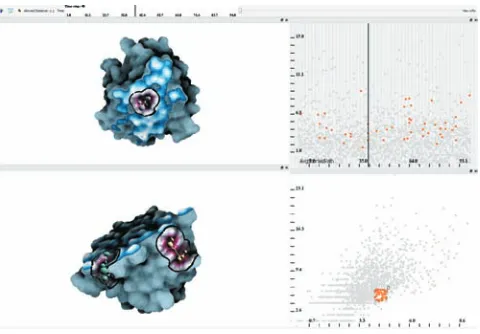
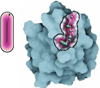
An important contribution is that we do not consider only posi-tion of atoms solely, like for instance in many Voronoi diagram ap-proaches [19, 26, 35], but instead we put emphasis on the molecular surface itself. Additionally, thanks to implicit representation we are not bound to any fixed structure, as for instance in grid based dis-cretization [14, 27, 34], but we are able to evaluate cavity distance parameters at any point in space with respect to the molecular iso-surface. Finally, the cavities are explored by means of graphs rep-resenting the potential cavity sites, which can be visually explored via linked views depicting various graph parameters (Fig. 1).

2 RELATEDWORK

We relate our work to two areas. Firstly, we introduce techniques of implicit molecular representation. Secondly, we describe cavity extraction techniques.

2.1 Implicit Representation of Molecules

Implicit surfaces provide a suitable way to easily model complex dynamically changing geometric objects. In the area of molecular visualization, they find their stable place, mainly because of their ability to model smooth bond transitions between individual atoms. The set of techniques, known today as implicit modeling, was used for the first time by Blinn [1]. He introduced the implicit function, describing the electron density function of atoms, by summing the contribution from each atom as follows:

f(p) =T−

∑

i

bie−aid

2

i_{, (1)}

wheredirepresents the distance frompto the center of atomi,bi

represents the ”blobbiness”,aidescribes the atom radius andT

de-fines the electron density threshold. Later on several different rep-resentations of implicit surfaces, built up from skeleton points, were introduced [22, 36]. The general formula for these representations is defined as:

f(p) =T−

∑

i

mifi(p), (2)

wheremiis a weighting factor and fiis a decreasing density

dis-tribution function defined as: fi=hi◦di, wherehi (e.g., ear

2

in Eq. 1) is a kernel function anddirepresents the distance to atom

i. Comparative analysis of application of different kernel functions was introduced in [31]. The efficient GPU implementation of ker-nel evaluation in the rendering pipeline was introduced by Kolb and Cuntz [12]. Similar approaches were later introduced for fast molecular visualization [5, 14]. Although the approaches based on summation of atom contributions are fast to compute, they do not fully take into account the solvent (represented usually by sphere of radiusR), which can reveal the possible binding sites on the molecule. Nevertheless, they are being still well-used and preferred techniques in molecular visualization.

Pasko et al. [24] generalized the representation of implicit sur-faces, by combination of the different forms of implicit models, and denoted it as function representation. The inequality (3) describes an implicit solid (object):

f(p)≥0, (3)

wherep= (x1,x2,x3)∈E3. Function f is called an implicit

sur-face function (implicit function), which classifies the space into two half-spaces f(p)>0 and f(p)<0. This classification applies to Eqs. 1 and 2 as well. Besides summation, complex objects can be created from individual components via Constructive Solid Geom-etry (CSG) operations. The basic set-theoretic operations can be defined using theminandmaxoperators:

f1∪f2 = max(f1,f2)

f1∩f2 = min(f1,f2) (4)

Analytical expressions that approximate these operators were pro-posed by Ricci [29].

In the literature, there are several types of molecular surface rep-resentations, where one of the basic one is when the protein atoms are depicted as spheres, where the radius corresponds to the van der Waals force (vdW surface) [16]. When denoting atom centers as

ciand their van der Waals radii as ri, the van der Waals implicit

function fulfilling Eq. 3 is defined as: f(p) =∪i(ri−di). Solvent

accessible surface (SAS) is then obtained by the extension of this surface by a solvent radiusR: f(p) =∪i((ri+R)−di).

The most widely used representation, with respect to cavity ex-ploration, is denoted as solvent excluded surface (SES) [30]. The recent GPU implementation of SES representation visualization was proposed by Lindow et al. [19] and Krone et al. [13]. Al-though the rendering performance is high, their models can be used for rendering purposes solely. Moreover, in our work, we delimit ourselves to representations that define the molecule as an implicit surface, which is a prerequisite for our cavity detection technique.

The modeling and visualization of theSES representation by means of functional representation was introduced by Parulek and Viola [23]. The authors represent the molecular surface via com-bination of basicCSGoperators, Eq. 4, to create a distance based implicit function. We take this representation as a basis for the function sampling procedure. However, itsO(n3)complexity dur-ing the function evaluation step causes non-competitive renderdur-ing performance for bigger proteins; i.e., below 10 FPS. Therefore, to get the interactive rendering performance we utilized a simplified surface representation, which on one hand provides a fast render-ing performance, but on the other hand only approximates theSES. The more detailed description is in Section 3.3.

In order to visualize implicit molecular models, one can convert them to a mesh representation prior to rendering them as a set of patch primitives [20]. The major drawback is when we deal with complex molecular models, one would need to generate millions of triangles to obtain a fully detailed iso-surface. Therefore, in recent years, several techniques have been introduced that exploit direct visualization methods, represented by ray-casting methods. One subclass of implicit surfaces are represented by distance based functions. Effective visualization of such objects was proposed by Hart [8]. Since, essentially, the distance measure for an implicit function can be approximated by the first Newton iteration of the function:

fdist(p)≈

f(p)

|∇F(p)|; (5)

we also adopted Hart’s technique for rendering.

The recent studies address ray-casting of general implicit sur-faces on GPU using interval arithmetics [10] and via so-called adaptive marching point method [32]. However, these methods are aimed at globally defined functions, which is not often the case of molecules, where the function is usually evaluated based on the neighboring atoms solely; i.e.; only taking into account those atoms that lie in the close vicinity of the evaluated point. Naturally, when using for instance Eq. 1, the kernel function has an infinite domain of influence. In such a case all the molecule atoms should be con-sidered.

2.2 Protein Cavity Analysis

Due to the valuable information provided by empty spaces formed by protein surfaces, analysis of cavities and tunnels have been stud-ied widely. In 1983, Connolly [3] proposed an analytical descrip-tion of theSES representation, which was utilized by Voss and Gerstein in their web-based cavity analysis tool [35]. They apply two distinct probes to determine the solvent volume where potential cavities and channels may reside.

al. use Voronoi diagrams to discover molecular channels and pores. Recently Lindow et al. [18] presented a technique that allows to ex-tract significants paths from the molecules. In their approach the authors utilize Voronoi diagram of spheres. Additionally, the edges of Voronoi diagrams lying outside the domain of the molecule were removed by a set of random rays generated at Voronoi vertices. This method resembles our technique; nevertheless we do not employ Voronoi vertices, but rather implicit function sampling that empha-sizes the molecular surface. Their final visualization was achieved by means of placing light sources on the extracted paths.

An iterative and heuristic algorithm is used in PoreWalker [25] to determine channels using pore features. Our method, with respect to tunnel extraction techniques, can be thought of as combination of stochastic methods (function sampling) and Voronoi diagrams (graph analysis).

Another set of approaches aim at extraction and analysis of molecular pockets and cavities. In 1998, Liang et al. [17] intro-duced a program CAST that uses computational geometry methods and alpha shape theory to extract cavities. In McVol [34] Till and Ullmann describe a Monte Carlo algorithm to sample the protein surface in a 3D grid. Essentially, this approach is similar to ours, where the main difference being that the authors use a 3Dregular grid and does not allow for interactive visual analysis. Recently, Raunest et al. [28] introduced a grid-based approach that also con-siders molecular dynamics to identify internal cavities and tunnels. In 2011, Krone et al. [14] introduce a method to track the cavity evolution over time. A user selects a cavity that is then tracked for each frame. The authors voxelize the implicit function into a 3D

volume grid, which is subsequently segmented by means of the 3D

flood fill method. In our work, we employ monte carlo function sampling strategy to utilize directly the molecular surface informa-tion to extract potential cavities. We do not track cavities over time, but rather form a large set of potential cavities for every time step independently, where a user is provided by linked views that allow her to explore the space of cavities with respect to 3Dmolecular visualization.

3 METHODOVERVIEW

We assume that a molecule is represented by an implicit function

f(p). One can use a kernel based approach (Eq. 2), or the one pro-posed in [23]. The required function properties include: a) the im-plicit function is positive inside the molecule and negative outside, b) it is possible to estimate the minimum distance from a sample point. The second requirement can be achieved by application of Newton’s formula, Eq. 5. It is important to mention that in this paper, we do not focus on describing the best possible implicit rep-resentation, but rather we aim at the method to extract all possible cavities and the corresponding visualization. Nevertheless, differ-ent choices of the function forms yield to differdiffer-ent results naturally. Our method computes an independent set of graphs,Gt={Gt₁∪

. . .∪Gtm}, representing possible cavities of MD simulation in time

stept. In order to construct graphaGt, we firstly populate the defini-tion space of the molecule, defined by the bounded box of time step

t, by random samples. The implicit function is evaluated at every sample position, where all the samples that lie inside the molecule or farther away from the surface than the user defined threshold are discarded. Secondly, the samples are then filtered to delimit them only to those that might possibly lie inside the cavity. This is per-formed by tracing a ray from every sample following the gradient of the function obtained at the sample point. When the ray hits the surface, the sample is labeled as potential cavity sample and its po-sition is updated accordingly. Thirdly, the mutual visibility test be-tween pairs of cavity samples is performed. This yields to 3Dgraph formation, where each mutually visible pair defines an edge in the graph. Afterwards, we perform independent component analysis of the graph, which results in an independent set of graph components

Gt. We also perform the minimum spanning tree algorithm to every independent graph component to obtain its central skeleton.

We visualize the graph components using basic geometrical el-ements, where we employ spheres for nodes and line segments for edges. The molecular visualization is performed with respect to the selected graph components. Additionally, we introduce a new im-plicit clipping plane for molecules. Here, we utilize the fact that the function evaluation is done during the scene ray-casting, which allows us to clip-away atoms used for function evaluation, which lie in front of the clipping plane. The user is provided with linked views allowing her to select individual graphs according to various graph properties.

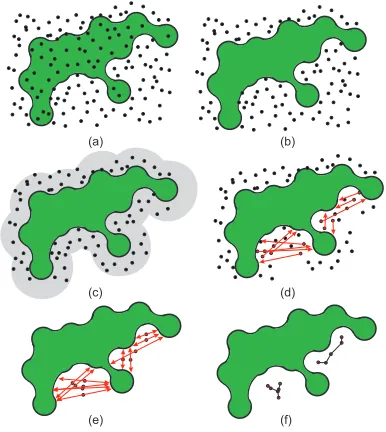
3.1 Cavity Sample Points

In the first stage, we sample the implicit functions by a set of ran-dom points,S={p1, . . . ,pn}, which densely cover the function

do-main (Fig. 2a). For simplicity, the dodo-main is represented by the protein bounding box. We perform the sampling for every time step of MD simulation, where the position of sampling points re-main almost the same for all the time steps, i.e.; we slightly adjust the position with respect to the molecule bounding box in a par-ticular time step. The number of points (samples) that are seeded to the scene depends primarily on the size of the molecule, where for instance for Proteinase 3, used in our use case containing 3346 atoms, we used 30K of sample points. Essentially, the sampling process evaluates the implicit function fat every sample position, which can be done in parallel, at each time step independently; i.e., we obtain a set of function valuesFt_={f(p

1), . . . ,f(pn)}for time

(a)

(c) (d)

(b)

(e) (f)

stept. The sampling is performed in the precomputation for all MD trajectories.

With respect to the property of implicit functions that classifies points between internal and external ones, we can easily filter out samplesS0⊆Sthat lie inside the protein,S0={p|f(p)≤0p∈S

(Fig. 2b). After discarding samples that lie inside the molecule, still many samples might remain. Therefore, we filter out even more samples, by removing all the samples that lie farther away from the surface. We introduce parameterDrepresenting the maximum al-lowed distance from the samples to the molecular surface. In our work, after discussion with biologists, we set this value to 2R; i.e.; all the samples that lie within a solvent diameter range. More for-mally, we define the set as

S1={p|f(p)≤ −2R∧p∈(S−S0)}, (6)

where an exemplified scenario is illustrated in Figure 2c. Here we generate a set containing sample points lying in a close vicinity to the surface. Please note that the number of samples inS1depends

on the surface complexity predominantly.

As a next step, we perform a cavity based analysis, which classi-fies the samples into potential cavity samples. By normalization of the function gradientN(p) =∇f(p)/|∇f(p)|, we obtain a normal direction to the molecular surface. Here for every sample a ray is cast along the normal direction, beginning at the sample, and when the ray hits the surface, the sample is classified as a potential cavity sample; i.e;

Cav(p)≡[∃tp>0|f(p+tpN(p)) =0]. (7)

To evaluate the predicateCav, we use the same method that is em-ployed in the actual 3Dray-casting (see Section 3.3). Here, for all the samples that fulfilCav(p)≡1 (Fig. 2d), we compute two sur-face projections,pAandpB, along the normal, which are defined as

follows:

pA=p−fdist(p)N(p) (8)

pB=p+tpN(p), (9)

where fdist(p)is by Eq. 5. These two points are used to adjust the

sample position to lie in the middle of the line segment defined now bypA andpB, p= (pA+pB)/2 (Fig. 2e). We denote the newly

constructed set of samples asS2. Moreover, we specify a radius for

the sample as follows:

rp=min(|

pA+pB|

2 ,|fdist(p)|), (10) where fdist(p) computes the estimated minimum distance to the

surface in the new sample position. The radiusrpgives us an

esti-mation about the cavity span at the sample position. Note that using this approach we obtain samples forming both internal cavities of the molecule and also the external surface pockets.

The ray-casting method used to evaluate cavity samples can be performed in a more robust way, like for instance producing multi-ple rays in random directions. Nevertheless, casting just a single ray is a very fast method and, when taking into account the large num-ber of employed seeds, also it helps to filter out many samples in

S1. SetS2now contains a set of samples lying in the middle of two

different parts of the molecular iso-surface separated by an empty space (Fig. 3). In the previous steps, all the samples are evaluated in parallel using CUDA, where for instance evaluating and segment-ing of 30Ksamples for 100 time steps takes around one minute.

3.2 Cavity Graphs

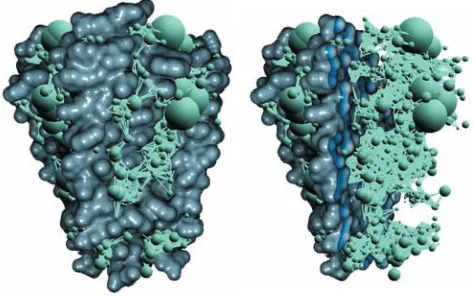
Here our goal is to form a graph that defines relations between the cavity samples. First, we perform visibility tests between all pairs

Figure 3: Visualization of cavity samples for a water channel (Aqua-porin) (left). In order to see also the interior samples, we applied an implicit clipping plane (right), introduced later in Section 3.3.1. The radii of spheres is determined by Eq. 10.

of sample points inS2. This enables us to generate an undirected

graphG, where nodes being the sample points inS2. An edge

be-tween two samples is added to the graph only if there is no visible surface between these two samples. Formally, there is no edge be-tween two samples,pandq, only if the function has at least one root, on the line segment connecting both samples. We encode this property into the predicateRoot(p,q)≡1:

Root(p,q)≡[∃t|f(p+t(q−p))≥0]. (11) In order to compute the predicate, we utilize the bisection method, also called binary search method. The line segment, defined within the interval[p,q], is recursively halved and the midpoint is tested against the positive function value. By denoting the midpoint

Hp,q=p+₂q of line segment[p,q], the bisection method is defined

by

Root(p,q)≡     

True i f |p,q|<Lmin,

False i f |p,q|>Lmax

f(Hp,q)<0∧

∧Root(p,Hp,q)∧Root(Hp,q,q) otherwise

(12) whereLmax defines the maximum allowed distance between two

samples andLminrepresents the minimum length of the tested

in-terval. The function is initialized withRoot(pi,pj). The illustration

of the algorithm is depicted in Figure 4a. Note that parameterLmin

represent the precision when searching for possible surface inter-sections. In all our demonstrations, we specifyL=0.1R; i.e., 10% of solvent radius. On the other side parameterLmaxrepresents the

maximum edge length that might be added to the graph. The ac-tual values of this parameter may vary according to what are we after. For instance, when the goal is to detect tunnels this values should be higher. While for smaller pockets on the outer molecu-lar iso-surface, this value should not be very high in order not to merge two or more distinct regions. ThusLmaxcan be thought of as

a minimum distance separating two mutually visible components. After performing all the tests, we add an edge(pi,pj)to graph

Gonly ifRoot(pi,pj)≡1, where we also specify the edge weight

as|pipj|. An example of such a graph is shown in Figure 5. After

Figure 4: A demonstration of the visibility test. The bisection method recursively halves the interval, evaluating the red point, the blue point and, finally the yellow one, which lies in the object. TheRoot predi-cate therefore equalsFalse.

To support more interactivity, which was requested by our bio-logical partners, when creating the set of independent graphs, we introduce filtering of ”weak” nodes of input graphG. Here, before applying CCA, we discard nodes, for which the number of incident edges is less thanDegmin. This parameter allows us to eliminate

weak connections between larger groups that are subjects of cavity leaking. The actual value of this parameter is difficult to determine, since there is no real default number of incident edges per a cavity node. Therefore we introduce it as a free parameter (realized by a slider), which can be interactively adjusted for each time step sep-arately. The interactive feedback of our system is preserved, since the initial graphGhas been already formed. Naturally, when hav-ing the initial graph very large (order of thousands of nodes), the response time might be in order of seconds. For instance, the gen-eration of graphs takes around 30 seconds for 100 time steps.

Sequentially, we apply minimum spanning tree algorithm [15] to each componentGito build its central skeleton (Fig. 2f). A

span-ning tree is an undirected graph whose edges are structured as a tree while the minimum spanning tree (MST) is the least of them with respect to the total sum of edge weights, represented by the distances. The MST algorithm enables us to reduce the majority of edges for each graph component, keeping just the essential ones.

Figure 5: An example of the constructed graph for potassium chan-nel (KCSA, left) with the implicit clipping plane applied (right). For illustration purposes, we specified considerably high value forLmax,

Lmax=10R, which causes a lot of graph edges being added to the

graph. The generated graph contains29686of edges and2276of nodes.

3.3 Visualization

The rendering of implicit surfaces representing molecules by a sin-gle distance based function was introduced by Parulek and Vi-ola [23]. We improved the proposed pipeline in order to get more interactive rendering performance. The implicit surface is visual-ized through the ray-casting method performed in parallel on GPU (CUDA). In the paper, for each ray, the entry and exit points were computed by means of intersection of the ray with the bounding box of the bounded molecule. This, however, led to a lot of empty spaces needed to be traversed by the ray. Therefore, instead, we uti-lize geometry shader to quickly splat billboards representing atoms as spheres(ci,ri), whereci represents the atom center andriits

radius. These are extended by solvent diameter 2R; i.e; spheres de-fined by(ci,ri+2R)are rendered. The method describing the fast

sphere rendering is presented by Lampe et al. [4]. Nevertheless, instead of rendering the spheres we store minimum and maximum depth values for each fragment performed in one rendering pass. This is done using OpenGL blending by specification of the blend-ing function to max while writblend-ing(depth,−depth)to the rendering target. For more details, we refer to a paper by Falk at al. [5], where the authors already utilized a similar approach to render a set of par-ticles defined by a kernel function.

Afterwards, by means of both computed depth values (tmin,tmax),

the first hit ray traversal is performed. A generated ray, starting at

tmin, is processed in a step-wise fashion until thetmaxis reached or

we hit the iso-surface. The ray-casting procedure increments the ray parametertby−fdist, since the function has negative values

out-side, i.e.ti+1=ti−fdist. The intersection point of the iso-surface

with the ray we denote asps. Finally, we perform the shading com-putation and enhance the depth perception by means of screen space ambient occlusion [21].

3.3.1 Implicit Clipping Plane

To allow interactive molecule exploration, we include a clipping plane, which we refer to as implicit clipping plane (ICP). ICP clips the atoms the implicit surface function is built from. Here we utilize the fact that the implicit function is constructed on the fly during the ray-casting. ICP neglects those atomscithat lie farther away

from the clipping plane thanri(Fig. 6a); i.e;d(ICP,ci)≥ −ri. We

denote the implicit surface function, implementing this constrain, by fICP(p).

Additionally, when the implicit clipping plane is activated, the shading is evaluated according to the distance of the plane to the intersection point,d(CP,ps), acquired during the ray-casting. Es-sentially, the color is computed as an interpolation of the distance within the intervald(CIP,ps)∈[−R,2R], where all computed in-tersection points beyond 2Rfrom the plane are shaded by the same color. We employ the color brewer scheme [7] spanning from white to blue tones (Fig. 6b). Users can either link the plane normal with the viewing direction, or adjust the plane orientation interactively.

3.3.2 Graph Components

The graph components are visualized using basic geometrical prim-itives (spheres and line segments), where each independent compo-nent has its own color. The radii of spheres are defined by Eq. 10. The spheres represent the nodes of each graphGk, where its edges,

after applying the minimum spanning tree algorithm, are visualized using basic line segments connecting the nodes. Our system allows to select and visualize a group of graphs per different time steps separately.

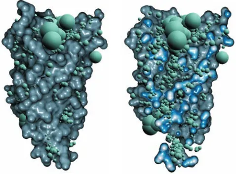
To enhance the graph components in the context of the molecule, we color the iso-surface via the minimum distance ofpsto the se-lected graph components; i.e.; their edges (Fig. 7). This distance is specified by the user as Dg, which can be arbitrarily adjusted

specifi-(b) (a)

Figure 6: Implicit clipping plane. a) The implicit function evaluates the molecular surface (green). It takes into account only atoms that inter-sect the plane or lie in the half-space defined by the plane (arrows). b) Protein Pr3 is colored according to the distance to the plane, where within range[−R,2R]the final color is interpolated as it is sketched by the blue rectangles in (a).

cation is defined as follows:

d(ps,Gi)

Dg ≤

1 (13)

whered(ps,Gk)represents the distance of iso-surface intersection

pointps to graphGi, while fulfillingd(ps,Gk)≤Dg. Moreover,

when any of the graph components is shown, we discard the shad-ing model for all iso-surface pointsps that are beyondDg; i.e.,

d(ps,Gk)>Dg (Fig. 7 right). In our demonstration we specify

Dg=3R.

Additionally, in order to preserve the primary iso-surface of function f(p), when the implicit clipping plane is applied, both functions must fulfil fICP(ps) =0= f(ps). This property is

checked during evaluation of Eq. 13, which defines whether the (clipped) iso-surface represents the iso-surface of f(p)as well. If this is not the case, the shading of those iso-surface points is done as in Figure 8.

Figure 7: Visualization of graph components. Left: The iso-surface point (the black circle), obtained during ray-casting, is evaluated against the distance to the graph component (the dashed line). This can be regarded as a distance field (shades of pink) defined by the skeleton (black). Right: An example of graph component visualiza-tion in the context of the molecule. When graph component is shown, the Phong shading model is applied only to points that lie withinDg

distance from the graph. The graph component is displayed using line segments (edges) and spheres (nodes).

Figure 8: Translation of the implicit clipping plane through the cavity, from the viewer towards the center of the molecule (left to right). In order to improve perception of the clipped iso-surface inside the cav-ity, we color the clipped parts, within distanceDgwhere fICP(ps)̸=

fICP(ps), by a monotone red color.

4 ANALYSIS OFPROTEINASE3

Proteinase 3 is an enzyme involved in inflammation. It belongs to the family of serine proteases, cleaving proteins via the hydrolysis of specific peptide bonds. In a number of chronic inflammatory dis-eases such as the Wegener granulomatosis and vasculitis, Proteinase 3 becomes too active and has a deleterious effect. It is thus a drug target. Designing drugs for Proteinase 3 implies to understand how its protein targets bind to it, so that the drug candidates developed are able to compete with the protein targets and bind stronger than these [6].

The quest for new drugs to prevent the pathological dysfunction of a given enzyme often relies on knowledge of the three dimen-sional structure of the enzyme involved, and in particular of the cavities on its surface. The efficacy of the drug candidates is in-deed dependent on a strong interaction with the enzyme and this is achieved by binding into a cavity. Proteins, like all molecules, are dynamic and the structural changes they undergo impact their function. This is also valid for the dynamics of cavities.

Here, we apply our approach to the analysis of trajectories ob-tained from molecular dynamics simulations of Proteinase 3 (Pr3) bound to a short protein. We visually analyze the structure of the protein to determine the cavities, which are likely to be the potential binding sites. We classified them to distinct categories according to the visual analysis. Our analysis involves an initial processing step followed by an interactive analysis phase.

The analysis starts with importing thePDBandDCDfiles for Pr3. The Protein Data BankPDBfile format stores the protein in-formation (e.g., atom types, residual sequences) andDCDfile for-mat, a standard format used in Visual Molecular Dynamics (VMD) tool [9], stores the atom trajectories.

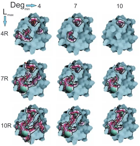
As the first step, the implicit function sampling is performed. This is done using CUDA, where all samples per a time step are evaluated byf(p)in parallel as was introduced in Section 3.1. Once the procedure is finished, the graph analysis is performed (Sec. 3.2). It is possible to regulate the graph generation step through the use of parameters. The number of graph components obtained for every time step can become very high, ifDegminis set too low. For

in-stance, setting theDegminparameter (Sec. 3.2) to 2 solely discards

single nodes, thus resulting in a high number of components. On the other hand, high values ofLmax can produce too many graph

edges, which leads to less number of graph components with many nodes. Therefore the user has the possibility to adjust freely these two parameter to increase/decrease the size and the number of com-ponents. The impact of changing parametersDegmin andLmax is

showcased in Figure 9.

4.1 Analysis setup

over-4R

4

7R

7

10R

10

L

Deg

Figure 9: An example of the effect of increasing parametersDegmin

andLmaxto connected components analysis of protein Pr3. From left

to right:Degmin=4,Degmin=7andDegmin=10. From top to bottom:

Lmax=4R,Lmax=7RandLmax=10R.

come this, we enable the visual investigation and selection of the graph components to steer the focus of the analysis. In order to interactively analyze the graph components, a number of measures are computed consequently to the graph generation step. Here we utilize a number of basic measures to quantify the properties of components to be able to compare them. For each component, we compute: the longest path between any two nodes (maxLength), the average of the shortest paths between the nodes (avgP), and the av-erage of the degree of all the nodes (degree). Note that the existing literature [11] on graph analysis offers a wide range of measures, which would make this analysis more elaborative. However, these studies are beyond the scope of this paper and can be thought of as a future extension.

At this stage, we introduce two accompanying scatterplots that visualize the quantitative measures for the graph components over time. In one (Fig. 1 top-right), we show a selected graph measure (y-axis) over time (x-axis). The other (Fig. 1 bottom-right) depicts two graph measures as opposed to each other for all the time steps. The user can select (brush) desired components over time, where in the accompanied 3Dview the selected graphs are visualized. Ad-ditionally, multiple instances of these plots can be utilized, where each one visualizes one of three graph component measures. Dif-ferent selections can be combined via the basic boolean operators.

4.2 Analysis phase

After the graph components are formed, we bring up two afore-mentioned scatterplots, one depicting parametersmaxLengthand

degreeagainst each other (A, Fig. 10) and the other showing pa-rameteravgPover time (B, Fig. 11 containing plot A as well).

Plot A depicts values that represent the graph length, being its maximum path length, with respect to the average degree of all nodes in it. By interactively selecting different components we identified three essential groups. The first one that has high

maxLength and low degree values, represents long and straight components (with very few branching structures). The second one with mediummaxLengthand lowdegreevalues, stands for more compact components having bigger span on the protein surface. The third one is represented by mediummaxLengthand high de-greevalues, which represent cavities that go much deeper into the protein.

Plot B assists in understanding the temporal location of selected components with respect toavgPvalues representing the extent of the graphs. Plot B is linked with plot A in a way that we can observe the distribution of selected components over time. Here we were able to locate components of interest very quickly and, additionally even track them over time (Fig. 11).

Figure 10: An example of scatterplot utilization. The plot (middle) shows two graph computed parameters (maxLengthanddegree), which by performing interactive selections in accordance with the3D linked visualization allowed us to identify three different graph com-ponent groups (circles).

5 FUTUREWORK

There are several ways to focus our future goals on. One task that was demanded by our biological collaborators was to track graph components over time. Possible scenarios of graph developments cover mainly splitting and merging of graph components between sequential time steps. One way would be to apply graph clustering algorithms that would automatically lead to the first results. Nev-ertheless, this would require more deeper studies with respect to graph algorithms.

Another challenge is represented by incorporating charges into the existing concept. Electron potential charges are usually solved on the discrete volumetric grid by means of solving PDE. Since the implicit representation evaluates the function values anyway for any point in space, both representations can be easily merged. The obtained charges can be then mapped both to the graph component and to the iso-surface of the molecule.

One way to analyze to evolution of graph components between neighboring time steps, is to exploit directly the implicit represen-tations, for both time steps, by building the third function that rep-resents interpolation between both two, and evaluate inter-sample visibility tests between sequential time steps.

ACKNOWLEDGEMENTS

This work has been carried out within the PhysioIllustration re-search project (# 218023), which is funded by the Norwegian Research Council. Additionally, we would like to thank Helwig Hauser and Visualization group in Bergen for useful ideas and feed-back.

REFERENCES

[1] J. Blinn. A generalization of algebraic surface drawing.ACM Trans-actions on Graphics, 1:235–256, 1982.

[2] R. Coleman and K. Sharp. Finding and characterizing tunnels in

macromolecules with application to ion channels and pores. Biophys-ical journal, 96(2):632–645, 2009.

[3] M. Connolly. Analytical molecular surface calculation. Journal of

Applied Crystallography, 16(5):548–558, 1983.

[4] O. Daae Lampe, I. Viola, N. Reuter, and H. Hauser. Two-level ap-proach to efficient visualization of protein dynamics. IEEE transac-tions on visualization and computer graphics, 13(6):1616–23, 2007. [5] M. Falk, S. Grottel, and T. Ertl. Interactive image-space volume

visu-alization for dynamic particle simulations. InProceedings of The An-nual SIGRAD Conference, pages 35–43. Link¨oping University Elec-tronic Press, 2010.

[6] E. Hajjar, B. Korkmaz, F. Gauthier, B. Brandsdal, V. Witko-Sarsat, and N. Reuter. Inspection of the binding sites of proteinase3 for the design of a highly specific substrate. Journal of medicinal chemistry, 49(4):1248–1260, 2006.

[7] M. Harrower and C. Brewer. Colorbrewer.org: An online tool for selecting colour schemes for maps. Cartographic Journal, pages 27– 37, 2003.

[8] J. C. Hart. Sphere tracing: A geometric method for the antialiased ray tracing of implicit surfaces.The Visual Computer, 12:527–545, 1994. [9] W. Humphrey, A. Dalke, and K. Schulten. VMD: visual molecular

dynamics.Journal of molecular graphics, 1(14):33–38, 1996. [10] A. Knoll, Y. Hijazi, A. Kensler, M. Schott, C. Hansen, and H.

Ha-gen. Fast Ray Tracing of Arbitrary Implicit Surfaces with Interval

and Affine Arithmetic.Computer Graphics Forum, 28(1):26–40, Mar.

2009.

[11] E. Kolaczyk.Statistical analysis of network data: methods and mod-els. Springer Verlag, 2009.

[12] A. Kolb and N. Cuntz. InProc. 18th Symposium on Simulation

Tech-nique, number Section 2, pages 722–727.

[13] M. Krone, K. Bidmon, and T. Ertl. Interactive visualization of molec-ular surface dynamics. IEEE transactions on visualization and com-puter graphics, 15(6):1391–8, 2009.

[14] M. Krone, M. Falk, and S. Rehm. Interactive Exploration of Protein

Cavities.Computer Graphics Forum, 30(3):673–682, 2011.

[15] J. B. Kruskal. On the shortest spanning subtree of a graph and the

trav-eling salesman problem. Proceedings of the American Mathematical

Society, 7(1):48–50, 1956.

[16] B. Lee and F. M. Richards. The interpretation of protein

struc-tures: estimation of static accessibility.Journal of molecular biology, 55(3):379–400, Feb. 1971.

[17] J. Liang, H. Edelsbrunner, and C. Woodward. Anatomy of protein pockets and cavities: measurement of binding site geometry and im-plications for ligand design.Protein Science, 7:1884–1897, 1998. [18] N. Lindow, D. Baum, and H.-C. Hege. Voronoi-based extraction and

visualization of molecular paths. IEEE Trans. Vis. Comput. Graph., 17(12):2025–2034, 2011.

[19] N. Lindow, D. Baum, S. Prohaska, and H.-C. Hege. Accelerated

Vi-sualization of Dynamic Molecular Surfaces. InComputer Graphics

Forum, volume 29, pages 943–952. Wiley Online Library, 2010. [20] W. E. Lorensen and H. E. Cline. Marching cubes: A high resolution 3d

surface construction algorithm.SIGGRAPH Comput. Graph., 21:163–

169, August 1987.

[21] T. Luft, C. Colditz, and O. Deussen. Image enhancement by

un-sharp masking the depth buffer. ACM Transactions on Graphics,

25(3):1206–1213, jul 2006.

[22] H. Nishimura, M. Hirai, T. Kavai, T. Kawata, I. Shirakawa, and K. Omura. Object modeling by distribution function and a method of image generation.Transactions of IECE, J68-D(4):718–725, 1985. [23] J. Parulek and I. Viola. Implicit representation of molecular surfaces. InProceedings of the IEEE Pacific Visualization Symposium (Paci-ficVis 2012), pages 217–224, March 2012.

[24] A. Pasko, V. Adzhiev, A. Sourin, and V. V. Savchenko. Function rep-resentation in geometric modeling: concepts, implementation and ap-plications.The Visual Computer, 11(8):429–446, 1995.

[25] M. Pellegrini-Calace, T. Maiwald, and J. Thornton. Porewalker: a novel tool for the identification and characterization of channels in transmembrane proteins from their three-dimensional structure.PLoS computational biology, 5(7):e1000440, 2009.

[26] M. Petˇrek, P. Kosinov´a, J. Koca, and M. Otyepka. Mole: a voronoi diagram-based explorer of molecular channels, pores, and tunnels. Structure, 15(11):1357–1363, 2007.

[27] M. Petˇrek, M. Otyepka, P. Ban´aˇs, P. Koˇsinov´a, J. Koˇca, and J. Damborsk´y. Caver: a new tool to explore routes from protein clefts, pockets and cavities.BMC bioinformatics, 7(1):316, 2006.

[28] M. Raunest and C. Kandt. dxtuber: Detecting protein cavities, tunnels and clefts based on protein and solvent dynamics.Journal of Molecu-lar Graphics and Modelling, 29(7):895 – 905, 2011.

[29] A. Ricci. A constructive geometry for computer graphics.The

Com-puter Journal, 16(2):157–160, 1972.

[30] F. M. Richards. Areas, volumes, packing, and protein structure. An-nual Review of Biophysics and Bioengineering, 6(1):151–176, 1977. [31] A. Sherstyuk. Kernel functions in convolution surfaces: a comparative

analysis.The Visual Computer, 15(4):171–182, 1999.

[32] J. M. Singh and P. J. Narayanan. Real-time ray tracing of implicit

sur-faces on the GPU. IEEE transactions on visualization and computer

graphics, 16(2):261–72, 2010.

[33] O. Smart, J. Neduvelil, X. Wang, B. Wallace, and M. Sansom. Hole: a program for the analysis of the pore dimensions of ion channel struc-tural models.Journal of molecular graphics, 14(6):354–360, 1996. [34] M. Till and G. Ullmann. Mcvol-a program for calculating protein

volumes and identifying cavities by a monte carlo algorithm.Journal of molecular modeling, 16(3):419–429, 2010.

[35] N. Voss and M. Gerstein. 3v: cavity, channel and cleft volume calcu-lator and extractor.Nucleic acids research, 38(suppl 2):W555–W562, 2010.