The SPAIR method : Isolating incident and reflected directional wave spectra in multidirectional wave basins

The SPAIR method: Isolating incident and re

fl

ected directional wave

spectra in multidirectional wave basins

S. Draycott

⁎

, T. Davey

, D.M. Ingram

, A. Day

, L. Johanning

FloWave Ocean Energy Research Facility, Max Born Crescent, King's Buildings, Edinburgh EH9 3BF, UK

b_{Institute for Energy Systems, School of Engineering, The University of Edinburgh, Edinburgh EH9 3JL, UK} c

Naval Architecture and Marine Engineering, The University of Strathclyde, Glasgow G4 0LZ, UK

d

Renewable Energy Research Group, University of Exeter, TR10 9E, UK

a b s t r a c t

a r t i c l e i n f o

Article history:

Received 3 June 2015

Received in revised form 6 April 2016 Accepted 9 April 2016

Available online xxxx

Wave tank tests aiming to reproduce realistic or site specific conditions will commonly involve using directionally spread, short-crested sea states. The measurement of these directional characteristics is required for the purposes of calibrating and validating the modelled sea state. Commonly used methods of directional spectrum reconstruction, based on directional spreading functions, have an inherent level of uncertainty associated with them. In this paper we aim to reduce the uncertainty in directional spectrum validation by introducing the SPAIR (Single-summation PTPD Approach with In-line Reflections) method, in combination with a directional wave gauge array. A variety of wave conditions were generated in the FloWave Ocean Energy Research Facility, Edinburgh, UK, to obtain a range of sea state and reflection scenarios. The presented approach is found to provide improved estimates of directional spectra over standard methods, reducing the mean apparent directional deviation down to below 6% over the range of sea states. Additionally, the method isolates incident and reflected spectra in both the frequency and time domain, and can separate these wave systems over 360°. The accuracy of the method is shown to be only slightly sensitive to the level of in-line reflection present, but at present cannot deal with oblique reflections. The SPAIR method, as presented or with slight modification, will allow complex directional sea states to be validated more effectively, enabling multidirectional wave basins to simulate realistic wave scenarios with increased confidence.

© 2016 The Authors. Published by Elsevier B.V. This is an open access article under the CC BY license (http://creativecommons.org/licenses/by/4.0/). Keywords:

SPAIR Tank testing

Directional spectrum measurement FloWave

Phase-Time-Path-Difference Wave reflection

Single-summation method

1. Introduction

Wave tank tests facilitate the understanding of how complex sea

conditions influence the dynamics of man-made structures. A key

requirement for any test programme is the ability to create these conditions in a highly controlled and repeatable manner. To have such control, it is vital to be able to measure and validate the desired test conditions. Whilst this is a relatively simple task when generating uni-directional waves, the extension to the measurement and validation of directional spectra can be challenging.

The experimental measurements presented here were made at the FloWave Ocean Energy Research Facility, located at the University of

Ed-inburgh (Fig. 1). The facility consists of a circular 25 m diameter, 2 m

depth combined wave and current test basin which is encircled by 168 active-absorbing force-feedback wavemakers. This geometry and de-sign are intended to remove any inherent limitation on wave direction and therefore allow the recreation of highly spread and highly complex

directional spectra. As such, it presents an ideal environment to explore and demonstrate directional measurement methodologies.

To validate a directional spectrum, a method of reconstruction is re-quired. Most of these methods aim to resolve the frequency-dependent Directional Spreading Function (DSF), thus describing the distribution of wave energy with direction. These methods use the measured cross-spectra between wave gauges, along with the known gauge

posi-tions, tofit a directional distribution. There are a number of approaches

in doing this, with some commonly used approaches being the Bayesian

Directional Method (BDM) (Hashimoto and Konbune, 1988), the

Maximum Likelihood Method (MLM) (Benoit et al., 1997; Krogstad,

1988), and the Extended Maximum Entropy Principal (EMEP)

(Hashimoto et al., 1994).

The nature of DSF-based reconstruction methods means that there is some uncertainty associated with the estimate. In this work we use a combined wave generation-measurement approach that enables the directional spectra to be estimated with increased certainty, whilst

additionally enabling the isolation of incident and reflected components

under certain conditions. This method has been named SPAIR, or the

Single-summation PTPD Approach with In-line Reflections, and enables

directional sea states to be validated with greater confidence.

Coastal Engineering xxx (2016) xxx–xxx

⁎ Corresponding author.

E-mail address:[email protected](S. Draycott).

http://dx.doi.org/10.1016/j.coastaleng.2016.04.012

0378-3839/© 2016 The Authors. Published by Elsevier B.V. This is an open access article under the CC BY license (http://creativecommons.org/licenses/by/4.0/).

Contents lists available atScienceDirect

Coastal Engineering

To generate the waves a single-summation method is used (Miles and Funke, 1989) ensuring that each discrete frequency component only has one propagation direction. This enables meaningful frequency dependent wave directions to be inferred from a wave gauge array,

using a Phase-Time-Path-Difference (PTPD) approach (Esteva, 1976),

providing an estimate of the directional spectrum. This approach is

demonstrated byDraycott et al. (2015), and has been shown to be

significantly more effective than both the EMEP and BDM methods at

estimating directional spectra when combined with single-summation wave generation. In this paper the method is demonstrated over a larger test matrix, designed to explore the reconstruction effectiveness over a range of peak frequencies, directional spreading and peak steepness.

Additional complex spectra are explored, which highlight the bene_fit

of using this approach when analysing highly spread or multi-modal spectra.

The SPAIR method, as employed in FloWave, uses the PTPD

ap-proach and calculated directions to perform in-line reflection

analy-sis using a least squares method, similar toZelt and Skjelbreia

(1992). Under the assumption that reflections mirror the incident,

this enables the reflected directional spectrum to be isolated, with

phase information, enabling both incident and reflected time-series

to be reconstructed.

Limits of the method assumptions are explored, particularly relating

how the magnitude and angle of reflections affect both the incident

angle calculation, and on the separation of incident and reflected

components. In addition, alternative uses of these single-summation based tools are discussed for different purposes, and for when the SPAIR method assumptions are inappropriate.

2. Methodology

2.1. Sea state input and generation

2.1.1. Input sea states

To examine the SPAIR method performance under a range of repre-sentative conditions, 27 parametric sea states were created and tested

at the facility. These tests cover a range of peak frequencies,fp, directional

spreading,s, and peak wave steepness',sp(defined asHm0/Lp, whereHm0

is the significant wave height, andLpis the peak wavelength). All of the

sea states were created using JONSWAP spectra with a constant gamma value of 3.3. In addition to this, a range of mean directions were then

considered, examining the influence of the wave gauge orientation on

the method performance. Finally three complex sea states were created, using combinations of parametric seas to provide unconventional wave conditions; both multi-modal and highly spread. The wave parameters

for these sea states are shown inTables 1, 2 and 3.

The complex sea states inTable 3have been designed to prove that

the method can reconstruct such spectra, whilst additionally isolating

the incident and reflected components over 360°. Thefirst spectrum is

a multi-modal sea state consisting of two identical wave systems with the mean direction 120° apart, whilst the second spectrum is a single wave system with a very large directional spread, spanning 360°. Two completely opposing wave systems have been used for spectrum three, with a slight difference in peak frequency. These spectra are

illustrated inFig. 17. It is often difficult to isolate the different incident

modes of such spectra using conventional methods, and the isolation of

the incident and reflected spectra is not usually possible at all without a

defined incident range. These tests therefore serve as a useful

demon-stration of the capability of the SPAIR approach used here.

2.1.2. Wave generation

Deterministic waves are generated at FloWave using force-feedback

wavemakers, providing a very high degree of repeatability (Ingram et al.,

2014). This enables device alterations to be assessed independently

of sea state variations, and allows wave-by-wave comparisons to be made of the device in the time domain.

Throughout this work the generation of directional wave spectra is achieved using the single-summation method, avoiding phase-locking (Miles and Funke, 1989). Phase-locking occurs when waves at the same frequency but different directions interact, causing spatial

patterns across the tank, thus creating a non-ergodic wavefield. To

avoid this, the initial frequency increments,ΔF, can be split up further

to create sub-frequency incrementsδf =ΔF/Nθ, as shown inPascal

(2012). These new frequency increments, still within the original frequency bins, now have a unique wave propagation direction associ-ated with each of them. In addition to avoiding phase-locking, this method of wave generation is key to the application of the SPAIR

method. This generation approach is demonstrated inFig. 2.

Using the re-defined directional spectrum, the surface elevation can

be calculated via an Inverse Fast Fourier Transform (IFFT), or summation.

The surface elevation at point [x,y], and timetcan now be described by:

ηðx;y;tÞ ¼ X

NfNθ−1

i¼0

Aicosð−ωitþki½xcosαiþysinαi þΦiÞ ð1Þ

where:

Ai wave amplitude of frequency componenti

ωi angular frequency of componenti, rad/s

ki ¼2Lπi, wavenumber of componenti

Fig. 1.The FloWave Ocean Energy Research Facility.

Table 1

Main 3×3×3 test matrix (27 tests in total).

Wave parameter Range of values

Peak frequency,fp[Hz] 0.45 0.6 0.75

cos-2 s spreading value,s 5 10 25

Peak steepness [%] 1 2 4

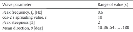
Table 2

Directional sensitivity tests (10 tests in total).

Wave parameter Range of value(s)

Peak frequency,fp[Hz] 0.6

cos-2 s spreading value,s 10

Peak steepness [%] 2

Mean direction,θ[deg] 18 , 36 , 54 ,…, 180

Table 3

Complex spectra tests.

Wave parameter Spec 1 Spec 2 Spec 3

Peak frequency,fp[Hz] 0.5, 0.5 0.45 0.45, 0.55

αi wave direction of componenti

Φi phase of componentiatx=y=t= 0.

The sea states presented here have a repeat time, T, of 1024 s. This

defines the frequency increments,δf, to be 1

1024Hz, providing 2048

frequency components within the tank's nominal generation range,

0–2 Hz. For the simulation of directional spectra this was achieved

using 64 frequency bins, and 32 directional bins (Nf= 64 ,Nθ= 32).

Re-defining the directional spectrum for use in the single-summation

method gives the required frequency increments of:

δf¼Δ_NF

θ¼ fmax NfNθ

¼1_T¼₁₀₂₄1 ½ Hz ð2Þ

2.2. Experimental configuration

Wave surface elevations are measured within the facility using multiplexed two-wire resistance type wave gauges, each providing a point measurement with a sample frequency of 32 Hz. The wave gener-ation and data acquisition (DAQ) are synchronised using a common clock, and are controlled using a single interface provided by Edinburgh Designs. Such synchronisation of DAQ and wavemaker system is expected to be needed for the application of the new method.

In order to estimate wave directionality these gauges must be deployed in an array. The wave directions will be inferred from the known array spacings, and as such it is important that these vector separations cover as many directions and magnitudes as possible rela-tive to the wavelengths present in the tank. For DSF-based reconstruc-tion methods this enables the direcreconstruc-tional distribureconstruc-tions to be inferred at a range of frequencies with greater angular resolution. The PTPD

method detailed inSection 2.3.1only requires a minimum of 3 gauges,

however a larger number of vector separations enables effective error

reduction (seeFig. 8). In addition to this, the reflection analysis

proce-dure shown inSection 2.3.2benefits from having a range of projected

in-line array separations for each calculated direction.

Inter-array gauge separations can be represented by their co-array,

describing the vector separations between all points (Haubrich, 1968).

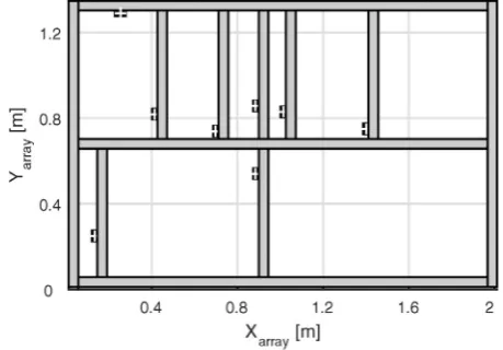
Effective directional wave gauge arrays therefore have a uniform co-array, spanning the appropriate range of magnitudes. With this criteria in mind, an 8 gauge array layout was designed for installation

on a re-configurable rig, shown inFig. 3, with the co-array and projected

in-line separations shown inFigs. 4 and 5respectively.

It is observed that the co-array of the array design is largely uniform with no duplicate vector separations, and that there is a good range of projected in-line separations for every angle of incidence. The size of

the array was chosen to ensure that there is a sufficient number of useful

separations for the frequency range of interest, taken here to be 0.2−

1.2 Hz. Analogous to the criteria proposed byGoda and Suzuki (1976)

for reflection analysis, separations are considered useful for frequency

componentiif they are between 0.05λiand 0.45λi. Asλf = 1.2 Hzis

1.08 m, andλf = 0.2 Hzis roughly 21 m, the array has been designed

so that there are a sufficient number of separations smaller than

0.49 m and larger than 1.05 m.

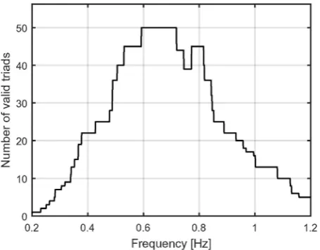
Gauges are used in groups of three to estimate wave angles, and so for a given frequency component the estimate is only assumed valid if all separations adhere to the separation criteria. The resulting number

of valid gauge triads as a function of frequency is shown inFig. 6, and

it can be seen that for the frequency components of interest there are normally multiple useful gauge triads, and hence multiple valid angle estimates.

2.3. The SPAIR method applied to the FloWave Ocean Energy Research Facility

The SPAIR method as detailed in this section uses single-summation wave generation before estimating the frequency dependent incident angles. These angles provide projected in-line separations, which are

used to perform a 2D reflection analysis for each frequency component.

Under the assumption that this frequency dependent 2D approach is Fig. 2.The single (right) and double (left) summation methods of wave generation. This

demonstrates how wave partitions made in the frequency domain are attributed unique directions (Draycott et al., 2015).

Fig. 3.Wave gauge array layout with bar positions for re-configurable rig.

valid, this enables isolation of the incident and reflected directional spectra, and time-series.

The complete method works very well for sea state validation at the FloWave Ocean Energy Research Facility. However, the combined use of all the single-summation based tools present in the SPAIR method may not always be appropriate. For example, if it is known that the wave tank produces incident waves at the correct angle then the initial

PTPD angle calculation is not required. Also if reflections are large, and

not a mirror of the incident, the reflection analysis procedure will give

unreliable results. The method limitations and sensitivity are detailed in

Section 4.1, and alternative uses of the tools are discussed inSection 4.2.

2.3.1. Input angle calculation using PTPD approach

The current methods of calculating directional spectra in tanks, such as the EMEP and BDM approaches, have been developed for ocean mea-surement and subsequently utilised for wave tank analysis. Similarly, the PTPD approach was also initially developed for use in ocean

measure-ment (Esteva, 1976; Fernandes et al., 2000). This technique has not

however made the transition to the tank environment for the routine reconstruction of directional spectra. This is likely because of the method's inability to effectively resolve directional spectra in the ocean.

The PTPD approach uses the phase difference between triads of gauges to infer the wave direction. In the ocean, and when using the double-summation method in tanks, the phase differences at a given frequency will encompass a range of wave components travelling in different directions. In practice the result is that the PTPD outputs es-sentially give a representative angle for that frequency band and cannot be used to create a full directional spectrum. When using the single-summation method of wave generation, however, there are many discrete frequency components, each of which propagates in a single direction. This should enable the method to calculate the actual directions at each sub-frequency, thereby allowing effective reconstruction of a directional spectrum when re-considering the desired, original frequency bins.

The present work uses 8 wave gauges to improve the propagation

direction estimate, as previously described byDraycott et al. (2015).

The method is implemented as follows:

1. Obtain Fourier coefficientsai,nusing an FFT for each gaugen.

Calculate amplitudesAi,nand absolute phasesΦi,n.

2. Find all 3 gauge combinations for N gauges, i.e. 8_C

3= 56.

For every triad and all frequency components:

3. Ensure relative separationsL1 , 2,L1 , 3andL2 , 3are allN0.05λi(f) and

b0.45λi(f). If so:

4. Calculate relative phasesΦ1,2andΦ1,3.

5. Calculate perceived angle,α, by the method ofEsteva (1976). The

final equations of which are shown below:

α¼ tan−1ðx1−x2ÞΦ1;3−ðx1−x3ÞΦ1;2=sgn Pð Þ

y1−y3

ð ÞΦ1;2−ðy1−y2ÞΦ1;3

=sgn Pð Þ ð3Þ

P¼½ðx1−x2Þðy1−y3Þ−ðx1−x3Þðy1−y2Þ: ð4Þ

6. Take the peak of a circular kernel density estimate over all valid triad combinations as the propagation direction for that frequency. 7. Comparisons can now be made between the desired and measured

angles, as per the single summation method. Additionally the data can be re-binned and compared with the desired directional spectrum.

The PTPD approach relies on the fact that the phase difference between gauges is a function of the frequency-dependent wave-length and their relative positions. The phase difference between

gaugenand gaugem, for a given Fourier coefficient,i, can therefore

be represented as:

Φi;nm¼ki½ðxn−xmÞcosαiþðyn−ymÞsinαi

¼ki x0i;n−x0i;m

_{: ð5Þ}

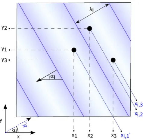
Fig. 7shows the projected in-line x-positions for frequencyi,xi,n′, as

a function of the measured wave direction,αi. Although only 3 gauges

are required to get an estimate of the wave directions it is advantageous to have multiple estimates for the propagation direction at each fre-quency. This is because measurement noise, position error and the

pres-ence, or build-up of reflections, may result in errors in individual

directional estimates.

In this work a maximum of 56 estimates are used to give a represen-tative direction for each frequency, disregarding estimates derived from triads with inappropriate separation magnitudes. A circular mean, or cir-cular median value may be used from these to estimate the true incident

direction at this frequency, however, to limit the influence from rogue

estimates a circular kernel density estimate has been used for this work. The peak of this kernel density estimate should generally represent the Fig. 5.Projected in-line wave gauge separations for a range of angles of incidence.

Fig. 6.Number of valid gauge triads (all separationsN0.05λiandb0.45λi) as a function of

incident wave direction, with estimates lying either side of the peak being

affected more strongly by reflections or position error etc.

There are 2048 kernel density estimates for each sea state, corre-sponding to the discrete frequency increments used in these tests.

Fig. 8shows some example outputs of these estimates, highlighting the requirement to have multiple estimates in some scenarios, but not

others.Fig. 8a and d highlights the advantage of using the peak of the

kernel density estimates, rather than the mean, with Fig. 8a

demonstrating this particularly well. It is clear here that using the

circu-lar mean value would have lead to a significant‘over-estimate’of the

wave direction, amounting to around 10°.

2.3.2. Calculating in-line reflections using projected gauge positions The PTPD approach used here takes advantage of the fact that the phase differences at a given frequency should be solely a function of the gauge positions and the wave propagation direction. This trait allows for the calculation of frequency dependent, in-line separations:

x0_i;n−x0_i;m¼ðxn−xmÞcosαiþðyn−ymÞsinαi: ð6Þ

The complex amplitude spectra measured at each gauge,ai,n, along

with these assumed separations then allow a reflection analysis

proce-dure to take place. The process in doing this essentially treats each frequency component as a uni-direction problem.

Typical uni-directional reflection analysis can be achieved with a

small number of gauges, as demonstrated byGoda and Suzuki (1976)

for 2 gauges, andMansard and Funke (1980), using a least-squares

approach with 3 gauges. These methods require the gauge separations to be within a small range to give useful estimates. In this multi-directional work the effective in-line separations are highly variable, and as such require more gauges to ensure useful spacings are available.

Zelt and Skjelbreia (1992)present an extension to the Mansard & Funke method, formulating a weighted least-square approach to

estimating incident and reflected wavefields for any number of gauges.

This approach is used in this work with some slight modification. The

three modifications made are as follows:

1. x-Values are now frequency dependent in-line x-positions, based on

the calculated_αvalues.

2. Absolute phases are used rather than phase difference to gauge 1.

This eventually allows reconstruction of total, incident, and reflected

time-series, and also direct use of the isolated Fourier coefficients.

3. As a weighting function the goodness function presented inZelt and

Skjelbreia (1992)is used in conjunction with the coherence spectra between gauges (dot product). This should enable spacing consider-ations (goodness function) to be considered in conjunction with a measure of the consistency of the phase differences between gauges. In the results presented here this has made little improvement

(b2%). If, however there are particularly noisy signals, or if complex

reflections build up throughout a test this may prove more useful.

The coherence spectra were calculated using the in-built mscohere MATLAB function.

Thefinal modified equations used to calculate the complex incident

and reflected Fourier coefficients,aincandarefare shown below:

ainc;i¼

XN

n¼1

Ci;nai;n ð7Þ

aref;i¼

XN

n¼1

Ci;nai;n ð8Þ

whereai,nis themeasuredFourier coefficients with absolute phase

(rather than with phases relative to gauge 1), and

Ci;n¼

2iWi;n

D XN

m¼1

Wi;msinΔΦi;nmeiΦi;m ð9Þ

D¼4X N

n¼1

X

mbn

Wi;nWi;msinΔΦi;nm 2

ð10Þ

Fig. 7.Example projected x values for a single frequency component and its associated propagation direction.

where:

ΔΦi;nm¼ki½ðxn−xmÞcosαiþðyn−ymÞsinαi ¼ki x0i;n−x0i;m

ð11Þ

Φi;m¼kix0i;m: ð12Þ

Wi,nis the weighting function for gauge n and frequency i. SeeZelt

and Skjelbreia (1992)for the goodness function, andMandel and Wolf (1976)for information on coherence spectra.

These equations allow the incident and reflected amplitude spectra

to be resolved for single-summation generated directional spectrum.

The incident and reflected wave energy density spectra can now be

calculated as:

Sinc;i¼ ainc;i

2

2δf ð13Þ

Sref;i¼ aref;i

2

2δf : ð14Þ

The frequency-dependent reflection coefficient,Kr,i, can also be

readily calculated as:

Kr;i¼ aref;i

ainc;i : ð

15Þ

2.3.3. Calculating the updated incident, and the reflected directional spectrum

Knowledge of the incident and reflected wave frequency spectrum

does not allow for an update to be made to the incident directional

spectrum directly. The re_flections present in the tank cause gauge

dependent amplitude and phase deviations. The nature of the PTPD approach means that these can manifest themselves as a directional distribution error, rather than being isolated. This requires the incident propagation directions to be recalculated, using the already isolated

incident Fourier coefficients.

In order tofix the measured incident directional spectrum the isolated

incident Fourier coefficients can be re-processed using the PTPD

approach. This requires the phases for the base Fourier coefficients,

ainc,i, at [0,0], to be shifted to the in-line apparent gauge positions.

This is done noting that:

ai;n¼ainc;ie−iΦi;nþaref;ieiΦi;n: ð16Þ

This de_fines the incident, position shifted Fourier coef_ficients as:

ainc;i;n¼ainc;ie−iΦi;n¼ainc;ie−i kix

0

i;n

: ð17Þ

These Fourier coefficients can now be used directly with the PTPD approach, enabling an estimate of the incident directional spectrum to

be made with an attempt to remove the artificial amplitude and phase

deviations. The reflected directional spectrum can be calculated similarly,

or more easily through knowledge of the reflection coefficients. In

addition to this, the incident and reflected time series at the gauge

posi-tions can be estimated through an IFFT.

The nature of this combined approach means that incident and

reflected spectra can be separated over all directions without requiring

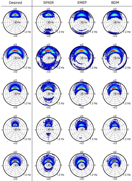
prior knowledge of the input angular range. Neither the BDM or EMEP Fig. 10.Example SPAIR reconstructed directional spectra outputs. Energy density [m2

Fig. 11.Example time series outputs for the example spectra shown inFigs. 9 and 10. Theoretical time series as well as measured are shown, in addition to the isolated incident and reflected components for a range of gauges. Sea state 1, gauge 1; sea state 2, gauge 2 etc.

approaches are capable of achieving this, and even with a de_fined input range are shown to exhibit much larger uncertainties.

3. Results

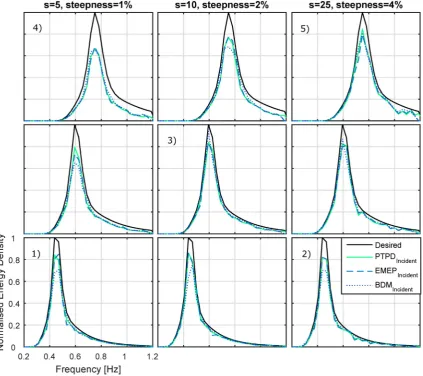
3.1. Frequency spectra

Example incident frequency spectra are shown inFig. 9. These

provide results for a range of sea states covering both the highest and

lowest re_flection conditions, as shown inFig. 12. There is an apparent

tendency to under-produce waves, particularly at the spectral peak, and whilst being more pronounced for sea states with higher peak

frequency, and inherently higher re_flections, it is prevalent throughout.

In general the deviation is much lower for sea states with lower peak frequency, suggesting that, as expected, the tank's generating and absorbing effectiveness reduces above a certain frequency threshold. To demonstrate that this deviation isn't a function of the method, and

to allow comparisons to be made inSection 3.5.1, the frequency spectra

outputs for the BDM and EMEP approaches are also been shown. This deviation, despite being consistent, is also easy to rectify. Linear frequency dependent correction factors can be applied as a function of the deviation between the target amplitude spectrum and the isolated incident spectrum. These have proved to be effective in previous tests,

bringing down the relative deviation to 1−2%. As the current tests are

focussed on directional distribution and re_flection calculation it was

not deemed necessary to apply them for this purpose.

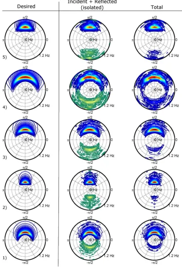
3.2. Incident and reflected directional spectra

Directional spectra relating to the numbered frequency spectra in

Fig. 9are shown inFig 10, ensuring the extremes of the test programme are still included. The majority of sea states shows good agreement between the input and measured spectra. The difference between the measured incident spectrum from the desired input is generally low, with the exception of sea state 4. Viewing the colour-scale-separated

spectra (middle column ofFig. 10) it is apparent that the reflected

spectrum has been effectively isolated, generally mirroring the form of the incident distribution.

It is apparent that example sea state 4 demonstrates much larger

deviations than the others.Fig. 9highlights that this is largely due to

significant under-generation, whilst inFig. 12it is observed that the

reflection coefficient is also very high. This re-iterates thefindings that

high frequency, low amplitude waves are generated, and absorbed less effectively, especially when combined with high directional spreading.

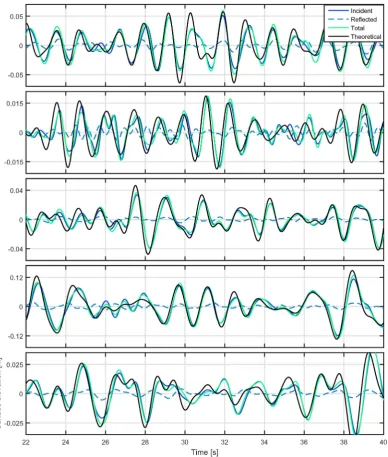
3.3. Time series

Fig. 11shows the example time series outputs for the spectra in

Fig. 10. An IFFT of the complex input amplitude spectra enables the Fig. 13.Mean frequency dependent reflection coefficients for each peak frequency averaged over directional spreading, separated by steepness. Normalised wave spectra overlaid to aid explanation of overall reflection coefficients (Fig. 12).

theoretical time series to be computed using linear wave theory, before

being compared to the actual measurements. As shown inSection 2.3.3,

the presented method also allows for the separation of incident and

reflected time series in the tank domain, and as such these have been

computed at the gauge locations for comparison.

The measured time series outputs show reasonably good agreement with the theoretical time series calculated using linear wave theory. The

removal of the reflected components generally provides a closer match,

however, this is not always the case. The isolation of what is unaccounted

reflections from non-linear behaviour appears difficult. As expected from

Fig. 15.Comparison of example directional spectrum outputs from SPAIR, EMEP and BDM approaches. Energy density [m2

the spectral analysis, example sea state 4 shows the largest deviations,

and also the largest relative reflected components.

3.4. Reflection analysis

The output of the directional reflection analysis for the 3 × 3 ×3 test

matrix is shown inFig. 12. Reflections in the FloWave facility are

primarily related to the absorption characteristics of the force-feedback wavemakers, and as such are both frequency and amplitude dependent.

This is demonstrated inFig. 12where it can be clearly observed

that increasing peak frequency, or decreasing wave steepness,

causes an increase in the overall wave re_flection coef_ficient. This

frequency dependency can be attributed to the paddle characteristics,

as well as absorption control scheme, as explored inGyongy et al.

(2014). The reduced sensitivity of the force-feedback mechanism to low wave forces appears to drive the decreased absorption effectiveness for small, low steepness waves.

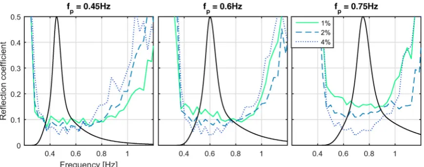
Fig. 13shows the mean frequency dependent reflection coefficients for each peak frequency used, averaged over directional spreading. This enables a more detailed frequency dependent exploration of the

reflection coefficients, and offers further explanation to the results

shown inFig. 12.

3.5. Method performance

3.5.1. Comparison to other methods

In order to assess combined sea state and method performance, the Normalised Total Difference (NTD) between target and measured

spectra can be assessed, defined as:

For directional spectra:

NTDE¼

XNf p¼1

XNθ

q¼1Ei;pq−Em;pq

XNf p¼1

XNθ q¼1Ei;pq

: ð18Þ

For frequency spectra:

NTDS¼

XNf

p¼1Si;p−Sm;p

XNf p¼1Si;p

: ð19Þ

NTDEprovides assessment of the total deviation from target spectra,

which includes:

• frequency spectrum error,NTDS

• directional distribution error,NTDD

• method reconstruction error,NTDM

• miscellaneous (other) error,NTDOe.g. noise, position error.

Ideally the method reconstruction error,NTDM, would be assessed to

gauge method performance. It is not possible, however, to isolate this as

the true directional distribution error is not known.Fig. 9shows that the

deviation from target frequency spectra,NTDS, is mostly tank dependent

and not a function of the methodology. For these reasons to assess

meth-od performance,NTDE–NTDShas been used, noting that it incorporates

the method reconstruction error, along with the directional distribution error. As the true distribution error is constant this should allow effec-tive comparisons to be made between methods.

Fig. 14shows this comparison for the calculated incident spectra

(using afixed input range of 0–180° for BDM and EMEP methods)

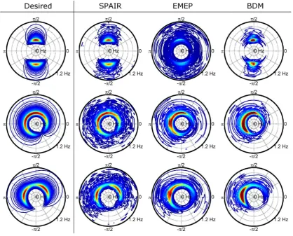
Fig. 16.Complex directional spectra outputs (total) for SPAIR, BDM and EMEP approaches. Energy density [m2

over the initial 3 × 3 × 3 test plan. The SPAIR approach consistently per-forms better, with a mean NTD of 5.93%, compared with 16.1 and 21.7% for the EMEP and BDM approaches respectively.

Example directional spectrum outputs from these methods are

shown inFig. 15, for the same sea states as shown inFig. 10. It can be

seen that neither the EMEP or BDM approaches consistentlyfit a DSF

that incorporates reflected components. The EMEP approach appears to

incorporate some re_flected energy content, but the distribution seems

incorrect, likely constrained by the inherent frequency-dependent

‘curve-fitting’process.

Visually all of the methods perform reasonably well in terms of

characterising the incident wavefield, with the SPAIR approach

demon-strating the best performance, as shown inFig. 14. This is also apparent

through visual observation, as the high energy components of the incident distribution match up very well with that of the desired. At low energy levels, however, the distribution does appear to be

ill-defined, a function of the discretised nature of the solution, and the

low energy densities present at these frequencies.

3.5.2. Performance with complex spectra

The complex spectra de_fined inTable 3have no de_fined incident and

reflected range and as such the EMEP and BDM approaches cannot

resolve the reflected components.Fig. 16shows the total reconstructed

wavefield using the three methodologies. It is clear that the EMEP and

BDM approaches generally fail to capture the multi-modal and highly spread nature of the input sea states, other than perhaps the BDM approach reconstruction of sea state 3.

The SPAIR approach enables a much more effective characterisation

of the input conditions, as demonstrated inFig. 16andTable 4. The

reflected spectrum and coefficients can also be calculated as no input

angular range is required, with the result that the incident and reflected

spectra can apparently overlap. The reflected spectra are shown in

Fig. 17, and the total reflection calculated coefficients were found to be 8.36, 8.61 and 8.13% respectively.

Each of the unusual spectra have peak frequencies of between

0.45 Hz and 0.5 Hz, around 2–3% steepness, and large spreading. Despite

having vastly different spectral forms they have near identical reflection

coef_ficients, consistent with the results shown inFig. 12. This supports

previousfindings that peak frequency and steepness are the main

parameters to which absorption effectiveness is sensitive to, along with some sensitivity to directional spreading.

4. Discussion

4.1. Method limitations and sensitivity

4.1.1. Effect of in-line reflection level

The presence of in-line reflections alter the phases and phase

differences measured at the gauges, and hence causes an apparent

angle estimation error through Eq.(3). The effect of this can be

under-stood by looking at the resulting Fourier coef_ficients in the presence of

such reflections.

Table 4

Directional distribution error,NTDE–NTDS, for complex spectra.

NTDE–NTDS Sea state 1 Sea state 2 Sea state 3

SPAIR 0.153 0.127 0.054

EMEP 0.340 0.227 0.454

BDM 0.414 0.344 0.322

Fig. 17.Incident and reflected directional spectrum outputs for complex spectra defined inTable 3. Energy density [m2

Surface elevations in the presence of in-line reflections, at [x,y], can be modelled as:

ηðx;y;tÞ ¼X

N

n¼1

Ainc;icoski xcosαinc;iþysinαinc;i

þΦinc;iþωit

þKr;iAinc;icos−kixcosαinc;iþysinαinc;i

þΦinc;iþΦref;iþωitÞ:

ð20_Þ

Definingki,xy=ki(xncosαinc,i+ynsinαinc,i), andkr,i=Kr,ieiΦref,i, the

resulting Fourier coefficients at gauge n can be expressed as:

ai;n¼ainc;ieiki;xyþainc;ikr;ie−iki;xy

¼ainc;icoski;xyþisinki;xyþainc;ikr;icoski;xy−isinki;xy

¼ainc;i 1−kr;i

isinki;xy

þainc;i 1þkr;i

cos ki;xy

:

ð21Þ

The expected phase at gauge n is therefore:

Φn;i¼atan

tanki;xy1−kr;i

1þkr;i

" #

: ð22Þ

Apparent angle for each gauge triad is calculated using:

αapparent;i¼tan−1 x1−x2

ð ÞΦi;13−ðx1−x3ÞΦi;12

=sgn Pð Þ

y1−y3

ð ÞΦi;12−ðy1−y2ÞΦi;13

=sgn Pð Þ ð23Þ

where:

Φi;mn¼Φm;i−Φn;i: ð24Þ

From Eq.(22)it can be seen that phases and phase differences at the

gauge locations are heavily influenced by the magnitude of the reflection

coefficient,Kr,i. However the extent with which this alters the resulting

angle estimation depends on the relative change inΦi,13toΦi,12, which

is a function of the angle relative to the triad orientation, along with the magnitude of the separations relative to the wavelength.

Fig. 18.Effect of in-line reflection coefficient, wave angle and relative separation magnitude on apparent angle calculation.

Fig. 19.Uni-directional spectrum for numerical sensitivity analysis.Hm0= 0.2. For the

simulations, an incident angle ofθ=22.5°has been used.

Fig. 18shows the expected angular error for a single equilateral

gauge triad as a function of the reflection coefficient, incident angle

and relative separation magnitude.Krvalues between 0 to 10 have

been used to assess whether the PTPD method presented identifies

the‘reflected’component as the incident direction if KrN1. From

Fig. 18it is apparent that the method doesfind the correct‘dominant’

angle whenKrN1.

It is clear that if gauge separations are small then the angle calculation

is relatively unaffected by the level of reflection. Practically, however, if

gauge separations aretoosmall relative to all frequency components,

position error and noise will alter the measured phases more greatly and hence cause increased errors in the apparent angle estimates.

As expected, when reflection levels are low the angular estimates

are also largely unaffected. When reflections are large, however, the

incident angle relative to the gauge triad orientation becomes

impor-tant, highly influencing the values of individual angle estimates. Overall

the effect of these poor individual estimates can be minimised by designing a wave gauge array so that for each frequency (wavelength) there is a uniform co-array distribution of valid separations. If this is the case, using all of the estimates, the kernel density estimate approach

discussed inSection 2.3.1should be able to provide the correct incident

angle.

To assess how the kernel density approach with the array layout

shown inFig. 3deals with different levels of reflection, a numerical

simulation has been carried out, using a uni-directional broad-banded

spectrum with frequency independent in-line re_flections. This spectrum

has been used as it covers the operational frequency range of the tank

(0.2→1.2 Hz), whilst enabling easy analysis and viewing of results.

This spectrum is shown inFig. 19and is also used for the sensitivity

analysis shown inSection 4.1.2.

Fig. 20shows the angular error resulting from the simulation. It is clear that the combination of the array and method used performs

very well for frequencies up to 0.95 Hz, regardless of the level of refl

ec-tion. The error shown is purely a function of the number of bins used for

the kernel density estimate (250). When reflection is relatively low

(Krb0.5) there is also no perceived error in the angle estimate, at any

frequency. This shows that the array-method combination performs

very well in general, especially for the level of reflection present in the

(empty) FloWave basin. Once this initial angle is effectively identi_fied

the subsequent in-line reflection analysis will then be correct, which

can be seen inFig. 23when the oblique reflection angle is 0°.

Errors arise from 0.95 Hz onwards when the reflection coefficient is

over 0.5, due to the smaller number of valid gauge triads (seeFig. 6).

This means that poor individual estimates have a greater effect on the

final angle calculation, a result of the combined effect of larger reflections,

triad orientation and large relative separations. Individual estimates for

1 Hz with a range of reflection scenarios are illustrated inFig. 21,

demon-strating how individual estimates are affected by reflection levels and

how the kernel density estimate mitigates the effect of these on the

final angle values.

Where large reflections and high wave frequencies are present it

may be necessary to use an array with additional gauges placed closer together. This would ensure that there are enough gauge triads with

Fig. 22.Effect of reflection level and angle on the mean apparent angle (over all frequencies).

separations less than 0.45λi, thus improving the high frequency

esti-mates. For the levels of reflection present in the empty tank the current

array layout should be suitable for identifying the correct incident angle regardless of frequency. That is, under the assumption that position

error and noise are negligible, and more importantly, that reflections

can be assumed to be in-line. This will be discussed inSection 4.1.2.

4.1.2. Effect of reflection angle and curvature

4.1.2.1. Oblique reflections.InSection 4.1.1it was found that the level of

in-line reflection does not greatly affect the correct identification of

the incident angle when using the current implementation of the meth-od in combination with the wave gauge array. This additionally enables

a correct in-line reflection analysis to take place. If, however, the refl

ec-tions are not in-line then this is no longer the case.

Introducing a change in reflected angle,Δαref,i, the surface elevations

become:

ηðx;y;tÞ ¼XN

n¼1

Ainc;icoskixcosαinc;iþysinαinc;iþΦinc;iþwit

þKr;iAinc;icos−kixcosαinc;iþΔαref;i

þysinαinc;iþΔαref;i

Þ þΦinc;iþΦref;iþwitÞ:

ð25Þ

Definingki,α,xy=ki(xcos (αinc,i+Δαref,i) +ysin (αinc,i+Δαref,i), the

resulting phases can be shown to be:

Φn;i¼atan

ainc;isinki;xy

−kr;iainc;isinki;α;xy

ainc;icos ki;xy

þkr;iainc;icoski;α;xy

" #

: ð26Þ

It can be seen from Eq.(26)that the phase differences will be altered

by the magnitude of_Δαref,iin addition to the level of re_flection and array

layout. The difference here compared with the in-line reflection analysis,

Eq.(22), is that when the angles are calculated using Eq.(3), the

‘direction’of the angular error is now no longer solely a function of

the triad layout, and as such does not‘average’out over multiple

esti-mates. All angle estimates now contain a consistent error as a function ofΔαref,i.

Using the spectrum shown inFig. 19, and simulating the oblique

reflections over the array we can observe this consistent shift in angle

estimate, shown inFig. 22. This shows that if there are sizeable refl

ec-tions with even a small re_flection angle then the PTPD approach cannot

be used to effectively identify the incident angle.

As discussed inSection 4.2.2it is not always necessary to estimate

the incident angle. To further assess how oblique re_flections affect the

isolation of incident and reflected spectra the incident angles are

assumed to be known.Fig. 23shows how the level, and angle of refl

ec-tion, affect the isolation of incident and reflected spectra. As expected,

this shows that it is not appropriate to use in-line reflection analysis

when the reflections are oblique relative to the incident. This is because

the phase differences are no longer a function of the‘in-line’gauge

separations assumed in the analysis. It may however be suggested

that results are still somewhat useful if the reflection angle is low,

perhaps less than 20°.

4.1.2.2. Curved reflections.When reflections are curved or directionally spread, there will be larger variation in the individual angle estimates generated using the gauge triad combinations. If the mean direction of the curved waves is not opposite the incident, then similar behaviour is to be expected to the oblique wave analysis, but with additional scatter. If, however the mean direction of the curved waves opposes

the incident, then the correct incident angle can be identi_fied with an

appropriate array, and a meaningful representative in-line reflection

analysis procedure can take place. This is the case at FloWave. The circular wave basin at FloWave ensures that the mean direction

of reflected components opposes the incident direction. The circular

shape also means that the reflected components are curved, as a

func-tion of the wave basin geometry and the angular dependency of the tank transfer function.

Reflected wave curvature has been analysed through the spatial

variation of measured wave heights. As it is known that the incident waves are long crested and uniform, the variation in wave height is

solely a function of the curved reflected components interacting with

the incident waves. An example‘spatial map’is shown inFig. 24for

0.45 Hz regular waves, noting that from further tests the curvature of

these reflections appears to be independent of wave frequency. Over

the small array area (1 m2_{) the assumption that curvature is negligible}

for the purpose of reflection analysis seems appropriate.

Fig. 24.Spatial map of wave height variation for 0.45 Hz regular waves (2% steepness). Shows reflected wave curvature over the tank operational area (roughly equal tofloor area).

Fig. 25.Effect of mean direction on perceived sea state performance. Maximum and minimum values of the test programme shown in dashed lines.

Fig. 26.Effect of mean direction on perceived reflection coefficient. Maximum and minimum values of the test programme shown in dashed lines.

The results presented here clearly shows that for the level of refl ec-tion and curvature present, the incident angle can be effectively

identi-fied using PTPD approach with the wave gauge array shown inFig. 3.

Once these are identified the co-array uniformity and least squares

approach of the reflection analysis should ensure that the

representa-tive in-line reflection coefficients are valid despite these small levels of

curvature. This should give a very good estimate of the incident and

reflected spectra, and time-series, over the array area. This approach

means that sea states can be effectively characterised in a particular location (generally in the tank centre), prior to use in a test programme with a model installed.

FromFig. 24, it is apparent that the effective reflection coefficient is not constant, and in fact varies in the in-line direction due to circular

focussing effects. As a result of this, and the reflected wave curvature,

it is clear that the reflected directional spectrum is spatially variable.

This means that although the isolation of incident and re_flected spectra,

and time-series over the array area gives reliable results, using this 2D approach to extrapolate far from the measurement area will not be accurate. However, through knowledge of the wave curvature and

in-line dependency of the reflection coefficient, it should be possible

to alter the energy density and angles in the reflected spectrum, and

amplitudes and phases in the time-series reconstructions to provide reasonable estimates over the tank area, if desired.

4.1.3. In_fluence of mean direction

The wave generating capability at FloWave is designed to be directionally independent, meaning that any change in mean wave

propagation direction should not in_fluence the sea state performance.

Any perceived changes should therefore be attributed to the array layout, and the method itself.

Figs. 25 and 26show the perceived reflection coefficient and direc-tional NTD variation incurred by varying mean direction for a single

sea state. The sea state used is detailed inTable 2. It can be seen in

Fig. 26that when altering the mean direction, the perceived reflections

also vary. This is coupled with variation in the perceived directional distribution error.

Without the presence of re_flections, noise, or position error, there

would be no error in the measured propagation directions, and hence no discrepancy in the directional distribution. Of these factors, the

presence of reflections is probably the largest contributor in most

circumstances. It is observed to have a consistent effect on both the relative phases, and the amplitudes at the gauge locations.

As the mean direction changes, the array layout plays an important

role, as the relative reflection and error-influenced phase differences

are dependent on the projected in-line separations. These deviations cause differences in the perceived angles and hence incur a varied and largely unpredictable directional distribution error. A portion of the perceived directional deviation for any sea state is therefore a complex

function of the induced phase errors (mostly reflection based), and

the array layout.

4.1.4. Influence of primary sea state parameters on performance

Analysing the variation in NTD, it is difficult to assess what

propor-tion of this difference is the result of actual sea state deviapropor-tion, and what can be attributed to the array-methodology effectiveness under

various conditions. This was one of the reasons for usingNTDE–NTDS

Fig. 29.Influence the number of gauges has on the directional distribution error, along with the standard deviation of this error.

Table 5

Number of gauge combinations available.

Number of gauges Number of combinations

3 56

4 70

5 56

6 28

7 8

8 1

inSection 3.5.1, removing the frequency spectrum deviation, and focus-sing on the directional distribution reconstruction.

The total deviation,NTDE, and the frequency spectrum deviation,

NTDS, essentially show the same dependencies as the reflection coeffi

-cient, shown inFig. 12. It appears that higher peak frequency sea states

with low steepness incur both greater reflections, and larger deviations

in the incident spectrum simultaneously. The correlation between NTD

and reflection coefficient can be seen inFig. 27.

The directional deviation metric,NTDE–NTDS, appears not to have

a predictable correlation to reflection coefficient, as discussed in

Section 4.1.3.Fig. 28shows the relationship between the directional distribution component, and the primary sea state parameters. The only apparent relationship appears to be a reduced NTD when

spreading is lower (sis higher). This is potentially expected as the

only two parameters affecting directionality are spreading and mean

direction, of which, mean direction has been fixed for the main

3 × 3 × 3 test matrix.

4.1.5. Influence of number of gauges

As discussed inSection 4.1.3increasing the number of gauges, if

po-sitioned correctly, should reduce the sensitivity to wave directionality. In general, additional gauges should give rise to improved estimates

and reduced directional discrepancy between target and measured spectra. To explore the effect of the number of gauges all gauge combi-nations with 3 or more gauges have been assessed under an individual

sea state (Table 2,θ¼36). The number of combinations for a desired

number of gauges is shown inTable 5, whilst the mean directional

devi-ation and the standard devidevi-ation of this between array layouts is shown inFig. 29. As expected, the mean directional deviation reduces with the use of more gauges. The standard deviation of the directional deviation is also shown, describing the expected variation in performance when using different sets of gauges.

Increasing the number of gauges will further reduce both the direc-tional deviation and the variation between hypothetical gauge subsets. As the gauge combination choice is analogous to an effective change in wave direction, this will further reduce the sensitivity of an array to direction, thus improving the reliability of the estimates under a variety of wave conditions.

4.2. Alternative applications

4.2.1. No reflection analysis: PTPD approach only

As demonstrated inDraycott et al. (2015), using the PTPD approach

to reconstruct directional spectra at FloWave works effectively without

the addition of reflection analysis. This works particularly well at the

FloWave facility (or other circular wave basins with active absorption)

as the reflections are low, and can be approximated as in-line. It should

also be effective for tanks with different geometry, providing re_flections

are relatively low, and the reflection angle isn't very large (seeFig. 22). If

this is the case then the incident directions should be effectively

identi-fied, and a more accurate representation of the incident directional

spectrum should be attained than when using the EMEP or BDM approaches.

4.2.2. No angle calculation: assumed incident angles

Sections 4.1.1 and 4.1.2show that under certain conditions the

pres-ence of reflections can introduce errors in the incident angle calculation.

This, consequently, means that the projected in-line reflection analysis

is done at a slightly incorrect angle thus meaning that the reflection

coefficients themselves will be incorrectly calculated, along with the

incident and re_flected spectra. If it can be assumed that the incident

wave propagation angles are known, and precisely produced, then

reflection coefficients can be calculated more accurately, whilst giving

a better representation of the re_flected wave_field.

Fig. 30shows the relative time lag between gauges mounted perpendicular to the expected wave propagation direction, for a variety of regular waves with different frequencies. Sampled at 128 Hz, it can be seen that the phase lags are all less than 1 time step. This shows that the

Fig. 31.Influence assuming the incident direction has on the reflection coefficient calculation.

desired angle is precisely produced with negligible curvature, at least from ±8 m from the tank centre. This analysis was done on only the

first few regular waves (to avoid re_flections), however it is probably a

good assumption that the generation capability is not greatly affected by either simultaneous absorption or the generation of multi-directional sea states. Therefore the incident angles can be assumed correct at FloWave.

The resulting overall reflection coefficients when the assumed input

angles are used are shown inFig. 31. It is apparent that when the refl

ec-tions are larger, the greater the error in the computed reflection coeffi

-cient, highlighting this‘feedback loop’problem. In general however, the

reflection coefficients agree very well and it is clear that the computations

where angle isn't assumed will provide adequate practical reflection

estimations in the majority of cases.

4.3. Further work

Further work aims to include an extension to handle oblique refl

ec-tions, potentially using a procedure similar toWang et al. (2008). This

ex-tension, along with an understanding of the geometry in question would

enable directional reflections to be calculated accurately for other objects

such as rectangular tanks, or indeed other structures and devices. The idea

of enabling of reflections to be resolved using double summation

ap-proaches, or as curved components will also be explored, enabling the

reflected components to have a spread at each frequency.

5. Conclusions

The directional characteristics of sea states are often relevant to ocean and coastal engineering problems. The capability of wave basins to produce more complex multidirectional sea states has expanded in recent years, with many facilities now having wavemakers along multi-ple boundaries, or in the case of circular tanks, around the entire circum-ference. The ability to generate more complex spectra, including those with extreme spreading and multi-modality, brings about challenges in validating and calibrating these sea states and highlights the limita-tions in the established measurement techniques. To this end the SPAIR method has been developed. A single-summation method of wave generation has been used to generate a range of directional sea state conditions in a circular wave tank, FloWave. A phase-time-path difference approach has then been used to calculate wave propagation

angles, before frequency-dependent in-line reflection analysis is

performed.

This method, SPAIR, has proved to be highly effective in the measurement of multidirectional sea states within a circular wave

tank, providing both incident and reflected directional spectra, and

reconstructed time-series. The method has been demonstrated with both standard parametric and more complex multi-modal and extremely spread seas. When this single-summation method of wave generation is used, the PTPD-based reconstruction method has shown to be more effective at validating directional sea states

than either the EMEP or BDM approaches, reducing the mean apparent directional deviation from 16.1% (EMEP), and 21.7% (BDM), down to 5.93%.

Sensitivity analysis shows that method itself, in combination with the

wave gauge array, has very low sensitivity the level of in-line reflection,

particularly for the range expected at the FloWave facility. However,

high sensitivity is displayed to the presence of oblique reflections,

something which future work aims to deal with.

Acknowledgements

The authors would like to thank the Energy Technology Institute and the Research Council UK Energy Programme for funding this research as part of the IDCORE programme (EP/J500847/1). In addition we would like to thank the UK Engineering and Physical Science Research Council for funding towards the creation of the FloWave Ocean Energy Research Facility (EP/I02932X/1).

References

Benoit, M.P., Frigaard, P., Schaffer, H.A., 1997.Analysing multidirectional wave spectra: a tentative classification of available methods. Assoc. Hydraulic Res. Seminar: Multidirec-tional Waves.

Draycott, S., Davey, T., Ingram, D.M., Lawrence, J., Day, A., Johanning, L., 2015.Using a Phase-Time-Path-Difference Approach to measure directional wave spectra in FloWave. EWTEC Conference Proceedings.

Esteva, D., 1976.Wave direction computations with three gage arrays. Coastal Engineering Proceedings.

Fernandes, A.A., Sarma, Y.V.B., Menon, H.B., 2000.Directional spectrum of ocean waves from array measurements using phase/time/path difference methods. Ocean Eng. 27 (4), 345–363.

Goda, Y., Suzuki, T., 1976.Estimation of incident and reflected waves in random wave experiments. Coastal Engineering Proceedings, pp. 828–845.

Gyongy, I., Bruce, T., Bryden, I., 2014.Numerical analysis of force-feedback control in a circular tank. Appl. Ocean Res. 47, 329–343 (August).

Hashimoto, N., Konbune, K., 1988.Directional spectrum estimation from a Bayesian approach. Coastal Engineering Proceedings, pp. 62–76.

Hashimoto, N., Nagai, T., Asai, T., 1994.Extension of the maximum entropy principle method for directional wave spectrum estimation. Coastal Engineering Proceedings, pp. 232–246.

Haubrich, R.A., 1968.Array Des. 58 (3), 977–991.

Ingram, D., Wallace, R., Robinson, A., Bryden, I., 2014.The design and commissioning of thefirst, circular, combined current and wave test basin. Flow3d.com.

Krogstad, H.E., 1988.Maximum likelihood estimation of ocean wave spectra from general arrays of wave gauges. Modeling, Identification and Control.

Mandel, L., Wolf, E., 1976.Spectral coherence and the concept of cross-spectral purity. J. Opt. Soc. Am. 66 (6), 529.

Mansard, E.P.D., Funke, E.R., 1980.The measurement of incident and reflected spectra using a least squares method. Coastal Engineering Proceedings, pp. 154–172.

Miles, M.D., Funke, E.R., 1989.A Comparison of Methods for Synthesis of Directional Seas.

Pascal, R.C.R., 2012.Quantification of the Influence of Directional Sea State Parameters Over the Performances of Wave Energy Converters.

Wang, S.K., Hsu, T.W., Weng, W.K., Ou, S.H., 2008.A three-point method for estimating wave reflection of obliquely incident waves over a sloping bottom. Coast. Eng. 55 (2), 125–138 (February).