MoL 2017 22: Turing Learning with Nash Memory

Turing Learning with

Nash Memory

Machine Learning, Game Theory and Robotics

Shuai Wang

Master of Science Thesis

University of Amsterdam

Local Supervisor: Dr. Leen Torenvliet (University of Amsterdam, NL)

Co-Supervisor: Dr. Frans Oliehoek (University of Liverpool, UK)

Turing Learning is a method for the reverse engineering of agent behaviors. This approach was inspired by the Turing test where a machine can pass if its behaviour is indistinguishable from that of a human. Nash memory is a memory mechanism for coevolution. It guarantees monotonicity in convergence. This thesis explores the integration of such memory mechanism with Turing Learning for faster learning of agent behaviors. We employ the Enki robot simulation platform and learns the aggregation behavior of epuck robots. Our experiments indicate that using Nash memory can reduce the computation time by 35.4% and results in faster convergence for the aggregation game. In addition, we presentTuringLearner, the first Turing Learning platform.

Keywords: Turing Learning, Nash Memory, Game Theory, Multi-agent System.

COMMITTEEMEMBER: DR. KATRINSCHULZ(CHAIR) PROF. DR. FRANK VANHARMELEN DR. PETER VANEMDEBOAS DR. PETERBLOEM

YFKEDULEK MSC

MASTERTHESIS, UNIVERSITY OFAMSTERDAM

Contents

1

2

2.1 Introduction to Game Theory 9 2.1.1 Players and Games . . . 9

2.1.2 Strategies and Equilibria . . . 10

2.2 Computing Nash Equilibria 11 2.2.1 Introduction to Linear Programming . . . 11

2.2.2 Game Solving with LP . . . 12

2.2.3 Asymmetric Games . . . 13

2.2.4 Bimatrix Games . . . 14

2.3 Neural Network 14 2.3.1 Introduction to Neural Network . . . 14

2.3.2 Elman Neural Network . . . 15

2.4 Introduction to Evolutionary Computing 16 2.4.1 Evolution . . . 16

2.4.2 Evolutionary Computing . . . 16

3

3.1 Introduction to Coevolutionary Computation 19 3.1.1 Coevolution and Coevolutionary Computation . . . 19

3.1.2 Coevolutionary Architectures . . . 20

3.3 The PNG and RNG Game 23

3.4 Turing Learning 25

3.4.1 Inspiration and Background . . . 25

3.4.2 Turing Learning Basics . . . 26

3.4.3 Architecture and System . . . 27

3.5 Aggregation Game 28

4

4.1 Nash Memory 31 4.1.1 Memory Methods and Solution Concepts . . . 31

4.1.2 Introduction to Nash Memory . . . 32

4.1.3 The Operation of Nash Memory . . . 33

4.1.4 Nash Memory in Application . . . 35

4.2 Parallel Nash Memory 35 4.3 Universal Nash Memory 37 4.3.1 Introduction to Universal Nash Memory . . . 37

4.3.2 Towards Universal Nash Memory in Application . . . 38

4.4 Evaluation 39 4.4.1 ING Game . . . 40

5

5.1 TuringLearner: Design and Modelling 43 5.1.1 Strategies, Players and Games . . . 44

5.1.2 Turing Learning and Aggregation Game . . . 46

5.2 Implementation 47 5.3 Evaluation 50 5.3.1 The PNG and RNG Game . . . 50

5.3.2 Aggregation Game . . . 53

6

6.1 Discussion and Future Work 67 6.1.1 Games and Solvers . . . 67

6.1.2 Architecture, Types and Metaprogramming . . . 68

6.1.3 Models and Classifiers . . . 69

6.2 Conclusion 70 6.3 Acknowledgement 70

A

5

A.1.2 A simple example: a robot and a world . . . 72 A.1.3 Viewer . . . 73 A.1.4 Object . . . 76

A.2 GNU Scientific Library (GSL) 77

A.3 Solve the Rock-Paper-Scissors Game with PuLP 77

1. Introduction

Turing Learning is a method for the reverse engineering of agent behaviors [20]. This approach was inspired by the Turing test where a machine can pass if its behaviour is indistinguishable from that of human. Here we consider a human as a natural/real agent and a machine as an artificial agent/replica. The behaviour of each agent follows their internal model respectively. In this test, an examiner is to tell two kinds of agents apart. The Turing Learning method follows a co-evolutionary approach where each iteration consists of many experiments like that of Turing test. On the one hand, this co-evolutionary approach optimizes internal models that lead to behavior similar as that of the individuals under investigation. On the other hand, classifiers evolve to be more sensitive to the difference. Each iteration of Turing Learning can be considered a game between models and classifiers with the result of experiments as payoff. This co-evolutionary approach has been reported to have better accuracy than classical methods with predefined metrics [20, 19].

Nash Memory is a memory mechanism for coevolution named after the concept of Nash equilib-rium in Game Theory [8]. The two players form a normal-form game and the matrix entries are the payoff values. It updates its memory at each iteration according the Nash Equilibrium of the game corresponding to the payoff matrices. The initial design was only for symmetric zero-sum games. Parallel Nash Memory is an extension of Nash Memory and handles also asymmetric games [25].

specifically, we employ the Enki robot simulation platform and learns the aggregation behavior of epuck robots. Our experiments indicate that this new approach reduces the computation time to 35% and results in faster convergence for the aggregation game. The project is an international project co-supervised by Dr. Leen Torenvliet and Dr. Frans Oliehoek with Dr. Roderich Groß as external advisor.

2. Background

2.1 Introduction to Game Theory

2.1.1 Players and Games

The solutions and strategies of individuals in interactive processes have long been of great interest to many. The interactive individuals are namedplayersand participate in games. For a two-player game, each playerPihas a set ofactions Ai available,i∈ {1,2}. Players are decision makers at each step. At the end of the interaction, each player obtains apayoff. This computation is also known as the utility function of the actions players take. In this thesis, we consider only players that are selfish and non-cooperative. In other words, players try to maximize their pay-off regardless of that of the opponents. Note that a game can be defined as an interactive process between some actual individuals/agents (bidders in a flower market for example), as well as abstract entities.

Thestrategy sof a playerPi is the reaction to (its knowledge of) thestate. The reaction can be a deterministic action (apure strategy) or a set of actions with some probability distribution (a mixed strategy). If the agent cannot fully observe the current state of the game, the game exhibits state uncertainty. We say the player has partial or imperfect information and the game is a partial information game, otherwise, a perfect information game.Game Theoryis the study of the strategy, interaction, knowledge, and related problems in such setting [3]. Games can be further classified according to properties such as:

the game, we see that for anyiand j,M1[i,j] =M2[j,i]. Formally, we define a game to be

symmetric ifM1=M₂T(the transpose ofM2). This thesis deals with asymmetric non-zero-sum

games in normal form.

P1/P2 Cooperate Defect

Cooperate -1, -1 -10, 0 Defect 0, -10 -5, -5

Table 2.1: The payoff matrix of the Prisoner’s Dilemma game.

M1=

−1 −10 0 −5

M2=

−1 0 −10 −5

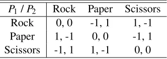
Transitive/Intransitive To better explain with examples, we restrict the definition to symmetric games. A pure strategy s is preferred over another one s0 (denoted s>s0) if the pay-off E(s,s0)>0,E is the evaluation function. A game is transitive if for all pure strategiess,s0 ands00 , we haves>s0 ands0>s00implies s>s00. Otherwise, the game is intransitive. A well-known intransitive game is the Rock-Paper-Scissors game (RPS game), which is also the smallest intransitive game.

P1/P2 Rock Paper Scissors

Rock 0, 0 -1, 1 1, -1 Paper 1, -1 0, 0 -1, 1 Scissors -1, 1 1, -1 0, 0

Table 2.2: The payoff matrix of the Rock-Paper-Scissors game.

Zero-sum/Non-zero-sum/Constant-sum A constant-sum game is a game where the sum of the pay-off of agents is a constantc. That is,M1[i][j] +M2[i][j] =cfor alliand j. A zero-sum

game is where this constantc=0. Clearly, the Prisoner’s Dilemma game is a non-zero-sum game while the Rock-Paper-Scissors game is a zero-sum game. For simplicity, we normally denote such a game as one matrix representing the payoff of the row playerP1. For the

Rock-Paper-Scissors game, we haveMr ps. In this thesis, we deal with mostly non-zero-sum games.

Mr ps=  

0 −1 1 1 0 −1 −1 1 0

 

2.1.2 Strategies and Equilibria

2.2 Computing Nash Equilibria 11

is a set of actions associated with their corresponding probability. A pure strategy is a special case of a mixed strategy where there is only one action with probability 1. In this thesis, both strategies in this thesis are uniformly denoted assfor simplicity.

A two-player game has a pure or mixed strategyNash equilibriumin case both players have no better payoff by changing their strategies. Formally, for two playersP1andP2and their strategies

s1ands2,(s1,s2)is in a Nash Equilibrium if for any strategiess01ands20,E(s1,s2)≥E(s1,s02)and

E(s2,s1)≥E(s02,s1). Not all games have a pure strategy Nash Equilibrium. However, all games

have at least one mixed strategy Nash Equilibrium. For example, the Rock-Paper-Scissors game does not have any pure Nash equilibrium but has a mixed strategy Nash equilibrium where the three strategies are played uniformly.

For two players with mixed strategiesS₁andS₂respectively in a zero-sum game, we have the Min-Max Theorem to help us find the Nash Equilibrium (i.e., solve the game) [3]. The theorem states that the pair of strategy(s0₁,s0₂)is a Nash Equilibrium wheres0₁=argmaxs1∈S1mins2∈S2E(s1,s2)and

s0₂=argmaxs2∈S2mins1∈S1E(s2,s1). Formally:

Theorem 2.1.1— The Min-Max Theorem.

max s1∈S1

min s2∈S2

E(s1,s2) =−1∗max

s2∈S2

min s1∈S1

E(s2,s1) =min

s1∈S1

max s2∈S2

E(s1,s2)

In matrix form, letx∈Xandy∈Y be the (probability distribution of) mixed strategies andMbe the payoff matrix. The matrix form is as follows with v as the optimal payoff:

Theorem 2.1.2— The Min-Max Theorem (matrix form).

max x∈X miny∈Yx

T

My=min y∈Ymaxx∈X x

T My=v

From the description above, a mixed strategy of Nash Equilibrium shows the best a player can do to obtain optimal payoff. Intuitively, if a pure strategy beats such a mixed strategy, it is better than the “joint force” of the actions involved.

2.2 Computing Nash Equilibria

2.2.1 Introduction to Linear Programming

Alinear programming(LP) problem maximizes (or minimizes) a value with respect to some linear constraints. For example, we are to maximizev=5∗x1+3∗x2regarding two constraints:x1+x2=1

andx₁−x₂≤3. We can first substitute allx₁by 1−x₂and getv=5−2∗x₂andx₂≥ −1. That is, the maximum ofvis 7 whenx2=−1 andx1=2. Real cases can be much more complicated with

In this project, we take advantage of existing tools. ThePuLPlibrary [23] is an open source Python package that allows mathematical programs to be described in the Python programming language. It is easy to interact with and fast in finding solutions [23].

2.2.2 Game Solving with LP

Next we take advantage of the Min-Max Theorem and convert the searching of a Nash Equilibrium into a linear programming problem. In this section, we introduce this approach step by step by solving the Rock-Paper-Scissors. The payoff matrixMr pscorresponds to the row player as follows. We introduce a vector of probability corresponding to the three actions of the column player: Rock, Paper and Scissors:x= (x₁,x2,x3)∈X (similarly, for the row player, we havey= (y1,y2,y3)∈Y).

Mr ps=  

0 −1 1 1 0 −1 −1 1 0

 

The payoff for the row player is therefore:

v=max x∈X miny∈YxM

T r psy

. That is, the row player maximizes the value

v=min y M

T r psy

• When the row player chooses Rock:v= (0∗y₁) + (−1∗y₂) + (1∗y₃) • When the row player chooses Paper:v= (1∗y1) + (0∗y2) + (−1∗y3)

• When the row player chooses Scissors:v= (−1∗y1) + (1∗y2) + (0∗y3)

Now that the column player maximizes its payoff−v(minimizev), the player would take the smallest of all three:

v≤ −y2+y3

v≤y1−y3

v≤ −y₁+y₂

We also know thaty1+y2+y3=1 and each of them is non-negative (y1≥0,y2≥0 andy3≥0).

2.2 Computing Nash Equilibria 13

Now that we have some experience working using PuLP to solve games, we can generalize this approach to zero-sum games of any size. The following is a description of the procedure to find the equilibrium taking advantage of LP solvers.

Data: A pay-off MatrixM Result: Two mixed strategies

initialise a list of variablesx= [x1,x2, . . . ,xn]; initialise a LP solverL;

Set the objective ofLto maximisev; foreach column cdo

add constraintv≤x₁∗M[1][c] +x₂∗M[2][c] +. . .+xn∗M[n][c]toL end

add constraint∑ni=1xi=1 toL;

add constraintxi≥0 for eachxi∈xtoL; decodexfrom the result ofL;

In similar approach, get that of the row player.

Algorithm 1:A general procedure of zero-sum game solving with LP.

2.2.3 Asymmetric Games

While symmetric games involve two players with access to the same set of actions, biological interactions, even between members of the same species, are almost always asymmetric due to access to resources, differences in size, or past interactions [21]. Soon after the introduction of game theory to biology, the study of asymmetric games has drawn attention of many [11]. Conflicts with built-in asymmetries like those between male and female, parent and offspring, prey and predator and the corresponding dynamics have been studied [28, 11, 21]. There are also a wide range of such games outside of biology: chess, poker, backgammon, etc. While asymmetric games are hard at first glance, it is possible to construct a new compound game consisting of two copies of the original asymmetric games for some asymmetric games [25]. A strategy in this game is a pair consisting of the strategies of both players in the original game:t= (s1,s2). The payoff oft0= (s01,s02)is defined

asE(t,t0) =E(s1,s0₁) +E(s2,s0₂). In other words, the set of strategies is the set of Cartesian product

of the set ofP₁andP₂. However, the flexibility with which the new mixed strategy is constructed is constrained: it is not possible to put weight on a particular first player strategys1without putting the

same weight on the corresponding second player strategys2[25].

An example asymmetric game is the battle of the sexes (BoS) where a couple agreed to meet in the evening for some activities. The man prefers to watch a football match, while the woman would rather enjoy an opera. Both enjoy the company of the other. The payoff matrices are defined as follows:

Mman=

Mwoman=

2 0 0 3

Observe that the game has two pure strategy Nash equilibria, one where both go to the opera and another where both go to the football game. There is a third (mixed strategy) Nash equilibria where the man goes to the football with probability 60% while the woman goes to the opera with probability 60%.

2.2.4 Bimatrix Games

A more general type of game is thebimatrix gamewith one payoff matrix for each player. Among the the most famous algorithms, the Lemke-Howson Algorithm [26] can efficiently compute Nash equilibria for some problems. While the algorithm is efficient in practice, the number of pivot operations may need to be exponential in the number of pure strategies in the game in the worst case. It has been proved that it isPSPACE-completeto find any of the solutions [12]. Some more recent attempts shows that obtaining approximate Nash equilibria can be done in polynomial time [7, 26].

2.3 Neural Network

2.3.1 Introduction to Neural Network

2.3 Neural Network 15

Figure 2.1: The structure of Elman neural network [19].

Deep learningis a recent trend in machine learning that builds neural networks of many levels. As a consequence, typically such networks have thousands to millions of parameters [24]. Despite that large neural networks can be hard to train, the past decades witnessed neural networks widely applied to tasks in robotics and swarm agents such as decision making, computer vision, classification, path planning and intelligent control of an autonomous robot, etc [18, 22, 20, 16].

2.3.2 Elman Neural Network

Figure 2.1 shows the structure of a recurrent Elman neural network [6]. This neural network consists ofiinput neurons,hhidden neurons, and two output neurons (O1andO2).O1is fed back into the

input and controls the stimulus.O2is used for making a judgement. In addition, a biased neuron with

a constant input of 1.0 is connected to each neuron of the hidden and output layers. Such network has(i+1)h+h2+ (h+1)parameters. The activation function used in the hidden and the output neurons is the logisticsigmoid function:

sigmoid(x) =1/(1+e−x),∀x∈_R

control of a neural network to form a collision-free path [16]. This task may involve two (or more) neural networks. The first neural network is used to determine the “free” space using ultrasound range finder data while the second avoids the nearest obstacles and searches for a safe direction for the next robot section [16]. Neural networks are also widely used for system identification and pattern recognition [20, 19, 22]. A classifier observes the motion of an robot for a fixed time interval and outputs a boolean judgment if it has certain properties in behavior [20].

2.4 Introduction to Evolutionary Computing

2.4.1 Evolution

Darwin’s theory of evolution offers an explanation of the origins of biological diversity and its underlying mechanisms. Natural selection favours those individuals that better adapt to the environ-ment for reproduction and therefore accumulate beneficial genes [5]. Genes are the functional units of inheritance encoding phenotypic characteristics while genome stands for the complete genetic information of an individual [5]. The genome of an offspring maybe impacted by crossing-over, mutation, etc.

2.4.2 Evolutionary Computing

As the name suggests, Evolutionary Computing (EC) draws inspiration from the process of natural evolution. The idea of using Darwinian principles to automated problem solving dates back to the 1940s. The idea was first proposed by Turing in 1948 as genetical or evolutionary search. The subject embraced huge development since 1990s and many different variants of evolutionary algorithms were proposed [5]. The ideas underlying are similar: given a population of individuals within an environment with limited resources, competition for those resources causes natural selection (survival of the fittest).

Data: An initialisedλ+µ population with random candidate solutions Result: A pair of solutions

Evaluate each candidate;

whileTermination Condition is not satisfieddo selectλ parents ;

recombine pairs of parents and obtainµ offspring with mutation; evaluate new candidates;

put togetherλ parents andµ offspring for the next generation; end

returnthe best fit individual

2.4 Introduction to Evolutionary Computing 17

Evolutionary Computation (EC) offers a powerful abstraction of Darwinian evolutionary models with application from conceptual models to technical problems [33]. The best-known class of EAs are arguablygenetic algorithms(GAs) [33]. Most GAs represent individuals using a binary encoding of some kind and perform crossover and mutation during reproduction. Another type of EAs are evolutionary strategies. This approach is often employed for problems with a representation of real numbers. Evolutionary strategies first initialize a set of candidate genomes (i.e. solutions) at random and then simulate the competition with an abstract fitness measure. On the basis of such fitness values, some optimal candidates are chosen asparentsto reproduce the next generation. This is done by applying recombination and/or mutation to them.Recombinationis an operator that combines features of two or more selected candidates (i.e. parents). During reproduction,mutation(as an operator to each gene) may happen, which results in a partially different candidate. This process creates a set of new candidates, namely, theoffspring. The algorithm terminates when some given terminating condition is reached. An example is theλ+µ algorithm (Algorithm 2) where theλ parents are selected to reproduce µ offspring. Notice that although those with better fitness are more likely to be selected, this probabilistic algorithm may not choose to let it reproduce, which is consistent with nature but may not be good for an optimization problem.

Common bisexual reproduction processes consist of two operations: recombination and mu-tation. A geneg= [g1,g2, . . . ,gn]∈Gis associated with a sequence of mutation strengths (fac-tors)σ = [σ1,σ2, . . . ,σn]∈Σ. When producing with another gene g0 = [g0₁,g0₂, . . . ,g0n]∈Gwith σ0= [σ₁0,σ₂0, . . . ,σ_n0]∈Σto formg00and σ00, the recombination process is a choice between the parents’ genes of even chance:

g00_i :=giORg0i,i=1, . . . ,n; (2.1)

σi00:=σiORσi0,i=1, . . . ,n (2.2)

Theng0is mutated. For each generation, we first obtain a numberrgenerated from the standard normal distribution (with mean of 0 and standard deviation as 1; see Appendix A.2 for implementation details). For each gene, in similar approach, we generate a numberri.

σi00:=σi00∗exp(τ0∗r+τ∗ri),i=1, . . . ,n; (2.3) g_i00:=g00_i +σi00∗ri,i=1, . . . ,n (2.4)

In the formula above,τ0=1/2 √

2∗Nandτ=1/2 p

2√Nwith N being the size of the population. See Appendix A.2 for a detailed example.

3. Coevolution and Turing Learning

3.1 Introduction to Coevolutionary Computation

3.1.1 Coevolution and Coevolutionary Computation

Evolutionary algorithms (EAs) are heuristic methods for solving computationally difficult problems inspired by Darwinian evolution. This approach is typical for a variety of problems from optimization to scheduling. However, in many problems in nature, the fitness of an individual does not only depends on the environment, but also on the behavior of the others in the environment. The existence of other individuals may change or have an influence on the attention, cognition, reproduction and other social activities [27]. For example, some flowering plants and honeybees have a symbiotic relationship: flowering plants depend on an outside source to spread their genes through pollination while bees receive nectar, which they convert into honey to feed their queen bee.

of many genes. Abstractplayersmanage strategies. In this thesis, we only deal with two-player coevolutionary processes. Coevolutionary processes have more complexity [33]. To better illustrate the concept of coevolution, we provide a simple abstract sequential cooperative coevolutionary algorithm below [33].

Data: Initialize a population with random candidate strategies for eachP₁andP₂ Result: Best strategies from both population

Evaluate each candidate;

whileTermination Condition is not satisfieddo select parents and reproduce the offspring ; select collaborators from the population; evaluate offspring with collaborators; select survivors from the new population; end

returnthe best fit strategies in each population

Algorithm 3:A simple abstract cooperative coevolutionary algorithm.

3.1.2 Coevolutionary Architectures

Coevolutionary Computation(CoEC or CEC) is the study ofCoevolutionary Algorithms(CoEAs or CEAs) where the fitness of a strategy depends on the strategy of the other player and thus differs from traditional evolutionary methods [33, 28]. Anobjective measureevaluates an individual regardless the effect of the others, aside from scaling or normalization effects. Otherwise, it is asubjective measure. A measurement isinternalif it influences the course of evolution in some way, otherwise, it isexternal. A CoEA employes a subjective internal measure for fitness assessment [33]. Depending on the relationship of the two players in an coevolutionary process, CoEAs can be further classified ascooperativeCoEAs and competitiveCoEAs. It is cooperative when the increase of fitness of one population of a player in the new generation leads to positive impact on the fitness of the other. Otherwise, it is a competitive CoEA. Most work in the field of CoEA studies competitive coevolution [33, 28]. In most nature-inspired computation, updating timing is sequential and the decomposition of problems are dynamic [28].

In simple coevolutionary process, a strategy usually correspond to a single object, while in some cases, it can be a group of similar/identical objects. For instance, when a strategy is a distribution of some property, the corresponding implementation may be a group of individuals following such distribution. The interactions may be one-to-one between two objects or that of a selection of some objects regarding a certain bias [33]. This thesis studies only one-to-one interactions. As a result, a payoff is assigned to each strategy. In many algorithms, the fitness is simply the sum of the payoff of a strategy against that of the opponent. Section 4.2 gives a different view on this and provides an implicit fitness evaluation. The selection of samples in evaluation is to be in Chapter 6.

3.1 Introduction to Coevolutionary Computation 21

its drawbacks. For instance, the dynamics is often harder to capture and the subjective fitness may not be accurate enough. One of the problems is the so-calledloss of gradientwhere the strategy of one player converges making the other player lose “guidance” while coevolving. Another problem is “cyclic behavoir” where one player re-discover the same set of strategies after a few seemingly “better and better” coevolutionary generations. To further study this property of CoEAs, I present (a modified version of) the Intransitive Number (ING) Game as described in [8] to examine the properties of intransitive relations. To better understand the properties of the impact of entities during coevolution, I designed two games to be presented in Section 3.3. Strategies in the population may be treated uniformly or grouped as different populations according to their fitness and/or other properties (see Chapter 4).

3.2 The Intransitive Numbers Game

One problem associated with coevolutionary algorithm is that some traits are lost only to be needed later. To rediscover/relearn these traits may require more effort. Ficici and Pollack [8] proposed a game-theoretic memory mechanism for coevolution with evaluation using Watson and Pollack’s Intransitive Numbers Game (ING) [32]. The ING game is in a co-evolutionary domain that allows intransitive relations. This section explains the game and the nature of how intransitive relations make coevolution harder. Evaluation results are presented after the introduction of a generalized version of such memory mechanism in Section 4.4.1.

Representation of Strategies Each pure strategy of the ING game is an n-dimensional vector of integersα =hi1, . . . ,ini. Each integer iis represented as a list ofb bits. For example, α=h4,3i=h0100,0011i1.

Evaluation Function For two pure strategiesα andβ, the payoff for the first playerE(α,β)is calculated in three steps as follows:

E(α,β) =

0 ifmin(hi) =∞ sign(∑ni=1gi) otherwise

(3.1)

gi=

αi−βi ifhi=min(h)

0 otherwise (3.2)

hi=

|αi−βi| if|αi−βi| ≥ε

∞ otherwise (3.3)

3.3 The PNG and RNG Game 23

isE(β−α) = 0 -E(α,β). We keep consistent with [8] and take our strategy space to be n-dimensional vectors of natural numbers, where each dimension spans the interval[o,2b−1]; This results in(2b)ndistinct pure strategies. The game has a single Nash strategy whenε<k and multiple otherwise [8]. The single Nash strategy is the pure strategy with valuekin alln dimensions, i.e.,h2b−1,2b−1, . . . ,2b−1i

| {z }

n

.

This 3-step calculation may not be obvious. The following is an example: takeα1=h4,2i,

α2 =h2,6i, α3 =h7,3i. To calculate E(α1,α2), we first obtain h1 =2 and h2 =4 and

min(h1,h2) =2. Sog1=2 andg2=0 which makes∑ni=1gi=2>0. ThusE(α1,α2) =1.

Likewise, we getE(α2,α3) =1 andE(α1,α3) =−1. This gives an example of intransitive

relations between three individuals in the search space.

We consider this game as a coevolutionary process where two playersP1andP2each maintain

a list of strategies2. The scorewof a strategyα ofP1is thew=∑in=1E(α,βi)withβi∈P2

and vice versa. The score of all strategies isW= [w₁, . . . ,wn]and the fitness of each strategy is fi=wi−min(w) +0.1. This guarantees the fitness of a strategy to be positive.

Population Management and Reproduction In each iteration, each player managexstrategies and the bestyare selected to generate thegoffspring asexually. Each bit has a mutation rate of 0.1 for example (i.e., each bit has 10% of chance to become 1−b).

Termination The game terminates after 1000 generations for instance. Evaluation results are in Section 4.4.1.

3.3 The PNG and RNG Game

Percent Number Game (PNG) and Real Number Game (RNG) are two similar games introduced for the understanding of how the relation between two players impact coevolution. They also serve as test cases for non-zero games and bisexual reproduction.

Representation of Strategies Similar as the ING game, for the PNG/RNG game, there are two playersP1andP2, each maintain a set of strategies. Each strategy is a point in an-dimensional

space within the range[0,B], whereBis the bound. For the PNG game, the bound isB=1 while RNG takesB=100. In 2D space, a strategy could beα= (0.5,0.3)for example. Before the a game starts, we fix two pointsx= (x1,x2)andy= (y1,y2)in then-dimensional space as

pre-defined attractors and assign one to each player. For each gene, we also associate each gene with a (positive) mutation rate, denoted asσas described in Section 2.4.2. Interestingly, whenε>1, the two population would eventually cluster to the same point rather than their attractors (see Figure 3.2).

Evaluation Function For a game inN-dimensional space, we define an evaluation functionE(α1,α2) =

(w1,w2)withα1= (s1,s2)andα2= (t1,t2)as the strategies of the two players. WhenN=2,

w₁andw₂are defined as follow:

w1= ((1− |s1−x1|)2+ (1− |s2−y1|)2) +ε∗((1− |s2−x2|)2+ (1− |s2−y2|)2).

w2= ((1− |t1−x1|)2+ (1− |t2−y1|)2) +ε∗((1− |t2−x2|)2+ (1− |t2−y2|)2).

(a) the population over 30 iterations withε=2

(b) the population over 30 iterations withε=0.2

3.4 Turing Learning 25

ε is the coefficient for correlation. The payoff values represent how close a point is from its attractor and the opponent’s strategy. The largerε is, the more attractive an opponent strategy than the pre-defined attractor (as a point in 2D space).

Population Management and Reproduction In each iteration, there are 20 strategies for each player and the best fit ones are selected to generate the offspring bisexually. For example, a pair of selected parents areα1= (s1, . . . ,sn) andα2 = (t1, . . . ,tn), with mutation rate of σs1, . . . ,σsnandσt1, . . . ,σtnrespectively. We reproduce a childα= (k1, . . . ,kn), with mutation rateσk1, . . . ,σkn.

1. First, we need to compute some intermediate values. Eachk_i0has a equal chance to be eithersiortiwhileσ_ki0 = (σsi+σti)/2.

2. Then we need random numbersµ for this reproduction process andµifor each gene, both following Gaussian distribution with a mean of 0 and standard deviation of 1. 3. Finally,σki=σ_ki0 ∗exp(τ0∗µ+τ∗µi)whereτ0=1/(2∗

√

2n)andτ=1/(2∗p2∗ √

n). Termination The game terminates after a given number of iteration.

3.4 Turing Learning

3.4.1 Inspiration and Background

Robots and other automation systems have greatly transformed our world over the past decades. Swarm Intelligence(SI) studies the design of intelligent mulit-robot/agent systems inspired by collective behavior of social insects [4]. Collectively, they can achieve much more complex tasks in cooperation than that of an individual.Ethologyis about the study of animal behavior. Ethologists observe that some animals have similar appearance or behavior as another different species to increase the survival chance while there are still significant distinction between the two species. This is known as theconvergent evolutionwhere the independent evolution of unrelated or distantly related organisms evolve similar features including body forms, coloration, organs, and adaptations. For instance, in Central America, some species of harmless snakes mimic poisonous coral snakes that only an expert can tell apart [14]. Natural selection can result in evolutionary convergence under various circumstances. Some mimicry is disadvantageous to the model species since it takes longer for the predator to learn to avoid them. Ethologists often need to observe the animals and analyze the data manually to extract meaningful information from the records of animals under investigation, which can be time-consuming and tedious. With the help of different automation systems, it is much easier to conduct experiments more efficiently and accurately. The question is whether it is possible to construct a machine/system that can accomplish the whole process of scientific investigation, reasoning, automatic analysis of experimental data, generation of a new hypothesis, and the design new experiments. The development of “robot scientists” Adam and Eve by the team of Prof. Ross King gave a positive answer [17].

pass the Turing test if it could learn and adapt as we humans do. In June 2014, a Russian chatter bot named Eugene Goostman, which adopts the persona of a 13-year-old Ukrainian boy, fooled a third of the judges in 5-minute conversations [34]. The competition’s organizers believed that the Turing test, for the first time, had been passed. However, the discussion and study of computational models continues for better simulation of the capabilities of human being in cognition, decision making, cooperation and many more aspects. Most recently, Turing Learning provides a new automated solution to the learning of animal and agent behavior [20].

Table 3.1: Turing Learning v.s. Coevolutionary Computing v.s. Turing Test v.s. Convergent Evolution.

Turing Learning Coevolutionary Computing

Turing Test Convergent Evolution Entities Real agents,

strategies and the correspond-ing GAOs

Genes Human and

computer programs

Model species, mimic species and the preda-tor

Aim Learn the be-haviour of indi-viduals thought interaction

Study the dynam-ics of two popu-lation of individu-als

Distinguish computer pro-grams from human by ana-lyzing dialogues

Behave or ap-pear like the model species

Evaluation The classifica-tion result of an experiment

fitness computa-tion

The accuracy of distinction

The predator’s distinction

3.4.2 Turing Learning Basics

3.4 Turing Learning 27

strategies execute on areGenerative Adversarial Objects(GAOs)3. From a biological point of view, while the strategies are like the genotype, GAOs are the corresponding phenotype. Overall, a system in such a setting is aTuring Learner.

Table 3.1 illustrates a comparison with other concepts. In Turing Learning, the coevolving entities are the unique strategies (and the GAOs generated accordingly) while the real agents under investigation remain the same in each generation. In contrast, in classical coevolution, the two species under investigation generate offspring in each generation. Turing learning shares similarities with convergent evolution: the classifiers in Turing Learning function in a way similar to predators in convergent evolution.

Figure 3.3: The architecture of a Turing Learner.

3.4.3 Architecture and System

A Turing Learner maintains three entities: a model player, a classifier player and the agents under investigation. A Turing Learner first initializes a model player and a classifier player; each manage a population of random strategies. In each iteration, for each strategy, the model player generates one or many replica agent(s) accordingly. An experiment is an interactive process of these agents in a sequence of timesteps. The model player then generates a classifier from a chosen strategy and take the observed data in the experiment as input. The output is the classification results for of the individuals in the experiment. The fitness of a model strategy is the probability of wrong judges by the classifiers. The fitness of a classifier is the sensitivity plus the specificity. Formally, for an experiment usingCclassifiers withAreal agents andRreplicas, the fitness values of a model and a classifier, fmand fc, are defined as:

fm=1/C C

∑

(1−Or)

fc=1/2((1/A A

∑

(1−Oa)) + (1/R R

∑

Or))

In the formula above,Oris the output of the classifier when evaluating on replica agents.Oais the output of the classifier when the input is from a real agent. At each generation, both players then select among a given number of strategies as parents according to their fitness value and generate the offspring. The learning process terminates after a given number of generations.

Different from existing behavior learning approaches, Turing Learning focus on the learning of agent behavior through interaction. This learning approach has its requirement in setting: an experiment consists of several real agents and replica agents. Agents must interact with each other to form observable evidence. Classifiers are not only to examine the evidence of the replica agents, but also the real agents. The goal is to learn the interactive behavior of some real agents rather than obtaining an optimal solution of a problem. Note that the result of Turing Learning might not be optimal or efficient. This thesis is to introduce Nash Memory to Turing Learning and examine efficiency improvement if any. For the purpose of comparison, we take the aggregation game as the test case.

3.5 Aggregation Game

In this thesis, we study the aggregation game in detail [20]. The game is a typical problem in swarm robot system where the mission of robots is to aggregate into a cluster in an environment free of obstacles [10]. In this aggregation experiment, we use the simulation platform Enki4(see Section A.1 for details). Enki has a built-in 2-D model of the e-puck robot. An agent in simulation is represented as a epuck robot of a disk of diameter 7.0 cm with mass 150 g. The speed of each wheel can be set independently (see Section A.1.1 for the complete specification). More specifically, the agents follows a reactive control architecture. The motion of each agent solely depends on the state of its line-of-sight sensor. Each possible sensor state is mapped to a predefined specification of the control of motors. In this thesis, we deal with only the sensor at the front. When the agent is free from obstacles along sight, the sensor reads 0 (I=0) and the velocity of the left wheel isvl and that of the right isvr. When the sensor reads 1 (I=1), the velocity values arev0l andv0rrespectively. This reactive behavior of an agent depends solely on these parameters. For simplicity of representation, we collect all the parameters as a vector p={vl,vr,v0l,v

0

r} withv∈[−1,1],v∈p. The marginal values correspond to the maximal values of the wheel rolling backward and forward respectively. In this thesis, we follow the setting of [20] and assume that the replica has the same differential drive

3.5 Aggregation Game 29

and the line-of-sight sensor. The system identification task is therefore to infer the control parameters inp. This setting makes it possible to objectively measure the quality of the obtained models in the post-evaluation analysis. For a replica followingq={ul,ur,u0l,u

0

r}, the error is measured as follows:

For each parameter piandqi(i∈ {1, . . . ,N},N=|p|=|q|), the Absolute Error (AE) is: AEi=|pi−qi|

The Mean Absolute Error (MAE) over all parameters is:

MAE=1/N∗ N

∑

AEi

All simulations are conducted in an unbounded area where there areAreal agents andRreplica agents. The initial position of a robot is uniformly distributed within an area of((A+R)∗Z)cm2 whereZ=10,000 (average area per individual). In this thesis, we follow the setting proposed by [10] and take p={−0.7,−1.01.0,−1.0}to achieve this aggregation behavior5.

4. Nash Memories

4.1 Nash Memory

4.1.1 Memory Methods and Solution Concepts

In coevolution, each player manages a population of candidate solutions. Using the “methods of fitness assignment” some better fit ones are “remembered” and remain in the population while the rest are “forgotten” before the next generation. The problem of designing a heuristic “memory mechanism” is to prevent forgetting good candidate solutions with certain traits. The contribution of a trait to the fitness may be highly contingent upon the context of evaluation. Even when candidate solutions with/without certain traits are equally fit, the candidates are at risk of drifting due to sampling error in the population dynamic leading to the lose of traits [8]. A solution concept specifies precisely a subset of candidate solutions qualify as optimal solutions to be kept in the population [25]. This is a more general definition of “methods of fitness assignment” introduced in Section 3.1.2. The study of solution concepts is important for evolutionary mechanisms that deal with candidate solutions with many traits while only maintain a limit amount of solutions in the memory [9]. As we described in Section 3.2, the ING game is a coevolutionary domain that is permeated by intransitive cycles. For a coevolutionary domain where a strategy consists ofnintegers, there arentraits to be “watched” by the solution concept.

contrast to this approach, Stanley and Miikkulainen proposeddominance tournament(DT) [29]. The principle is to add the most fit individual of the generation only if it beats all the individuals in the memory. This prevents the case of intransitive relations as those of the ING game for example.

4.1.2 Introduction to Nash Memory

Nash Memory [8] is a solution concept introduced by Ficici and Pollack as a memory mechanism for coevolution. It was designed to better deal with cases where one or more previously acquired traits are only to be needed later in a coevolutionary process. This memory mechanism maintains two set of solutions and uses a game-theoretical method for the selection of candidates to better balance between different traits in coevolution. Before introducing the memory mechanism in detail, some concepts need to be clarified:

SupportSup(s) The support of a mixed strategysis the set of pure strategiessiwith non-zero probability: Sup(s) ={si|Pr(si|s)>0}. For a set of mixed strategies, we defineSup(S) = S

iSup(si),si∈S1.

Security setSec(s) The security set of strategy ofs is a set of pure strategies against which s has an expected non-negative payoff. In other words,Sec(s) ={si|E(s,si)≥0}. Similarly, Sec(S) =T

iSec(si),si∈S2.

Domination A strategysadominates a strategysbif for any strategy s,E(sa,s)≥E(sb,s) and there exists a strategys0such thatE(sa,s0)>E(sb,s0).

Support-secure If the security set contains the support set, then the strategy issupport-secure.

Most population management in coevolutionary computation maintain a population of candidate solutions according to some explicit organizing principle discovered over generations. In contrast, Nash Memory uses an implicit measurement [8] using pairs of mixed strategies retrieved from Nash equilibria. These pairs are recommendations to the players on which action to take. The following (non-zero-sum) example gives a taste of this approach. The game is an extended version of the battle-of-sex game described in Section 2.2.3. Now there are four options for the man: a) watch a football match, b) watch an opera, c) prepare for an exam and d) write a thesis.

Mman=     3 0 0 2 1 2 8 −1

   

4.1 Nash Memory 33

Mwoman=     2 0 0 3

−1 −6 −8 4

   

Classical explicit methods would calculate the fitness of each strategy by summing the payoff uniformly. That is, the fitness values of the four strategies are 3, 2, 3, 7 respectively. However, Nash Memory gives a different solution concept. It computes the Nash equilibria first:

1. The man plays b) and c) with a probability of 0.625 and 0.375 respectively while the woman plays b).

2. The man plays c) and d) with a probability of 0.705 and 0.294 respectively while the woman goes to the opera with a chance of 0.7.

3. Both go to the opera (i.e. the man plays strategy b).

Imagine the man has to remove an option for next week (i.e. forget a strategy in the memory). According to the fitness using explicit method, he should forget about going to the opera next week. However, a) is not participating in any Nash equilibria, thus using the approach of Nash memory, the man will not consider watching a football match next week instead.

4.1.3 The Operation of Nash Memory

The Nash memory mechanism consists of two mutually exclusive sets of pure strategies:N andM [8].N is defined as the support of the Nash strategysNthat is at least secure against the elements ofN and M (Sec(∫_N)⊇N ∪M). The objective of this set is to represent a mixed strategy that is secure against the candidate solutions discovered thus far. The security set is expected to increase monotonically as the search progresses, thereby forming a better and better approximation of strategies for the game. On the other hand,M plays the role of a memory or an accumulator. It contains pure strategies that are not currently inN , but were in the past. They may be inN again in the future. By the definition as in [8],N is unbounded in size andM is defined as a finite set. The size limit ofM isc, which is known as the capacity of the memory. For simplicity, in this section we assume there is only one Nash equilibrium.

Initialization

BothN andM are initialized as an empty set. Let the first setT to be delivered by the searching heuristics3. We initializeN so thatSup(N)⊆T andT ⊆Sec(N).

Data: The size limit ofM,bm

Result: The best strategy of at the end of iteration

InitializeN andM as described in Section 4.2. whiletermination condition is not satisfied do

Obtain a set of new strategiesT;

Evaluate strategies inT against the current Nash equilibria and store the winnerW; ObtainU=N ∪M∪W;

Evaluate the candidate strategies inU and obtain the payoff values; Compute the Nash equilibria and updateN;

UpdateM as described in Section 4.1.3 usingbm. end

returnthe best fit pure strategies inN .

Algorithm 4:Nash Memory.

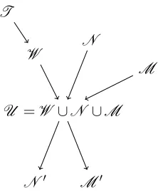
U =W ∪N ∪M T

W N

M

N 0 _M0

Figure 4.1: The Updating ofN andM in Nash Memory.

Updating_N and_M

We compute a setW ={t∈T|E(t,sN)>0}as the winners against the current best strategysN. Using Linear Programming, we can obtain a new Nash strategys0_Nout of the setU =W ∪N ∪M4_.

Next,N0:=C(s0_N)andM0:=U −N0. This process guarantees thatW ⊆Sec(N ). Figure 4.1 gives an illustration of this process. Note that the updatedM0may have a capacity larger thanbm. A number of policies can be used to reduce the size ofM0:

• remove those with the least fitness value calculated in the classical way. • remove those that participated the least over the past generations. • remove items at random from M then those released fromN .

4.2 Parallel Nash Memory 35

Termination

The algorithm terminates after a fixed number of iterations. Other terminating conditions may be adopted. The best fit pure strategies are returned.

4.1.4 Nash Memory in Application

Intuitively, theN behave like a defending army and defend the attack from the newly discovered strategiesT. Those who survive form the setW. However, obtaining a survivor can be hard in some cases. It is possible that multiple genes have to evolve to a certain extend at the same time to obtain a pure strategy, and thus requires the evolution of multiple generations. A way to deal with this is to evolve a few generations againstN and then updateN using such a winner (if any). The Nash Memory mechanism has been examined using the ING game to outperform the Best-of-Generation and Dominance Tournament [8] where the coevolutionary process was transformed to an evolutionary domain. There they introduced this concept ofepochsto capture the searching heuristic described above. One epoch is 30 generations. At each epoch, only 10 best fit strategies are selected to generate 90 new strategies as offspring.

Nash Memory guarantees monotonicity approaching to convergence [8]. It is a memory mecha-nism designed to avoid being trapped in an intransitive loop. However, it was set to form a zero-sum and symmetric game each time updatingN andM. As we have discussed in Section 2.2.3 and Section 2.2.4, many games are either asymmetric or not necessarily zero-sum. In the following sections, we explore possible ways to apply Nash Memory to such cases.

4.2 Parallel Nash Memory

Nash Memory guarantees monotonicity with respect to a given solution concept, but is limited to the use of Nash equilibria of symmetric games. Many problems of practical interest are asymmetric (see Section 2.2.3 for concepts and detailed discussions). Oliehoek, et al. extended Nash Memory and introducedParallel Nash Memory[25]. Any coevolutionary algorithm can be combined with it and guarantee monotonic convergence5. We introduceN1,M1, andT1for playerP1andN2,M2,

andT2for playerP2. The algorithm works similar as that of the Ficic’s Nash Memory as introduce

above:

Initialization

N1,M1,N2 andM2 are initialized as empty sets. Let the first setsT1 andT2 to be delivered

by the searching heuristics. We choose N1 andN2 so that Sup(N1)⊆T1, T1⊆Sec(N1), and

Sup(N2)⊆T2,T2⊆Sec(N2).

UpdatingN andM

In zero-sum games, both players are able to provide a security level payoff and the sum should be zero. Assume that the search heuristic delivers a single test strategy for both players. We can test the compound strategyt= (t1,t2)against the compound Nash strategys= (s1,s2)as:

E(t,s) =E(t1,s2) +E(t2,s1)

In the original paper, whenE(t,s)>0, the Nash strategysis not secure againstt and therefore should be updated [25]. However, the following example shows that it is not the case.

Again, we modify the Battle of Sex game. This time, both of them find it an option to go swimming. The payoff matrices are now:

Mman=  

3 0 2 0 2 −3 2 1 0

 

Mwoman=  

−3 0 −2 0 2 3 −2 2 0

 

Before discovering the third option, the Nash equilibrium is that the man watches football match and the woman listens to the opera; both with payoff zero. Evaluating the new option against the current Nash, we haveE(t1,s2) =1 andE(t2,s1) =−2 and that makesE(t,s) =−1<0. However, there

is a need to update the Nash equilibria since the new equilibrium is now(1/3,0,2/3)for the man with a payoff of 2/3 and(0,2/3,1/3)for the woman. This might be a minor error in the paper6. We update the Nash when eitherE(t1,s2)>0 orE(t2,s1)>0.

Similarly, for non-zero-sum games, the situation is as follows. When a strategy is evaluated against the current Nash equilibria, as long as it gets the same or better payoff, it should be in the support of Nash in the next generation. For example, the man can now discover a new strategy to play, with which, the player can tie the payoff of a Nash. Thus, the strategy has to participate in the Nash forming a fourth Nash equilibrium. However, since it contributes to only one Nash equilibrium,

6_{In the paper,T was calculated using best-response heuristic so we always have bothE(t}

4.3 Universal Nash Memory 37

in case the man has to remove a strategy, it is logical to remove this newly discovered one. Note that the corresponding payoff of the opponent may decrease.

Mman=   3 0 0 2 1.5 1  

Mwoman=  

−3 0 −2 0 2 3 −2 2 0

 

Termination Condition

The algorithm terminates after a given number of generation, after reaching convergence, or satisfies some given conditions.

Data: The size ofM1andM2:bm1andbm2

Result: The best pure strategies at the end of iteration

initializeNiandMi(i∈ {1,2}, same below) as described above. whiletermination condition is not satisfieddo

obtain two sets of new strategiesT1andT2;

evaluate strategies inTiagainst the current Nash equilibria ofP3−i and store the winner Wi;

getUi=Ni∪Mi∪Wi;

evaluate the candidate strategies inUiagainstU3−iand obtain the payoff values; compute the Nash equilibria and updateNi;

updateMias described in Section 4.1.3 and reduce size usingbm1andbm2;

end

returnbest fit pure strategies inN1andN2.

Algorithm 5:Parallel Nash Memory.

Monotonic convergence is guaranteed for Parallel Nash Memory. In other words, we have U1⊆Sec(N1)andU2⊆Sec(N2)at each iteration. The algorithm has been evaluated using the

8-card poker game with best response search heuristic [25].

4.3 Universal Nash Memory

4.3.1 Introduction to Universal Nash Memory

do so, we first define a memory mechanism for bimatrix games: Universal Nash Memory(UNM in short). In this section, we present the algorithmic design of UNM and evaluation using the ING game. Further extension and integration with Turing Learning will be presented in Chapter 5. To guarantee monotonic convergence, we need to make sure thatNi∪Mi⊆Sec(Ni)(i∈ {1,2}).

a a a a a a a a a a Features Games

ING PNG, RNG Aggregation Game

Representation integer vectors vector of bounded real numbers

vector of bounded real numbers

Reproduction asexual bisexual bisexual Evaluation function simple direct calculation simple direct calculation

based on simula-tion and classifica-tion results

Termination both players converge/after some epochs

after some epochs

after some epochs

Symmetry symmetric symmetric assymmetric

Sum zero-sum

non-zero-sum

non-zero-sum

Table 4.1: A comparison of coevolutionary games.

Data: The size referencesr1andr2

Result: The best pure strategies at the end of iteration initializeNiandMi(i∈ {1,2}, same below) as PNM.; whiletermination condition is not satisfieddo

obtain two sets of new strategiesT1andT2;

evaluate strategies inTiagainst the current Nash equilibria ofP1−i and store (a selection of) the winnerWi;

getUi=Ni∪Mi∪Wi;

evaluate the candidate strategies inUiagainstU1−iand obtain the payoff matricesΞ1and Ξ2;

compute the Nash equilibria usingΞ1andΞ2;

obtain a newN_i0andM_i0 and reduce the size according to the size referecesri. end

returnbest fit pure strategies inN1andN2.

Algorithm 6:Universal Nash Memory.

4.3.2 Towards Universal Nash Memory in Application

4.4 Evaluation 39

was designed to better deal with cases where one or more previously acquired traits are only to be needed later in a coevolutionary process. This memory mechanism reports better balance between different traits in coevolution and guarantees monotonicity. This may help increase the learning efficiency of agent behavior. This project experiments the integration of Universal Nash Memory with Turing Learning and analyze the efficiency of learning of agent behaviors.

From Table 4.1, we see that Turing Learning differs from other games in many ways. The two players in Turing Learning are different in setting. The number of genes may differ significantly. Simulation results may lead to inaccuracy in fitness. It helps to take a closer look at UNM before applying to different coevolutionary games.

• A strategy of a classifier is typically a description of a neural network. Thus, the number of parameters could be huge. In comparison, the number of genes for a model could be significantly less.

• When searching strategies with a large number of parameters, it may take many evolutionary steps to tune all the parameters to beat the current Nash equilibria. In other words, it is more likely to have no winner for the player maintaining strategies with a large number of parameters.

• Different from zero-sum problems, bimatrix games are much more complex and harder to solve. For the sake of efficiency, we would have to consider reduce the size of payoff matrices. • The size of the game depends onUi, which is a sum of|Ni|,|Mi|and|Wi|(i∈ {1,2}). Careful

balance between the three sets can be tricky when the size referenceriis small. • There could be cases where there is no winner, or where there are too many winners. • Balancing between the evolution of players is also an important issue.

It is worth to consider small test cases before fixing an algorithm with limitation on the size of U for Turing Learning. This section presents an attempt integrating UNM with the ING games. The results and analysis are presented in Section 4.4.1. With this experience, UNM is carefully tested on non-zero sum cases: the PNG and RNG games. Finally we integrate UNM with Turing Learning. Implementation and evaluation details are in Chapter 5.

4.4 Evaluation

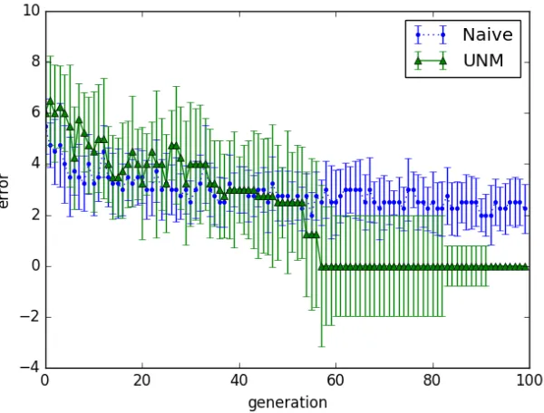
Figure 4.2: Convergence analysis of the ING game with/without UNM.

4.4.1 ING Game

The ING game is a very good test case where the algorithm deals with intransitive relations to reach convergence. Here we takeε =0 and 4 genes for each strategy, each of which consists of 4 bits. Every example completes 100 generations.

A crucial issue that was not discussed in [8] is the size ofN. In the ING game, whenN is free from size bound, the|N |can easily go beyond 50 (when there are four genes, each of which consists of four bits). Generally speaking, we would expect the size ofN not to be significantly bigger than that ofM andT. However, this is not the case due to complicated intransitive relations (even with an epoch of 30). In this project, we use one of the state-of-the-art bimatrix game solvers, thelrs solver (see Appendix A.4 for details) [1]. Although the time to compute each Nash equilibrium varies, the more the equilibria there are, the longer it takes in general. For instance, when the matrices are of size 10×10, it usually takes less than 0.1s to find all the Nash equilibria. When the matrices are of size 15×20, there could be over 1000 Nash equilibria and take several minutes. It may take up to half an hour to compute all the equilibria (over 10,000) when we have matrices of size 30×30.

At each generation, we obtain theN_i0andM_i0step by step regarding the size referenceri. In this test case, we takee1=1.5 ande2=2.

1. LetUi=Ni

4.4 Evaluation 41

3. AddMitoUiuntil|Wi|=e2∗ri

4. For two sets of strategiesU0andU1, compute the payoff matricesΞ1andΞ2

5. Compute (all) the Nash equilibria and extractNiand letMi=Ui\Ni 6. Reduce the sizeNitoriand add the discarded ones to the memoryMi 7. ReduceMito the memory size

5. Design, Implementation and Evaluation

Turing Learning is a novel system identification method for inferring the behavior of interactive agents. Over the past few years, some test cases have been developed and showed the success of Turing Learning in the learning of collective behavior. However, the source code of none of these projects is available for readers. Even worse, some of these projects are domain-specific and hard-coded. This chapter presents a plug-and-play Turing Learning platform, namely the TuringLearner.

5.1 TuringLearner: Design and Modelling

The project follows a modular design and an object-oriented modelling. At an abstract level, the TuringLearnerplatform is an instance of coevolutionary manager, which is an abstract class template.

APlayerclass is an instance of abstract class templates using meta-programming concepts. Given

Table 5.1: Integrated strategies and their players and games

IntVectorStg Pct-/RealVectorStg ElmanStg EpuckStg Reproduction asexual bisexual bisexual bisexual Players INGPlayer PNG-/RNGPlayer model player classifier player Game ING PNG & RNG aggregation game

strategies: the setN stores strategies participate in the Nash equilibria whileM serves as a memory of strategies not yet to be forgotten.

5.1.1 Strategies, Players and Games

Strategy

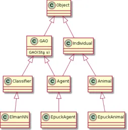
In this project, a strategy is explicitly a vector of genes. For the sake of simplicity in demonstra-tion and evaluademonstra-tion, several strategies comes along with theTuringLearner platform. We have

IntVectorStrategy, RealVectorStrategy andPctVectorStrategy for the ING, RNG and

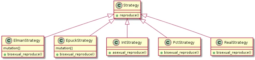
PNG games as described in Chapter 3. A strategy of typeIntVectorStrategyis a vector of lists of Boolean values evaluated to an integer number each. The other two consists of genes of real values. The reproduction can be asexual or bisexual. The reproducing process is managed by the corresponding player at the end of each generation. Two other types of strategies come together with the platform are theElmanStrategyandEpuckStrategy, which correspond to the Elman Neural Network and the spefication of an epuck robot respectively. It worth addressing that each of these genes is associated with a mutation value (Figure 5.1). Table 5.1 gives a summary of these strategies and their players and the corresponding games.

Figure 5.1: Class inheritance of built-in Strategy Classes.

Player

Players are managers of strategies and participate in a coevolutionary process.UNMPlayerdiffers

from SimplePlayerwhere there are two sets of strategiesN andM. A player ofUNMPlayer

5.1 TuringLearner: Design and Modelling 45

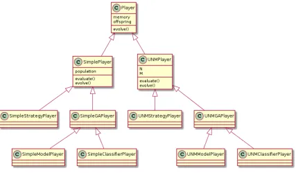
whileM serves as a memory of strategies not yet to be forgotten.UNMPlayeralso maintain a record of the Nash equilibria of the previous generation. ThePlayerclass are further divided into four sub-classes depending on their relation with the Generative Adversarial Objects:

1. SimpleStrategyPlayer: players that maintain a set of strategies for naive coevolution (e.g.,

the players of the (naive) ING game).

2. SimpleGAPlayer: players that maintain a set of strategies and the corresponding GAOs for

naive coevolution (e.g., the players of the (naive) aggregation game).

3. UNMStrategyPlayer: players that maintain two sets of strategies for coevolution using UNM

(e.g., the players of the ING game using Nash memory).

4. UNMGAPlayer: players that maintain two sets of strategies and their corresponding GAOs

(e.g., the players of the aggregation game using Nash memory).

Figure 5.2: Class inheritance of players.

Depending on the solution concept, a model player playingElmanStrategyand the maintain the Elman Neural Networks could be of classSimpleGAPlyerorUNMGAPlayer.

Coevolution Manager

game solvers. The default solver islrs. Since this project follows a modular design, other solvers may be integrated. Coevolution managers is also incharge of interacting with the simulation platform and takes GAOs instead of strategies to compute the payoff using the simulation results if specified.

Figure 5.3: Class inheritance of coevolution managers.

5.1.2 Turing Learning and Aggregation Game

5.2 Implementation 47

Figure 5.4: Class inheritance of Objects, Agents, Classifiers and Animals.

5.2 Implementation

ThisTuringLearnerplatform is implemented in C++. All games in this project are implemented in a bottom-up fashion due to the use of metaprogramming: from strategies to players, then to coevolution manager. Metaprogramming enables developers to write programs that falls under the same generic programming paradigm. Together with object-oriented programming, developers can reuse existing implementation of solution concepts and write elegant code.

1. Strategy classes are first implemented. Realize the evolution functions. 2. Implement real agent classes (optional).

3. Specify each Player class with a strategy class as type parameter. Realize the reproduction function and other functions corresponding to a solution concept.

4. Specify the coevolution manager with two player classes (and the real agents). Realize coevolution functions with terminating condition. Implement the interaction with external game solvers. Maintain a simulation platform if needed.

Coevolution and Turing Learning are frameworks rather than concrete algorithms. The strate-gies, players, agents and how they interact are all specified step by step, level by level. This project uses metaprogramming concepts and allows the reuse of code. For example, a player of

IntVectorStrategycan easily be transformed to a player ofPctVectorStrategy. The following

t y p e d e f S i m p l e S t r a t e g y P l a y e r < I n t V e c t o r S t r a t e g y > UNMINGPlayer ; t y p e d e f S i m p l e S t r a t e g y P l a y e r < P c t V e c t o r S t r a t e g y > UNMPNGPlayer ;

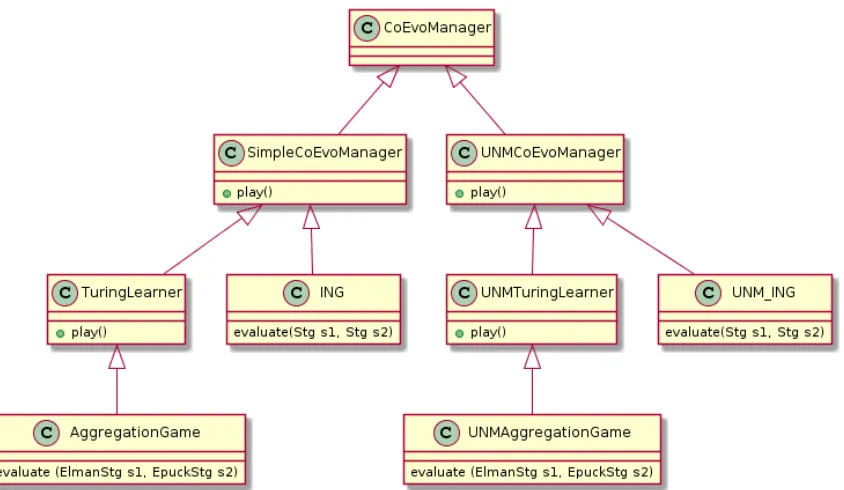
Figure 5.5: The architecture of ING and PNG game manager.

Similarly, a coevolution manager class takes the type of players and their strategies as parameter. Games using the same solution concept and architecture can reuse the code of the coevolution manager (e.g., the ING and PNG game; see Figure 5.5). In the following example, the code of

SimpleCoEvoManager is reused. In fact, apart from output functions, the only function to be

uniquely defined between classes is theevaluatefunction.

c l a s s ING : p u b l i c SimpleCoEvoManager < I n t V e c t o r S t r a t e g y , I n t V e c t o r S t r a t e g y , I N G P l a y e r , I N G P l a y e r >{}

c l a s s PNG : p u b l i c SimpleCoEvoManager < P c t V e c t o r S t r a t e g y , P c t V e c t o r S t r a t e g y , PNGPlayer , PNGPlayer >{}

5.2 Implementation 49

Figure 5.6: The architecture of Turing Learner.

1. Realize theEpuckStrategyclass.

2. Realize theEpuckAgentclass withEpuckStrategyas a type parameter. 3. Realize the EpuckAnimal class for real agents1.

4. Generate some replica agents according to strategy and run simulations on Enki. Record the linear and angular velocity of some agents for later.

5. Realize theElmanStrategyclass.

6. Realize theElmanNNclass withElmanStrategyas a type parameter for neural networks. 7. Take the data from previous steps and perform classification (regardless of the accuracy at this

stage).

8. Implement the model player and classifier player regarding solution concepts. 9. Implement Turing Learner classes regarding solution concepts.

10. Implement the interaction with external game solvers. 11. Realize output functions and write scripts for testing. 12. Evaluate regarding differnt parameters.

This project first performs an examination of the hard-coded implementation from [19]. Not all parameters are taken the same as that of the original work. In both implementation, the maximum speed of epuck robot is 12.8cm/s. Different from the original work, in this implementation, we bound the velocity between -1 and 1 (inclusive) so the robots not misbehave totally out of order. In fact, this can be problematic in interaction. We will discuss this in Chapter 6 As for the mutation step, we take a scale parametersc=0.4. This way, it is less probable that the new valueσ_i00is beyond the range in the second step (see Section 2.4.2 for the complete mutation):

σ_i00:=sc∗σ_i00∗exp(τ0∗r+τ∗ri),i=1, . . . ,n; (5.1) g00_i := (g00_i +σ_i00∗ri),i=1, . . . ,n (5.2)

A significant drawback of the original work is taking only R=1 replica in each simulation. We takeR=A=5 in our implementation to make the fitness values more accurate and benefit the accuracy of UNM. Another problem is the imbalance of population regarding the size of genes in the original work. There are 4 genes for a strategy of the model player while there are 92 genes for each strategy of the classifier player. In the original work, there are 50 strategies managed by each player and they reproduce 50 offspring each. For the model player, each gene shares 50/4=12.5 offspring. In contrast, for the classifier player, each gene shares at little as 50/92=0.54, over 20 times less than that of the model player. In this project, we let the classifier reproduce 100 offspring instead2. Further discussion is included in Section 6.1. In addition, we taker0=8 andr1=10 to

help the update of population of the classifier player.

5.3 Evaluation

5.3.1 The PNG and RNG Game

This project takes the ING game as a cases study for the correctness of implementation (Section 4.4). Similarly, the PNG and RNG games are introduced as test cases for a quantitative measurement on how UNM would speed up the convergence regarding different correlated populations. We introducedε as a coefficient in Section 3.3 in the evaluation function. The largerε is, the more attractive the point of an opponent strategy in comparison with the pre-defined attractor (as a point in 2D space) and thus harder to converge to the attractor. We show the difference between a naive coevolutionary process and that using UNM. Whenε<1, the two populations converge and settle at the pre-defined attractors respectively (Figure 5.7). Otherwise the population may settle at a point in between (see Figure 5.8). It is clear from the figure that there are significantly less strategies explored in the space when using UNM3.

We further examine the impact ofε on coevolution for PNG and RNG games respectively. We take two points in 4D space: p1={0.2,0.2,0.2,0.2}andp2={0.8,0.8,0.8,0.8}as attractors. For

the PNG game, Figure 5.11 shows that a largerεmakes the entanglement more significant and thus harder for the population to converge. However Figure 5.12 shows that for RNG game, this impact is not as significant. In both cases, the use of UNM can significantly boost convergence but slow down the computation due to the calls to the external solver. Different from the ING game, there

2_{This is still far from “enough” to be balanced, considering the combination of all the values of each gene.}

5.3 Evaluation 51

Figure 5.7: RNG withε=0.2. Figure 5.8: RNG withε =2.

(a) coevolution withε=0.2)

(b) coevolution withε=0.8