A Tangential Microslip Model for Circularly and Elliptically Loaded Structures

This is a repository copy of A Tangential Microslip Model for Circularly and Elliptically

Loaded Structures.

White Rose Research Online URL for this paper:

http://eprints.whiterose.ac.uk/97156/

Version: Accepted Version

Article:

Lord, C.E. orcid.org/0000-0002-2470-098X and Rongong, J.A.

orcid.org/0000-0002-6252-6230 (2016) A Tangential Microslip Model for Circularly and

Elliptically Loaded Structures. Proceedings of the Institution of Mechanical Engineers, Part

C: Journal of Mechanical Engineering Science , 230 (6). pp. 900-909. ISSN 0954-4062

https://doi.org/10.1177/0954406215608409

Reuse

Unless indicated otherwise, fulltext items are protected by copyright with all rights reserved. The copyright exception in section 29 of the Copyright, Designs and Patents Act 1988 allows the making of a single copy solely for the purpose of non-commercial research or private study within the limits of fair dealing. The publisher or other rights-holder may allow further reproduction and re-use of this version - refer to the White Rose Research Online record for this item. Where records identify the publisher as the copyright holder, users can verify any specific terms of use on the publisher’s website.

Takedown

Original Article

A tangential microslip model for circularly and elliptically

loaded structures

Charles E Lord and Jem A Rongong

Department of Mechanical Engineering, Dynamics Research Group,

University of Sheffield, Sheffield, S1 3JD, United Kingdom

Email: [email protected]

Abstract

It is well known that the noise and vibration control of structures is a continuing challenge. With many

structures this is commonly achieved through passive vibration damping; often using viscoelastic

materials. It is sometimes however that the use of such materials is not permitted as their properties

change over time, or when they are subjected to low and high temperature environments. For these

structures and structural elements, it is often that clamping or applied boundary conditions are critical

for providing the energy dissipation through microslip. This makes it necessary to understand the level of

damping that arises from the clamping zones. In general, the estimation of damping is complicated in that

most structures are not uni-directionally loaded and can have a planar path of motion (e.g. gas turbine

blades, circular motion valves). Although it is typical during experiments and simulations to reduce a

structure into a single axis of excitation, this can often be an over simplification which does not describe

the dynamics of the system; but should be included. This paper presents a biaxial planar motion

tangential microslip model that accounts for the vibratory loads arising from circular and elliptical

motion. This model vectorially decouples and reduces the planar vibratory circular and elliptical motion

into two separate independent tangential microslip models. The models account for tip loading and for

centroid loading within the microslip region of the clamping zone. Each analytical microslip model is

presented and is compared to numerical simulations using finite elements. The analytical models are then

Original Article

within the structure. The coupled models are then compared to numerical simulations using finite

elements through ANSYS.

Keywords

Friction model, microslip, damping, hysteresis

1 Introduction

Typically, clamped joints express two different types of motion during vibrations: microslip and

macroslip. When a tangential force is applied to a clamped joint small zones at the clamp initially break

free and allow slipping to occur in localised areas; this is referred to as microslip. If the force is large

enough, the microslip will propagate throughout the entire clamped joint and will result in gross slip; this

is known as macroslip. In this paper, macroslip is not considered but rather focus is confined to purely

microslip and therefore various friction models and stick-slip behaviour are not discussed.

Vibrational damping in most structures, without purpose-driven damping elements, is relatively

small. This is especially true with metallic structures. The joints within these structures serve as a method

that can be instigated for increasing the level of damping. For example, work done by Hartwigsen et al [1]

has demonstrated experimentally the nonlinear effects from a beam with a shear lap joint. They showed

that damping ratios could be greater than 0.03 depending on the exciting amplitude.

Although the use of joints as a method of promoting damping is not a new approach, there is still

inadequate knowledge of how to model the behaviour of these structures accurately and, all importantly,

how to design efficient structures utilising them. It is however well-recognised that the dynamic response

of clamped joints is strongly affected by microslip. For these reasons further understanding is a necessity.

Original Article

parallel-series model. They showed that with the correctly chosen parameters, their model predicted

energy dissipation and matched experimentally obtained responses for a range of excitation frequencies

and amplitudes. Following this work, Cigeroglu et al [4] proposed a similar model, differences being that

this model included the inertia from the bar and that the normal force was non-uniform. They

demonstrated that as the excitation frequency approached the natural frequency that the system began to

soften. Using the Fourier coefficients, they then developed a point friction model. Xiao et al [5] studied

the energy dissipation of a mechanical lap joint using the one-dimensional friction model developed by

Menq et al [2]. They were interested in the contact interface tangential stiffness and pressure distribution

laws on the energy dissipation at bolted joints. They demonstrated that as the pressure law coefficient

increased, the stiffness decreased and as the elastic stiffness of the shear layer decreased that the

hysteresis loops began to resemble a viscoelastic response. Sanliturk and Ewins [6] modelled the

two-dimensional behaviour of a point friction contact using the harmonic balance method. Their proposed

efforts were an extension of work from Menq et al [7]. One of the main differences from others is that in

their model they were not limited to Coulomb friction while the friction force at the joint was

accommodating to either experimental or theoretical data.

In this paper a two-dimensional clamped joint is considered that is exposed to circular and

elliptical loading. Clamping with preload is applied on three sides around the perimeter of the clamp

(detailed in Figure 2). A sinusoidal forcing function is applied for each direction (orthogonal) at the same

frequency with a zero phase shift. This forcing function originates from the portion of the cantilever

structure that extends beyond the clamped zone creating the tangential loading. The harmonic loading is

considered to be small compared to the clamping preload force and therefore the coupling of the

Original Article

2 Mathematical model

The planar tangential model presented in this paper is coupled by two different and distinctive

one-dimensional tangential models: tip loading and centre loading. The tip and centre loading are defined as

axial loadings applied to the biased extreme boundary and applied to the centroid of a 2-D bar,

respectively. Each of the tip loaded and centre loaded models are based on a backward finite difference

approach to find the force-displacement response. The loads at the clamping zone originate from the

inertial loads external to the clamping zone. The circular and elliptical motion is created depending on

 

 

T tip

T centre

F R

F

 , (1)

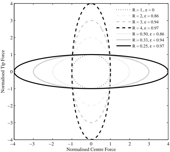
where FT is the force being applied to the contact zone. The two-dimensional trajectories being

considered are listed in Figure 1.

−4 −3 −2 −1 0 1 2 3 4

−4 −3 −2 −1 0 1 2 3 4

Normalised Centre Force

Normalised Tip Force

R = 1., ε = 0 R = 2, ε = 0.86 R = 3, ε = 0.94 R = 4, ε = 0.97 R = 0.50, ε = 0.86 R = 0.33, ε = 0.94 R = 0.25, ε = 0.97

Original Article

Both the tip and centre loaded models ignore the clamped zone mass making the assumption that the

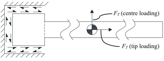
external mass (or equivalent mass) is significantly larger. An example of this type of loading is shown in

Figure 2.

Figure 2: Two-dimensional tip and centre loading on clamping zone

The mass external to the clamped zone is assumed to act as a translational moving rigid body in both the

tip and centre loading directions ignoring any bending. Shear deformations for the mass inside the

clamped zone are ignored as they are relatively minute in amplitude.

For each simulation the preload (normal force) and coefficient of friction are considered to be

constant. Furthermore, the static and dynamic friction coefficients are equal and any transition is

neglected.

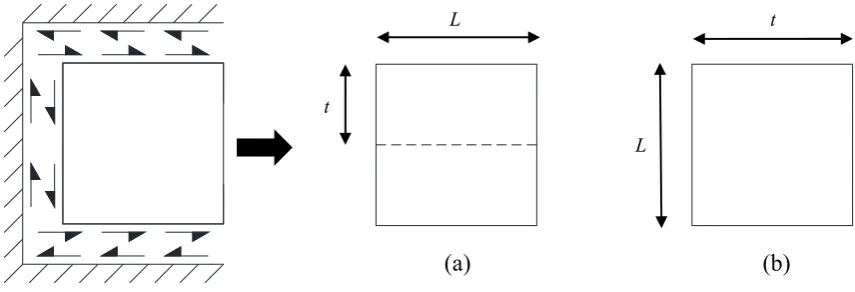
Since the loading for each of the models is perpendicular to the other, the notation of the geometric

variables for the length, L, and thickness, t, requires a slight alteration. This is depicted in Figure 3.

Considering the clamped zone from Figure 2, when applying the tip loading, the clamped zone has a line

of symmetry. Therefore the two symmetric halves act in parallel and only one half needs to be considered

(each half accepts half of the tip force). Converse to this, the centre loading does not contain a line of

symmetry so the entire clamped zone needs to be evaluated.

FT (centre loading)

Original Article

Figure 3: Clamped zone orientation for length, L, and thickness, t, for (a) tip loading and (b) centre loading

Since a symmetric loading is being used, both models will only include the first loading cycle and the

completion of the force-displacement hysteresis loop will be achieved using Masing’s Rule [8] in this

paper.

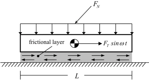
2.1 Tip loading

The motion caused from the tip loading for the mass in the clamped zone is such that the microslip begins

at the edge that is closest to the external mass. The tip loaded microslip model is such that a uniformly

distributed clamping load, FN, is placed on the non-stationary part. The microslip model assumes that the

interface always being in full contact over the entire surface and that no overlap is permitted. Unlike

microslip from bending, under axial tip loading, the microslip begins at the inception of the applied tip

force meaning that no fully sticking contact condition exists. For the first phase, the microslip model is

initiated by applying the load from the external mass, FT, incrementally. The chosen increment size of FT

is important for defining the shape of the hysteresis loop as it relies on a back-looking approach of the

displacement of the previous increment of FT. A graphical representation of the model is shown in Figure

(a)

(b)

L t

t

Original Article

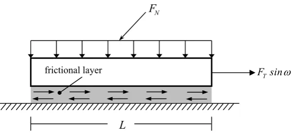
Figure 4: One-dimensional tip loaded axial microslip model

Since FT is applied perpendicular to FN, and FN is distributed over the length of the layer, FN can then be

expressed as a distributed loading along the length such that,

N

F q

L

 , (2)

where L is the length of the clamp zone in Figure 3 and  is the friction coefficient. Equation 1 implies

that for any increment of FT applied, some amount of slip will immediately be returned. The slip zone for

the first iteration is then described by

 1

1

T i i

F u

q



  . (3)

When applying FN, slipping begins at the edges of the contact area and progresses toward the centre as FN

increases. This slipping is however ignored and is considered to be negligible. Substituting Equation 2

into Equation 3, the slip zone length for the subsequent iterations is expressed as

L

N

F

T

F sin



Original Article

 





T i x i

i N F L u F  

 , (4)

where x is the axial displacement that is used to update L and the subscript i denotes the increment of FT .

It becomes apparent that macroslipping is initiated once

T N

F



F

Poisson’s ratio effects have been included for both the tip and centre microslip models since a no sticking

condition is achieved and that the compressive loads could be rather high resulting in high FT under

displacement controlled excitation. Although the volumetric change from Poisson’s ratio occurs evenly

for each direction, one key assumption that is made is that in the thickness direction, the thickness

changes are accumulated only in a single direction. Meaning that any increase and/or decrease in

thickness occurs at the top surface of the sample only so that contact is maintained at all times. The depth

and thickness are respectively expressed as

 

1 1

1 1 i T i

i i i i w F w w Ew t        _ _

 , (6)

and

 

1 1

1 1 i T i

i i i i t F t t Ew t           

Original Article

where is Poisson’s ratio and E is the modulus of elasticity. Once slipping occurs, the friction is fully

overcome and the interface behaves as though it is frictionless where slipping is present for the amplitude

of force that is being applied that exceeds the friction force. Knowing that the axial stiffness of a uniform

cross-section is defined as

AE k

L

 , (8)

where A is the cross-sectional area, substituting Equations 4, 6 and 7 into Equation 8, the axial stiffness of

the portion of the bar that is slipping becomes

2

i i i

i

w t E

k u

 . (9)

The stiffness in this case is doubled as not only does the slipping have to be overcome but also a load that

is necessary to allow for displacement of the slipped zone. Although the microslip resembles a

nonlinearity, each displacement is linear. Therefore, the displacement is expressed by

  T i 

x i i

F k

 . (10)

2.2 Centre loading

Converse to that from the tip loading, the motion created by the centre loading, for the mass located

within the clamped zone, is such that the microslip originates at the centre. The non-stationary sample of

Original Article

preload. The microslip model is predicated on the interface always being in full contact over the entire

surface and that no overlap exists between the sample and the constrained support. Unlike microslip from

bending, and similar to axial tip loading, the microslip begins at the inception of the applied centre force

resulting in a non-fully sticking contact condition. For the first phase, the microslip model is initiated by

applying the load from the external mass, FT, incrementally. The resolution and accuracy for the shape of

the hysteresis loop is defined by the chosen increment size of FT as it relies on a back-looking approach of

the displacement of the previous increment of FT. A graphical representation of the model is shown in

Figure 5.

Figure 5: One-dimensional centre loaded axial microslip model

Like the tip loaded microslip model, the same assumptions apply and too when FN is placed on the

non-stationary sample, the microslip caused from it is considered to be negligible and is therefore omitted.

Microslip begins when FT > 0, however this now originates at the centre of the sample. Unlike that of the

tip loaded microslip model, where the tension and compression occur separately, the compression and

tension for the centre loaded microslip model occurs simultaneously for each phase. Consequently, to

determine the hysteresis loop, the sample is split at the centre of mass along the length separating the

tension and compression domains. Knowing that the slip zone develops from Equation 3 and that FT is

L

N

F

T

F sin



Original Article

equally shared between the tension and compression domains, the slip zone of interest for each domain

for the first phase is defined as

 





4

T i x ic ,it ic ,it

N

F L

u

F

 



 , (11)

where the subscripts ic and it define the increment for the compression and tension domains, respectively.

For the first increment, x(ic−1,it−1) = 0 and the slip zones are equal to one another. Since both tension and

compression occur simultaneously, a reduction and an increase in cross-sectional areas occur at once but

at different rates. Hence, the Poisson’s ratio effects need to be computed for each domain separately. The

depth and thickness changes for the compression domain are increasing in cross-sectional area and are

expressed as

 1

1

x ic ic

ic

w

w w

u





  , (12)

and

 1

1

x ic ic

ic

t

t t

u





  . (13)

On the other hand, the tension domain is reducing in cross-sectional area so the depth and thickness

Original Article

 1

1 x it it it w w w u  

  , (14)

and

 1

1 x it it it t t t u  

  . (15)

Now that the Poisson’s ratio effects have been included, the stiffness shift for each domain is expressed as

2

ic ,it ic ,it ic ,it

ic ,it

w t E

k

u

 . (16)

Following the same format as Equation 10, the displacement for the compression and tension domains are

expressed as

  T ic,it 

x ic,it

ic,it

F k

 . (17)

Up to now, the peak displacements that have been computed are related to the restriction of no

participation from the other domain. The total peak centre displacement of the system is now expressed as

a combination of the peak displacements for each of the domains and is given as

 









ic x ic it x it

x i ic it k k k k  

Original Article

3 Model coupling

To find the overall damping from the two models, for the planar motion in the clamping zone, a coupling

between the models is required. In the approach that is listed in this paper, the hysteresis loops for each of

the different loadings (tip and centre) are required which are defined from above in the previous sections.

The coupling is achieved by vectorially combining the two independent motions to create a resultant

hysteresis loop as shown in Figure 6. For clarity, the solid lines indicate the data located in the

positive-positive-positive quadrant while the dashed lines are for data in all other quadrants.

Figure 6: Euclidean space representation for resultant hysteresis loop. For clarity, solid lines indicate the positive-positive-positive octant data and dashed lines represent the remaining octants data.

Once the hysteresis loop for each model is established, the resultant hysteresis displacement can be

defined by

tip centre

FT

Resultant hysteresis loop

Original Article

       

 

2 2 x it

x ir x it x ic

x it       _{ }    

, (19)

where the subscript ir denotes the resultant iteration. In a similar approach, the resultant hysteresis force

can also be described by

       

 

2 2 T it

T ir T it T ic

T it

F

F F F

F       _{ }    

. (20)

Once the resultant displacement and force are both found, the resultant hysteresis can then be formed.

Using the resultant hysteresis loop, the total absorbed energy, Wd, and peak strain energy, U, can be

estimated and is accomplished by

Wd 





and             0

x ir T ir

x ir T ir ,F

T ir x ir ,F

U F









where is the peak amplitude. By knowing Eqs. 20 and 21, the damping loss factor is then conventionally

Original Article

2

d

W U

 . (23)

4 Finite element model

ANSYS commercial finite element (FE) code is used as the FE solver. The FE model employs 3-D solid

higher-order hexahedron (SOLID186) and 2-D contact elements with approximately 10500 degrees of

freedom. Only two different parts are needed for the FE model: a base and a sample. The sample

represents the mass that is inside the clamping zone while the base represents the rigid clamp. Contact

pairs consisting of contact (CONTA174) and target (TARGE170) elements are used to provide interaction

between the mass and clamped zone through the implementation of Coulomb friction. The interpretation

of Coulomb friction for ANSYS is that the product of the force normal to the sliding direction and the

friction coefficient is a limiting force. If the tangential force is less than the limiting force the state of the

contact is sticking. However, if the tangential force is equal or greater than the limiting force then the

contact is sliding producing relative motion. An augmented Lagrange contact formulation is used to help

with convergence. This method is an iterative series whereby the pressure and frictional stresses are

augmented during the equilibrium iterations resulting in the final contact penetration being decreased and

lower than the user-defined allowable penetration. This generally leads to better conditioning of the

stiffness matrix as compared to other penalty methods. A contact stiffness factor of 1, which is updated

for each equilibrium iteration, is used to minimise the amount of penetration between the sample and

base. Although the sample is not subjected to large deflections, nonlinear geometry is accounted for to

accommodate the sliding of the contact elements. The FE model configuration is shown in Figure 7.

FN

Original Article

Figure 7: Example FE model for the mass and clamp zone

A single loadstep was used for each simulation comprised of a sinusoidal load applied over a

duration equal to 125% of the frequency period (1Hz was used in this paper). The first 25% of the period

moves the sample from rest into the hysteresis loop path while the remaining 100% of the period

completes a loop. To help with convergence further, and to gain meaningful and comparable results with

the tip and centre loaded models, the tip and centre loads were discretised into 50 linearly-spaced

substeps. The size of the substeps is dependent on several factors (e.g. mesh, deformation). However,

possibly the most important of them being the contact element mesh density. The mesh density needs to

be sufficient to capture the stick-slip of the contact region. Each substep was then split into a maximum of

26 equilibrium iterations while outputting the Newton-Raphson residuals for convergence checking.

As also noted in the tip model, when the tip force is initiated, the contact zone of the tip breaks

free firstly while propagating to the root end of the sample. In a similar way, when the centre load is

firstly applied to the centre model, the centre contact zone of the sample commences slipping and extends

toward the edges as the load increases. The slip growth for the various loading and unloading phases is

illustrated in Figure 8.

F

compression

F

tension/compression

Original Article

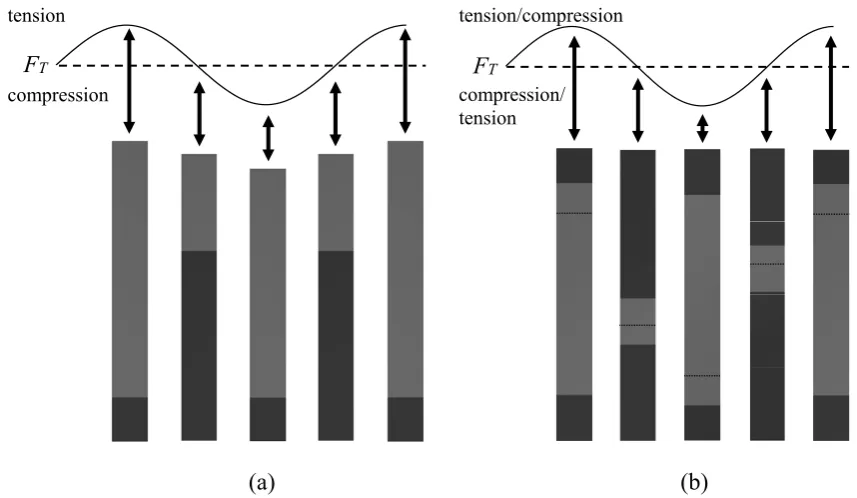
Figure 8: Typical contact status and exaggerated deformations from FE simulation for various loading and unloading phases for (a) tip loading and (b) centre loading

Figure 8 shows the sticking (dark grey) and slipping (light grey) regions at the end of each 90° for the

sequential tip and centre harmonic loading. For the tip loading, the bottom-most portion is constrained

while the top-most portion is where FT is applied. It is clear that when tension loading the portion of the

layer that is slipping is elongated and that as the slip zone decreases, the stiffness is increased and that the

elongation is reduced. For the centre loading, the black lines indicate the displaced position of L/2. It is

clear that unlike the tip loading, the overall length of the layer remains constant since the loading is

confined to the microslip region and is in the centre.

5 Results and discussion

A total of seven unique loading eccentricities were used as depicted in Figure 1. To validate the accuracy

and propriety of the mathematical models, numerical models using FEs are used as a comparison. For the

ease and interest of reducing computational time, for the nonlinear simulations, the comparisons are made

using a simplified geometry. The geometry, material properties and parameters used for the simulations

Original Article

L

(mm)

w

(mm)

t

(mm)

E

(MPa)

_F

_(N)

_F

_(N)

254

25.4

3.18

68947

0.3

0.8

445

267

Table 1: Simplified geometry, properties and parameters

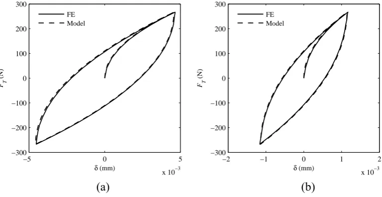
Although this geometry has been simplified, it still contains all of the important aspects of the actual

clamped joint. The comparison between the mathematical model and numerical model, for the tip loading

and centre loading, are given in Figure 9a-b, respectively. To balance the accuracy of the FE model and

the computational time, the contact mesh adequacy was defined in these simulations as a difference in

contact sliding distance as less than 0.5%.

−5 0 5

x 10−3 −300

−200 −100 0 100 200 300

δ (mm)

FT

(N)

FE Model

−2 −1 0 1 2

x 10−3 −300

−200 −100 0 100 200 300

δ (mm)

FT

(N)

FE Model

Figure 9: FE and mathematical model comparison for (a) tip loading and (b) centre loading

For the example joint that is used in this paper, for the comparison of various eccentricities for the

mathematical models, the joint geometry along with the properties and parameters are identified in Table

2. The amplitude of FT that is applied to the tip model is 2000N, 4000N, 6000N and 8000N and for the

Original Article

centre model 4000N, 8000N, 12000N and 16000N. The FT for the tip model is half that of the centre

model since symmetry is being used.

model

L

(mm)

w

(mm)

t

(mm)

E

(MPa)

_F

_(N)

tip

50

10

25

10000

0.3

0.8

20000

centre

50

10

50

10000

0.3

0.8

20000

Table 2: Respective joint geometries, properties and parameters

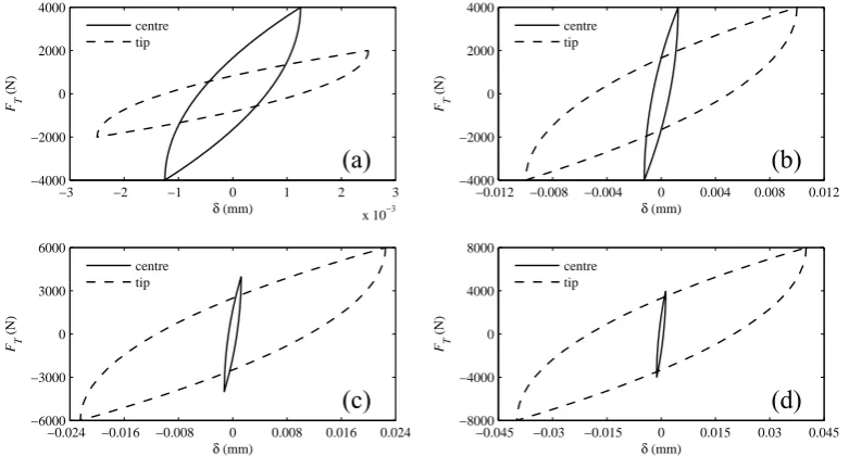
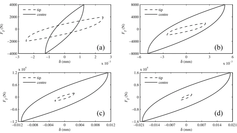
The results for each of the circular and elliptical force ratios and eccentricities, defined from Figure 1, are

shown in Figures 10 (R=1, 2, 3 and 4) and 11 (R=1, 0.50, 0.33, 0.25). It is noticed that as FT is increased

for each of the models, the stiffness decreases having a softening effect. It is also obvious from Figure 8a

that the stiffness of the centre model is greater than that of the tip model.

−3 −2 −1 0 1 2 3

x 10−3 −4000

−2000 0 2000 4000

δ (mm)

FT

(N)

−0.012 −0.008 −0.004 0 0.004 0.008 0.012 −4000

−2000 0 2000 4000

δ (mm)

FT

(N)

−0.024 −0.016 −0.008 0 0.008 0.016 0.024 −6000

−3000 0 3000 6000

δ (mm)

FT

(N)

−0.045 −0.03 −0.015 0 0.015 0.03 0.045 −8000

−4000 0 4000 8000

δ (mm)

FT (N) centre tip centre tip centre tip centre tip

Figure 10: Tip and centre loading force-displacement hysteresis loops for (a) R=1, =0, (b) R=2, =0.86, (c) R=3, =0.94 and (d) R=4, =0.97

(a) (b)

Original Article

−3 −2 −1 0 1 2 3

x 10−3 −4000

−2000 0 2000 4000

δ (mm)

FT

(N)

−6 −3 0 3 6

x 10−3 −8000

−4000 0 4000 8000

δ (mm)

FT

(N)

−0.012 −0.008 −0.004 0 0.004 0.008 0.012 −1.2

−0.6 0 0.6 1.2x 10

4

δ (mm)

FT

(N)

−0.021 −0.014 −0.007 0 0.007 0.014 0.021 −1.6

−0.8 0 0.8 1.6x 10

4

δ (mm)

FT (N) tip centre tip centre tip centre tip centre

Figure 11: Tip and centre loading force-displacement hysteresis loops for (a) R=1, =0, (b) R=0.5, =0.86, (c) R=0.33, =0.94 and (d) R=0.25, =0.97

The normalised vibration damping loss factor for the different forcing ratios (eccentricities) is shown in

Figure 12. Interestingly the highest damping loss factors are at the extreme elliptical motion. This is

directly associated with the combination of the ellipticity and the increase in FT. This information follows

the findings by Hartwigsen et al [1].

(a) (b)

Original Article

F

T (centre)

F

tip)

1 1.5 2 2.5 3 3.5 4

1 1.5 2 2.5 3 3.5 4

normalised damping loss factor,

η

0.55 0.6 0.65 0.7 0.75 0.8 0.85 0.9 0.95 1

Figure 12: Normalised damping loss factor for various R

It is noticed from Figure 12 that when R=1, the loss factor is the lowest. Conversely, when R is minimum

and maximum (R=0.25 and R=4), the loss factor is the largest. Additionally, the gradient of the slope

between for the damping loss factor changes as R increases and decreases pivoting around R=1.

6 Conclusions

Two different tangential microslip models (tip and centre loaded) have been presented. Each model is

capable of producing force-displacement responses. Both models are compared to FE models and have

Original Article

two microslip models are combined to demonstrate the overall response for the normalised damping loss

factor for various two-dimensional trajectories

Acknowledgements

This research received no specific grant from any funding agency in the public, commercial, or

not-for-profit sectors.

References

[1] Hartwigsen, C.J.; Song, Y.; McFarland, D.M.; Bergman, L.A.; Vakakis, A.F.. Experimental study of

non-linear effects in a typical shear lap joint configuration, Journal of Sound and Vibration, 2004,

277, 327-351.

[2] Menq, C.H.; Bielak, J.; Griffin, J.H. The influence of microslip on vibratory response, part I: A new

microslip model, Journal of Sound and Vibration, 1986, 107(2), 279-293.

[3] Menq, C.H.; Griffin, J.H.; Bielak, J. The influence of microslip on vibratory response, part II: A

comparison with experimental results, Journal of Sound and Vibration, 1986, 107(2), 295-307.

[4] Cigeroglu, E.; Lu, W.; Menq, C.H. One-dimensional dynamic microslip friction model, Journal of

Sound and Vibration, 2006, 292, 881-898.

[5] Xiao, H.; Shao, Y.; Xu, J. Investigation into the energy dissipation of a lap joint using the

one-dimensional microslip friction model, European Journal of Mechanics A/Solids, 2014, 43, 1-8.

[6] Sanliturk, K.Y.; Ewins; D.J. Modelling two-dimensional friction contact and its application using

harmonic balance method, Journal of Sound and Vibration, 1996, 193(2), 511-523.

[7] Menq, C.H.; Chidamparam, P.; Griffin, J.H. Friction damping of two-dimensional motion and its

Original Article

[8] G. Masing. Eigenspannungen un verfestigung beim messing. Second International Congress for