Towards universal quantum
computation through relativistic
motion
David Edward Bruschi
1,2, Carlos Sabín
3, Pieter Kok
4, Göran Johansson
5, Per Delsing
5&
Ivette Fuentes
1We show how to use relativistic motion to generate continuous variable Gaussian cluster states within cavity modes. Our results can be demonstrated experimentally using superconducting circuits where tuneable boundary conditions correspond to mirrors moving with velocities close to the speed of light. In particular, we propose the generation of a quadripartite square cluster state as a first example that can be readily implemented in the laboratory. Since cluster states are universal resources for universal one-way quantum computation, our results pave the way for relativistic quantum computation schemes.
Quantum technologies are expected to bring great benefits to many human endeavours in the not-too-distant future. In the past decades it was shown that devices exploiting the laws of quantum mechanics can in principle cross boundaries that classical devices cannot. Advanced systems such as quantum memories and quantum com-puters are being developed in an effort to realise these transformative quantum technologies1. In addition to the
practical aspects of quantum technologies, there is great interest in viewing quantum information processing as a fundamental description of Nature. This leads naturally to the question of how quantum information processing is affected by relativistic motion2. Here, we ask the question of how the relativistic motion of a cavity mirror can be
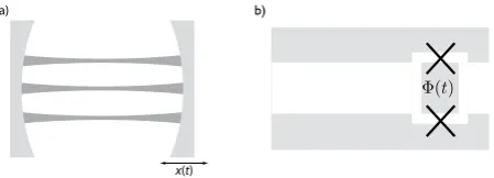
used to achieve a quantum state inside the cavity that can in principle be used for quantum computation. We show that we can create such a universal resource state in the continuous variables defined by the quadratures of the field modes inside the cavity. This proposal can be implemented practically using superconducting circuits (see Fig. 1). Recently, it was shown that relativistic motion can be used to generate bipartite quantum gates. In particu-lar, two-mode squeezing3 and beam-splitting gates4 between field modes were implemented through the non-
uniform acceleration of a cavity. A promising experimental realisation of these scenarios is circuit Quantum Electrodynamics (cQED), where Superconducting Quantum Interferometric Devices (SQUIDs) provide tuneable boundary conditions corresponding to mirrors moving at speeds close to the speed of light in the medium. This possibility was exploited for the first experimental observation of the Dynamical Casimir Effect, i.e., particle creation through relativistic motion of boundary conditions5,6. We note that the beam-splitting gate was recently
experimentally demonstrated in this type of system7 and that two-mode squeezing involving two distinct cavity
modes has also been achieved in cQED8. Moreover, some of us have shown that the same phenomenon originates
an observable effect in the fidelity of quantum teleportation between two superconducting cavities, one of them undergoing a temporal variation of the boundary conditions9. These works open a new avenue of research on the
effects of relativistic motion and gravity in generic quantum technologies, and in particular quantum computing with continuous quantum variables. While it is possible to transfer the continuous-variables entanglement gener-ated in the Dynamical Casimir Effect to discrete-variables systems such as qubits10 the analysis of relativistic effects
in qubits is typically limited by the impossibility of achieving relativistic velocities -which can only be accessed in a quantum simulator11.
Quantum computation with continuous variables (CV) has attracted a great deal of attention as an alternative to the traditional qubit approach to quantum computing12, and the CV version of measurement-based quantum
computing is well-developed13–16. In this paradigm for quantum computing the quantum gates are implemented by
1School of Mathematical Sciences, University of Nottingham, University Park, Nottingham NG7 2RD, United Kingdom. 2School of Electronic and Electrical Engineering, University of Leeds, Woodhouse Lane, Leeds, LS2 9JT, United Kingdom. 3Instituto de Física Fundamental, CSIC, Serrano 113-bis, 28006 Madrid, Spain. 4Department of Physics & Astronomy, University of Sheffield, Sheffield S3 7RH, United Kingdom. 5Microtechnology and Nanoscience, MC2, Chalmers University of Technology, S-41296 Göteborg, Sweden. Correspondence and requests for materials should be addressed to C.S. (email: [email protected])
measurements on a particular type of multipartite entangled state known as a cluster state. Assuming that we can implement the required measurements (via homodyne detection and photon counting17), these states are universal
for quantum computation. A practical way to create CV cluster states in a cavity using non-relativistic methods is by creating an entangled optical frequency comb18, a proof-of-principle experiment of which was recently performed19.
In this paper we show how to generate large CV regular cluster states through the relativistic accelerated motion of a cavity. The quantum field inside the cavity is initially in the vacuum state. We exploit entanglement resonances among different modes of the cavity3 to show that, by suitably choosing the motion of the boundaries, it is possible
to generate specific multimode entangled states. These states can always be transformed into regular CV cluster states by suitably phase-shifting some of the modes. We propose a specific implementation with superconducting cavities in which the motion of the boundary conditions is implemented through tunable SQUIDs. In particular, we show an example with four modes that is within reach of current technology. In this way, we also contribute to transferring the concept of measurement based quantum information processing using continuous variables to the field of cQED.
In the Methods section we will review the technical tools required to describe quantum fields in relativistically moving cavities. In the Results section we show how to produce CV cluster states using relativistic motion and we present an experimental implementation in superconducting circuits. We conclude our paper with a discussion of our results.
Methods
Technical tools: quantum fields confined within moving cavities.
In this section we review the technical tools to describe relativistic quantum fields, following mainly ref. 3 unless stated otherwise. We consider that the length of the cavity is constant in the reference frame of an observer co-moving with the cavity. Using the covariance matrix formalism, we show how to use entanglement resonances to create a two-mode squeezing gate in the case the motion is either discrete or continuous. Finally, we show that the gates can also be produced in case a single cavity wall oscillates.Field quantization within a cavity. We consider a massless field Φ confined within a 1 + 1 cavity in flat space-time, which can be employed to model a single polarisation-mode of light20. We use Minkowski coordinates ( , )t x which
are a convenient choice to describe the field when the cavity undergoes inertial motion (in this work the signature is (− , + )). The left and right boundaries of the cavity are initially at positions xL and xR respectively, where xL<xR, the length of the cavity is L := xR−xL and we impose Dirichlet boundary conditions at the walls of the cavity, i.e.
Φ( ,t xL) = Φ( ,t xR) =0. When the cavity is inertial, the mode solutions φn( , )t x to the Klein-Gordon equation
Φ =0 form a discrete set and take the form
φ
π
( , ) = ( ( − )),
( ) ω
− t x
k e k x x
1
2 sin 1
n
n it
n L
n
where the Minkowski frequencies are defined as ωn=c kn=πnc L/ and the modes φn( , )t x satisfy the eigenvalue equation
φ ω φ
∂ ( , ) = ( , ). ( )
i t nt x n n t x 2
The field Φ can be expanded as
∑
φ φΦ = ( , ) + ( , ) ,
( ) =
+∞
⁎ †
t x a t x a
[ ]
3
n 0 n n n n
where the operators {a an, n†} are bosonic operators which satisfy the canonical commutation relations
δ , † = a a
[ n m] nm and define the vacuum by an0 =0 for all n∈.
[image:2.595.157.382.45.126.2]We consider that at t=0 the cavity undergoes a period of uniform acceleration. Our formalism can be used to describe both discrete and continuous changes in acceleration. Rindler coordinates ( , )η χ are a suitable choice to describe the cavity during periods of accelerated motion. The transformation between Minkowski and Rindler coordinates is given by
χ η χ η = ( ) = ( ), ( ) t c x sinh cosh 4
where χ>0 has dimensions of length and η∈ is the dimensionless Rindler time coordinate. The proper accel-eration of an observer moving along a trajectory χ= c t2 2−x2 =const is a= /c2 χ. A crucial point is that we
consider that the cavity length is constant with respect to this observer. The observer’s proper time τ is related to the Rindler time coordinate by τ=χη/c. Thus we can write t= ac sinh acτ, x= ca2 cosh acτ and
( )
τ= acarctanh ctx , as has been done in3. The solutions φ
n to the Klein-Gordon equation in Rindler coordinates
take the form
φ τ χ
π χ χ
( , ) = ( − ) ,
( ) τ
− Ω
K e K
1
2 sin[ ] 5
n
n i
n L
n
where the Rindler frequencies are defined as Ω =n cKn=n cπ /(χR−χL). The Rindler modes φn satisfy the
eigenvalue equation
φ τ χ φ τ χ
∂τ ( , ) = Ω ( , ). ( )
i n n n 6
During the periods of uniform acceleration, the field Φ can be therefore expanded in these coordinates as
∑
φ τ χ φ τ χΦ = ( , ) + ( , ) ,
( ) =
+∞
a ⁎ †a
[ ]
7
n 0 n n n n
where the annihilation operators an define the Rindler vacuum 0 by an0 =0 for all n∈ and satisfy the
canon-ical commutation relations [ a an, †n]=δnm.
Bogoliubov transformation. It is well known that the vacua 0 and 0 are different 21. This implies that an
accel-erated observer will disagree with an inertial one that the state 0 is devoid of particles. This fundamental obser-vation is at the basis of the most exciting phenomena predicted by quantum field theory in curved spacetimes—such as dynamical Casimir effect and Unruh-Hawking effect—and is also responsible for relativistic effects in Quantum Information tasks between moving observers9.
We now briefly review the techniques introduced in refs 22,23 to study quantum information in cavities under-going relativistic motion. The mode solutions to the Klein-Gordon equation in Minkowski and Rindler coordinates are related by the following Bogoliubov transformations21,
α β β α φ φ φ φ = , ( ) † ⁎ ⁎ † 8 0 0 0 0
where the coefficients of the infinite-dimensional matrices 0α and 0β are defined by
α φ φ
β φ φ
= ( , ) = ( , ) ( ) = = ⁎ 9
mn m n t mn m n t
0 0
0 0
and ( ⋅ , ⋅ ) is the conserved inner product, see Ref. 21. Therefore, the induced transformation between the bosonic operators is
( )
α β β α = − − . ( ) † † † † a a a a 10 T T 0 0 0 0The Bogoliubov coefficients 0βmn account for particle creation, while 0αmn account for mode mixing. It is possible to compute analytically the inner products in Eq. (9) by expanding the Bogoliubov coefficients in terms of a dimensionless parameter h=aL c/ 21, as was done in22, and one obtains
α α α α
β β β
= + + + ( ) = + + ( ), ( ) ( ) ( ) ( ) ( ) ( ) h h 11
mn mn mn mn mn mn mn
0 0 0 0 1 0 2 3
0 0 1 0 2 3
where the superscripts stands for the corresponding order in the perturbative expansion. Notice that the zero order coefficients α( )
mn0
0 are diagonal and can be written as 0αmn( )0 ≡G tn( )δnm.
The explicit expression of the first contributions to (11) can be found in ref. 22. The Bogoliubov coefficients
αmn
0 and 0βmn correspond to instantaneous changes between inertial and uniformly accelerated motion. A general
cavity trajectory can be described as a succession of such transformations followed by periods of free evolution during which the field modes acquire phases G tn( ) =exp(−i tωn) and Gn( ) =τ exp(− Ω )i nτ for inertial and
uniformly accelerated free evolution respectively22,23. Notice that G =G + ( ) h
and the modes of the cavity after any trajectory are related by a general Bogoliubov transformation of the form (8), where the transformation matrix is
− −
, ( )
† †
A B
B A 12
T T
the Bogoliubov matrices A and B are functions of the Minkowski-Rindler instantaneous Bogoliubov coefficients
αmn, βmn
0 0 and the phases Gn acquired during the periods of free evolution. The exact expression depends on the
travel scenario chosen22.
Covariance Matrix formalism. We use the covariance matrix formalism which is particularly convenient when one needs to apply quantum information techniques to quantum field theory23. In this formalism, which is
appli-cable to bosonic fields in Gaussian states, all the relevant information about the state is encoded in the first and second moments of the field. In particular, given a collection of N bosonic modes, we can collect the second moments in the Covariance Matrix σ defined by the elements σij= 〈X Xi j+X Xj i〉 − 〈 〉〈 〉2 X Xi j , where 〈 ⋅ 〉
denotes the expectation value with respect to the state of the field and the quadrature operators Xi are the
gener-alized position and momentum operators of the field modes. In this paper we follow the conventions used in ref. 23, where the operators for the n-th mode are given by
= ( + ) ≡ ,
= − ( − ) ≡ ,
( )
− †
†
X a a Q
X i a a P
1 2
2 13
n n n n n n n n
2 1
2
and [Q Pn, m]=iδnm.
The covariance matrix formalism enables elegant and simplified calculations and has been proven useful to define and analyze computable measures of bipartite and multipartite entanglement for Gaussian states12.
Every unitary transformation U in Hilbert space that is generated by a quadratic Hamiltonian can be represented as a symplectic matrix S in phase space. These transformations form the real symplectic group Sp N(2 , ), the group of real (2N×2 matrices that leave the symplectic form N) Ω invariant, i.e., S SΩ T=Ω, where the symplectic form takes the expression Ω=⊕in=1Ωi and
( )
Ω =
−0 11 0 .
i
The time evolution of the field, as well as the Bogoliubov transformations, can be encoded in this structure. The symplectic matrix corresponding to the Bogoliubov transformation in Eq. (8) can be written in terms of the Bogoliubov coefficients as
=
,
( )
S
14
11 12 13 21 22 23 31 32 33
where the mn are the 2 × 2 matrices which have the explicit form
=
( − ) ( + )
− ( − ) ( + )
. ( )
A B A B
A B A B
Re Im
Im Re 15
mn mn mn mn mn mn mn mn mn
The covariance matrix ∼σ after a Bogoliubov transformation is given by ∼σ=SσST. Let us assume that we are
only interested in the state of two modes k and k′ after the transformation. A great advantage of the covariance matrix formalism is that the trace operation over a mode is implemented simply by deleting the row and column corresponding to that mode. In the next subsection, we will apply this formalism to compute the transformed state of an initial vacuum of the field when the cavity undergoes motion of the boundary conditions.
Entanglement resonances and two-mode squeezer gates. When a cavity undergoes nonuniform motion, entangle-ment is created between every pair of modes3. Furthermore, the entanglement between chosen couples of modes
can be selectively enhanced by “resonances”. An entanglement resonance is a linear increase of entanglement proportional to the number of times a particular travel scenario is repeated3,4,22,24.
There are two different kinds of entanglement resonances in the system. The first is connected to particle cre-ation and leads to a two-mode squeezing gate3. Particle creation resonances have been extensively studied in the
context of the dynamical Casmir effect6. The second entanglement resonance is produced by mode mixing without
particle creation, which implements beam splitting gates4. In this work we will exploit particle creation resonances,
since the squeezing gates which can be produced by them are a useful resource for the generation of cluster states16.
π
ω ω
=
+ ′. ( )
T 2
16
k k
Here ωn is the the frequency of mode n. The 4×4 reduced covariance matrix of two oddly-separated modes
k and k′ is obtained by tracing over Eq. (14) yielding,
σ = σ σ
− −
+ ( ), ( )
∼
′ ×
×
r
r 2 h
2 17
kk z z
2 2 2 2
2
where r=0βkk′N cos θ with θ=2πk k/( + ′)k , and σz is the Pauli matrix. The matrix σkk′ corresponds to a
two-mode squeezed state with squeezing parameter r∝N h. It is possible to define an effective Hamiltonian which gives rise to such state,
σ
= , ′∼ ′ , ′ ( )
Hint Tk k kk k k 18 with k k, ′= ( ,Q P Q Pk k, k′, k′)T as defined in Eq. (13). It is possible to generate high degrees of entanglement by
increasing the number N of repetitions reaching squeezing degrees as high as (r1 2 . However, for large / ) N
second order terms in the Bogoliubov series expansion, which are proportional to N h2 2, can no longer be neglected.
These terms introduce thermal noise in the two-mode squeezed state having negative effects in the preparation of the cluster state. However, in the section “Continuous sinusoidal motion: Experimental scenario’’ we will show that a cluster state containing significant amounts of squeezing and entanglement can be generated with realistic experimental parameters.
Discrete and continuous motion.
The entanglement created at first order in h between any two modes with different quantum number after any travel scenario is proportional to the first order correction to beta coef-ficient Bkk( )1′, see ref. 23. In the case of sharp onsets and offsets of acceleration, the coefficient Bkk( )1′ is in turnpropor-tional to the inertial-to-uniformly-accelerated first order correction 0βkk( )1′:
β = ′
( + ′) ( − (− ) ) ( )
′
( ) kk + ′
k k 1 1 h 19
kk1 k k
0 3
All the above can be generalised to the case of accelerations that change continuously. In particular, if the cavity moves with a sinusoidal oscillation at a frequency ωd, then resonances appear for all the oddly separated modes that satisfy ωd=ωk+ωk′. The formalism for the case of a rigid cavity that oscillates as a whole can be found in
ref. 4. Notice that the timescale involved in the changes of acceleration must be comparable to the characteristic timescale of the cavity, i.e. τ2L c/ .
A single oscillating cavity wall. Next, we consider the case in which only one wall of the cavity is oscillating with frequency ωd=pω1, where p∈. The Bogoliubov coefficients for this case can be computed using a perturbative
expansion where now
= δL ( )
L 1 20
is the perturbation parameter. That is, we are assuming small oscillations, as in the dynamical Casimir effect experiment6. Notice that in harmonic motion, the maximum acceleration is given by a =δ ωL
max d2. Therefore, our
parameter hmax is given by
ω
= ( )
h L
c 21
max d
2 2 2
The Bogoliubov coefficients for this case are found in ref. 25. In particular, assuming that the time T of the oscillation is long enough,
ω1T1, ( )22
we find that the beta coefficients are given by
ω δ =
′ , ( )
′ ( )
′, −
B T k
k
2 23
kk1 1 k p k
where δk p k′, − is the Kronecker delta.
CV cluster states.
Cluster states are a particular type of multipartite entangled state that, together with potentially simple measurements, are universal for quantum computation26. In the case of cavities, informationcan be encoded in the cavity field modes which are quantum continuous variables (CV)13,14. In this section we
The Stabiliser Formalism for CV cluster states. A particularly powerful and efficient way to describe cluster states is via the stabiliser formalism27. In this technique, a quantum state ψ is described completely by a set of n operators Sj, called stabiliser operators, of which ψ is an eigenstate with eigenvalue + 1:
ψ = ψ , ∀ = , …, . ( )
Sj j 1 n 24
The stabiliser operators Sj generate an Abelian group of cardinality 2n. All the members of this group stabilise
ψ.
For continuous variables, the individual information carrying systems are quantum field modes or quantum harmonic oscillators. We can define the Heisenberg-Weyl operators
( ) =
− ( ) =
, ( )
ħ ħ
X q exp i qP andZ p exp i pQ 25
where q p, ∈ are the continuous variables, and Q and P the canonical position and momentum operators of the system. The stabiliser operator for a squeezed field mode j can then be written as28
= (∆) (− ∆ ),− ( )
Sj Xj Zj i 1 26
where ∆ =er is the squeezing strength, with r the squeezing parameter. The single operator S
j fully determines
the quantum state of mode j. When ∆ =1 the field mode j is in the vacuum state 0 j. The controlled-phase gate between two modes j and k is given by the operator
=
. ( )
CZjk exp i Q Qj k 27
We can formally create continuous-variable cluster states by preparing a set of modes in momentum-squeezed states with ∆j1, and applying the controlled-phase gate CZjk between all the modes that we wish to entangle.
This creates new stabiliser operators
′ = † = (∆) (∆) (− ∆ ).− ( )
Sj CZ S CZjk j jk Xj Zk Zj i 1 28
Expressing this in exponential form using Eq. (25) then leads to the stabiliser condition for cluster states
P Q
∑
〈 − 〉 → , 〈 − ⋅ 〉 → ,
( )
P A Q 0 or A 0
29
j
k jk k
where = ( , …,Q1 QM) and = ( , …,P1 PM), and A is the adjacency matrix for the cluster. However, ideal continuous-variable cluster states that satisfy Eq. (29) are unphysical, and there are various inequivalent ways to approach these states. While the generation based on the controlled-phase gates is conceptually the simplest way to generate CV cluster states, from a physical point of view the required entanglement is easier created using two-mode squeezing. We can write a two-mode squeezing operator as
=exp
(
−ξa aˆ ˆ† †+ξ⁎a aˆ ˆ)
. ( )30
jk j k j k
Using the Bloch-Messiah reduction29, a general multi-mode squeezing operator can then be constructed (up
to local phase shifts) according to
S=exp(−i tH), ( )31 where t is the interaction time and is a bilinear interaction Hamiltonian
=
∑
+ .( ) ˆ ˆ ˆ† ⁎ †ˆ
a B a a B a
32
jk j jk k j jk k
Such a Hamiltonian leads to a complex adjacency matrix for a graph state30
Z=ie−2Bi−2iB( )1 + ( ),O h2 ( )33
where we used that in our case h1. The matrix defines a undirected graph called an H-graph that approaches a CV cluster state up to local phase shifts in the mathematical limit r→ ∞. In particular a succession of commuting two-mode squeezing operations of equal squeezing parameter generates an H-graph state which is bipartite, that is, all the nodes in the graph can be split into two sets such that the two-mode squeezers only relate the elements of one set with the elements of the other. By introducing π/2 phase shifts on the elements of one set, the H-graph state is transformed into a continuous variable cluster state16. As we will see in detail in the Results section, in the
order terms of the Bogoliubov coefficients. The role of the second order deviations from the ideal scheme will be discussed in detail in the Results section. Cluster states can be diagrammatically represented by a graph in which each node corresponds to a party and the edges between nodes represent entanglement.
Results
In this section we show how to produce a CV Gaussian cluster state through motion of the cavity. In principle, arbitrarily large grids of entangled modes can be achieved. We will also discuss possible limitations.
Step one: establishing bipartite links.
We start by choosing an odd prime number p1. As we will discuss later, this choice allows for a more symmetric definition of the state. We then choose two modes k k, ′ that satisfy p= + ′k k. We then notice that the first order correction to the Bogoliubov beta coefficient Bkk( )1′ of anarbitrary trajectory is proportional to
∝ ′
( + ′) =
( − )
( ) ′
( )
B kk
k k h
k p k
p h 34
kk1 3 3
Once p is fixed, we see that Bkk( )1′ achieves a maximum for the couple of modes k= ( − )12 p 1 and k′ = ( + )21 p 1
and takes the value ′ ∼ ( ) − BkkMax 2p2 1.
In the following, we list the operations needed to create the multipartite entangled state i.e., we describe the motion of the boundaries in terms of total time of travel scenario. The cavity undergoes an arbitrary travel scenario that lasts a total proper time
= .
( )
T L
cp
2
35
1
As found in ref. 3 and explained above, all pairs of modes k k, ′ that satisfy k+ ′ =k p will have an entanglement resonance. At this early stage of the protocol we must notice that, unfortunately, the same happens also for all the couples of modes l l, ′ which satisfy l+ ′ =l qp where q∈. In fact, for any q there are combinations of l and l′
for which we obtain
π
ω ω
=
+ ′ = , ( )
T q L
cp
2 2
36
q
l l
and therefore, all these extra couples of modes also undergo an entanglement resonance. Note that q must be an odd number since pq must be odd and thus, no entanglement is generated to first order in h. We notice though that for these extra modes
∝ ( − ) ,
( ) ′
( )
B l qp l
q p h 37
ll1 3 3
which in general means that, already for q=3, the coefficient Bll( )′1 is approximatively 3% of the value of BkkMax′
(which has q= 1).
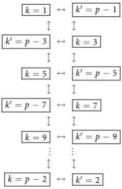
We can repeat the travel scenario any number of times in order to linearly increase the entanglement between the modes. This allows us to engineer entanglement between the following modes:
= ′ = −
= ←→ ′ = −
= − ←→ ′ = + .
( ) .
⟷
k k p
k k p
k p k p
1 1
2 2
1 2
1
2 38
ent
Here, all double arrows represent the (“large”) entanglement created between two modes. This entanglement is shown in Fig. 2 as vertical black edges.
Step two: creating a chain of entangled modes.
We next proceed to increase the entanglement links in (38), and let the cavity undergo a new travel scenario with total proper time′ =
( − ), ( )
T L
c p2 2 39
1
= ↔ ′ = −
′ = − ↔ =
= ↔ ′ = −
′ = − ↔ =
= ↔ ′ = −
( )
k k p
k p k
k k p
k p k
k k p
1 1
3 3
5 5
7 7
9 9
40 Again, the double arrows indicate entanglement, and is shown in Fig. 2 as diagonal dashed grey edges.
Step three: creating ladders of entangled modes.
Following the reasoning above, we now choose a final travel scenario with total proper time″ =
( + ). ( )
T L
c p
2
2 41
1
Once the travel scenario is repeated the necessary amount of times one achieves the multipartite state of the form
= ↔ ′ = −
′ = − ↔ =
= ↔ ′ = −
′ = − ↔ =
= ↔ ′ = −
= − ↔ ′ = ( )
k k p
k p k
k k p
k p k
k k p
k p k
1 1
3 3
5 5
7 7
9 9
2 2 42
This entanglement is shown in Fig. 2 as diagonal solid grey edges. The resulting H-graph has a ladder config-uration. The mode p itself does not participate in the graph state.
Selecting contributing entangled modes.
In the previous section we have achieved a multipartite entangled state which has the ladder structure shown in Eq. (42) and Fig. 2. We have already noted that the entan-glement between pairs of modes in Eq. (42) is not the same as quantified by Bkk( )1′. We would like to have a statewhere each entangled pair of modes exhibits the same amount of entanglement.
[image:8.595.286.406.434.619.2]Since the aim is to obtain a multipartite state with entanglement between modes that forms a particular struc-ture, we need to guarantee that the entanglement between the modes in the structure is much higher than the entanglement with other modes. For this reason, we have chosen a large prime number p1, and we keep all pairs of modes k k, ′ that satisfy
−
≥ Λ,
( ) ′
( ) ( )
( )
B B
B 43
kk1 Max1 Max1
where Λ sets a limit on the minimum amount of entanglement which we want to generate. The value of Λ sets the minimum value of k -denoted by kλp- that we consider and the corresponding number λp of mode pairs, which is
given by:
λ = − .
( ) λ
p k
2 44
p p
Notice that every time the cavity undergoes some travel scenario, λp will depend on the prime p and will be different for different sets of modes. In addition, we have chosen numbers p− , , +2p p 2. Clearly, for p1 the bounds λ , λp p−2, λp+2 will be identical given a choice of Λ. We can therefore rewrite (42) as
= − ↔ ′ = +
′ = + ↔ = −
= − ↔ ′ = +
′ = + ↔ = −
…
= ↔ ′ = ′ .
( )
λ λ
k p k p
k p k p
k p k p
k p k p
k k k k
1 2
1 2
5 2
5 2
9 2
9 2
13 2
13 2
45
p p
If λp is chosen tight enough, all modes in Eq. (45) will share almost the same amount of entanglement.
Step four: “Propagating” the entanglement.
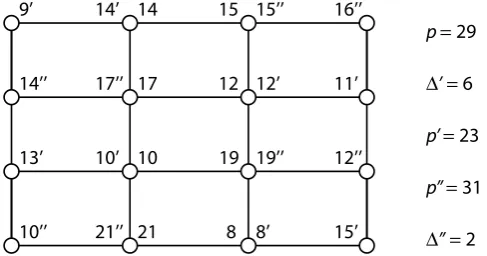
In this subsection we show how to propagate the entan-glement from the basic structure we have built in Eq. (42) and Fig. 2, to build a regular structure.Enlarging the structure of the multipartite state.
We have shown how we can create an H-graph state in which the modes are entangled according to a ladder topology (a ladder graph). We will now proceed to show how to extend the ladder graph to a square lattice graph. We choose another prime p′ >p and p= ′ − ∆′p . Since p′p would allow for substantially different amounts of entanglement, we choose a prime p′ of the same order of magnitude as p. Among the modes that will be entangled in the ladder graph generated by p there will be a mode k= ( + )21 p a that coincides with mode of k= ( ′ − )21 p b in the ladder graph generated by p′ (with , ∈ )
a b . If the mode k= ( + ) = ( ′ − )21 p a 21 p b are within the ranges defined by λp and λp′, then we can use
the travel scenari with total proper time 9’
14’’
13’
p = 29
p’ = 23
p’’ = 31
10’’
14’
17’’
10’
21’’
15
12
19
8
16’’
11’
12’’
15’ 14
17
10
21
15’’
12’
19’’
8’ ∆’’ = 2
[image:9.595.154.398.47.175.2]∆’ = 6
=
′. ( )
‴
T L
cp
2
46 Without loss of generality, we can assume that p+ = ′ − (∆′ − )1 p 1 . Therefore
where we do not specify the endpoint of the chain because it now depends on λp and λp′. We now choose another
prime p″ >p and p= ″ + ∆″p and repeat the above process to get the structure
The aim will now be to close all the links and complete the lattice of entangled modes.
Final step.
To complete our scheme, we notice that″ − (∆″ − )
+ ′ + (∆′ − ) = + ∆′ − ∆″ − ′ + (∆′ − )
+ ″ − (∆″ − ) = − ∆′ + ∆″ +
( )
p p p
p p p
1 2
5
2 2
1 2
5
2 2 49
which are both odd numbers. This again guarantees that the entanglement is created at first order in h. We now let the cavity undergo two travel scenarios with proper times
=
( + ∆′ − ∆″ − ), ( )
T L
c p 2 2 50
IV
=
( − ∆′ + ∆″ + ). ( )
T L
c p
2
2 51
V
We therefore obtain our final state:
(47)
See an example in Fig. 3. So far, we have shown that, in principle, is possible to generate a large square lattice of entangled quantum field modes within a cavity. Technically, this means that we have generated an H-graph with the structure of a square. Dividing the graph in two sets such that the edges of the graph only relate elements of one set with elements of the other and applying π/2 phase shifts on the elements of one set, the complex adjacency matrix of the H-graph state -see Eq. (33)- is transformed into the adjacency matrix of a CV cluster state16. In
general, the resulting CV cluster state does not have the same form as the original H-graph, except in those cases where the adjacency matrix A is self-inverse16,31. An interesting example is a four-mode square H-graph -with one
minus sign in the adjacency matrix- which is then transformed into a square CV cluster state after the phase shifts16,31. In the next section we will show that this example is within reach of current technology in circuit QED.
Continuous sinusoidal motion: Experimental scenario.
We have developed a scheme to prepare CV cluster states. We now propose a simple implementation that can be achieved with current technology. The aim is to build up a quadripartite state. We choose superconducting cavities, where the boundary of the field can be con-trolled by external magnetic fluxes32–34. A similar system—with only one wall—has been successfully exploited inthe first experimental demonstration of the dynamical Casimir effect6.
Let us consider now a λ/4 resonator in which one of the walls is a tunable SQUID32. The spectrum is given by
(
)
ω = π k+ . ( )
L
2
2 53
k
1 2
The frequency of the fundamental mode k=0 is ω0=2π×1GHz. For the sake of convenience, we focus on a set of modes within the range of frequencies where linear amplifiers operate. We start by driving the SQUID at
ωd=2π×16 GHz. We therefore obtain
= ↔ ′ =
= ↔ ′ = . ( )
k k
k k
2 5
3 4 54
We then drive the system at ωd′=12GHz, entangling modes 2 and 3. Therefore
= ↔ ′ =
= ↔ ′ = . ( )
k k
k k
2 5
3 4 55
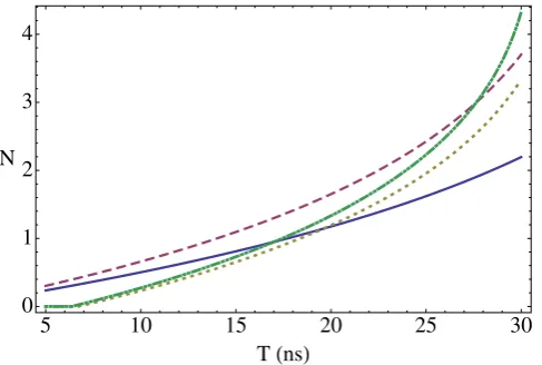
The state (55) is a multipartite entangled state. Entanglement can be extended to form a larger regular structure by means of the techniques described in this work. Within the approximations commented in, the section “Discrete and continuous motion” higher order entanglement resonances are completely suppressed. The time of the oscil-lation can be suitably chosen in order to generate a similar amount of entanglement between all the links (see Fig. 4). In particular, the reduced state of modes k=2 and k′ =5 after the first drive is given by
(
)
(
)
σ
σ
σ =
+ ( ) −
− + ( )
,
( ) ∼
( )
× ( )
( ) ( )
×
B B
B B
1 2
2 1
56
z z
25
251 2 2 2 251
251 251 2 2 2
For small h the state of the system remains pure to first order corresponding to a two-mode squeezed state with squeezing parameter r =B( )
25 251. However, when repeating the trajectory a large number of times to generate a
resonance, second order terms in the expansion of the Bogoliubov coefficients need to be included. These second order terms give rise to thermal noise quantified by (B25( )1 2) which in this case is given by Eq. (23). A similar
expres-sion holds for modes k=3 and k′ =4 after the first drive. The entanglement in state (56) can be quantified with the logarithmic negativity which yields in this case:
=
(
)
, − − + ( ) , ( ) ( ) ( ) B Bmax 0 log 1 2 57
25 251 251 2
and similarly for 34. Now we can drive the system at ωd=2π×12 GHz in order to entangle modes k=2 and
′ =
k 3. However, the initial state is no longer the vacuum. After the first drive the reduced covariance matrix of modes k=2 and k′ =3 is
σ =
, ( ) × × C C 0 0 58
23 25 2 2 34 2 2
where C25= + (1 B25( )1 2) and C34= + (1 B34( )1 2). The second drive transforms the state into
( )
σ = , ( )
∼ A B
B A 59
34
where the matrices above have the expression
(
)
σ = ( + ) + ( ) = − ( + ) + ( − ) . ( ) ( ) × ( ) × A BC C B
B C C C C
1
2 [ z ] 60
25 34 231 2 2 2
231 25 34 25 34 2 2
Note that if the amount of squeezing and entanglement generated with the first drive were exactly the same, i.e. C25=C34=C, then the state would be
(
)
(
)
σ σ σ = + ( ) − − + ( ) . ( ) ∼ ( ) × ( ) ( ) ( ) ×C B B
B B
2 1 2
2 1
61
z z
23
231 2 2 2 231
231 231 2 2 2
The fact that C25≠C34 adds a source of imperfection. The logarithmic negativity of the state in Eq. (59) is
(
)
(
)
= , ( + )( + ( ) ) − ( + ) + ( ) − + ( ) . ( ) ( ) ( ) ( )C C B
C C B C C B
max 0 ln 2
1
1 10 2 1 2
62
23
25 34 231 2
252 342 231 2 25 34 231 2 1 2
Two drives suffice to build up a linear graph. A third drive at ωd=20 GHz would entangle modes k=4 and
=
k 5, closing the square. In this case, the entanglement would be given by a similar expression as in Eq. (62), replacing B( )
231 by B45( )1. Figure 4 shows that a significant amount of entanglement is generated among the selected
[image:12.595.156.400.44.208.2]pairs of modes. The time of the drives can be chosen in such a way that all the pairs share a similar degree of entanglement. With all the above we have generated a H-graph state with square structure. Now, if we consider a rotation of the pump by an angle θ in one of the drives, say the last one, the corresponding correlation operators
Figure 4. Logarithmic negativity vs. time of the oscillatory motion for modes k= 2 and k′=5 (solid, blue),
=
are transformed to e−2iθa a
4 5, e a a2iθ 4 5† †. Thus, for θ= /π 2, the corresponding two-mode squeezing operator acquires
a minus sign. The effect is completely equivalent to replace B( )
451 by −B45( )1. Therefore, the effective Hamiltonian
acquires the form of the adjacency matrix of a square cluster state16. A square cluster state is a universal resource
for measurement-based quantum computation, provided that homodyne detection and photon-counting are possible. Both techniques are within reach of current circuit QED technology35,36.
Discussion
We have shown that it is possible to generate continuous-variable cluster states on electromagnetic cavity modes by choosing a suitable relativistic motion of the cavity. The entanglement grows linearly in time. The size of the lattice is determined by the choice of initial driving frequency, the amount of entanglement required between every mode and the desired length-to-height ratio of the square cluster. As a first experimental implementation, we propose a simple example of a four-mode square cluster state in a superconducting resonator with tuneable boundary con-ditions. This scheme is within reach of current circuit QED technology and would be the first demonstration of a multipartite continuous variable cluster state in cQED. An interesting avenue of research would be the extension to regimes of high squeezing levels, such as the ones required for fault-tolerant quantum computing with CV cluster states37. In brief, our main contribution is to implement cluster states in relativistic quantum field theory, paving
the way to relativistic quantum computing schemes. This is a step beyond the various proposed nonrelativistic implementations of continuous variable cluster states.
References
1. Ladd, T. D. et al. Quantum Computers. Nature 464, 45 (2010).
2. Alsing, P. M. & Fuentes, I. Observer dependent entanglement. Class. Quant. Grav 29, 224001 (2012).
3. Bruschi, D. E., Dragan, A., Lee, A. R., Fuentes, I. & Louko, J. Relativistic Motion Generates Quantum Gates and Entanglement Resonances. Phys. Rev. Lett. 111, 090504 (2013).
4. Bruschi, D. E., Louko, J., Faccio, D. & Fuentes, I. Mode-mixing quantum gates and entanglement without particle creation in periodically accelerated cavities. New Journal of Physics 15, 073052 (2013).
5. Moore, G. T. Quantum Theory of the Electromagnetic Field in a Variable- Length One-Dimensional Cavity. J. Math. Phys 11, 269 (1970).
6. Wilson, C. M. et al. Observation of the dynamical Casimir effect in a superconducting circuit. Nature 479, 376 (2011).
7. Zakka-Bajjani, E. et al. Quantum superposition of a single microwave photon in two different colour states. Nature Physics 7, 599 (2011).
8. Flurin, E., Roch, N., Mallet, F., Devoret, M. H. & Huard B. Generating Entangled Microwave Radiation Over Two Transmission Lines. Phys. Rev. Lett. 109, 183901 (2012).
9. Friis, N. et al. Relativistic Quantum Teleportation with Superconducting Circuits. Phys. Rev. Lett. 110, 113602 (2013). 10. Felicetti, S. et al. Dynamical Casimir Effect entangles artificial atoms. Phys. Rev. Lett. 113, 093602 (2014).
11. Felicetti, S. et al. Relativistic motion with superconducting qubits. Phys. Rev. B 92, 064501 (2015). 12. Weedbrook, C. et al. Gaussian quantmu information. Reviews of Modern Physics 84, 621 (2012).
13. Zhang, J. & Braunstein, S. L. Continuous-variable Gaussian analog of cluster states. Phys. Rev. A 73, 032318 (2006).
14. Menicucci, N. C et al. Universal Quantum Computation with Continuous-Variable Cluster States. Phys. Rev. Lett. 97, 110501 (2006). 15. Gu, M., Weedbrook, C., Menicucci, N. C., Ralph, T. C. & van Loock, P. Quantum computing with continuous-variable clusters. Phys.
Rev. A 79, 062318 (2009).
16. Menicucci, N. C., Flammia, S. T., Zaidi, H. & Pfister O. Ultracompact generation of continuous-variable cluster states. Phys. Rev. A 76, 010302 (2007).
17. Gottesman D., Kitaev A. & Preskill, A. Encoding a qubit in an oscillator. Phys. Rev. A 64, 012310 (2001).
18. Menicucci, N. C., Flammia, S. T. & Pfizer, O. One-Way Quantum Computing in the Optical Frequency Comb. Physical Review Letters 101, 130501 (2008).
19. Pysher, M., Miwa, Y., Shahrokhshahi, R., Bloomer, R. & Pfister, O. Parallel Generation of Quadripartite Cluster Entanglement in the Optical Frequency Comb. Phys. Rev. Lett. 107, 030505 (2011).
20. Friis, L., Lee, A. R. & Louko, J. Scalar, spinor and photon fields under relativistic cavity motion. Phys. Rev. D 88, 064028 (2013). 21. Birrell, N. D. & Davies, P. C. W. Quantum fields in curved space (Cambridge: University Press, 1982).
22. Bruschi, D. E., Fuentes, I. & Louko, J. Voyage to Alpha Centauri: Entanglement degradation of cavity modes due to motion. Phys. Rev. D 85, 061701 (2012).
23. Friis, N. & Fuentes, I. Entanglement generation in relativistic quantum fields. Journal of Modern Optics 60, 22 (2013).
24. Friis, N., Huber, M., Fuentes, I. & Bruschi, D. E. Quantum gates and multipartite entanglement resonances realized by nonuniform cavity motion. Phys. Rev. D 86, 105003 (2012).
25. Ji, J.-Y., Jung, H.-H., Park, J.-W. & Soh, K.-S. Production of photons by the parametric resonance in the dynamical Casimir effect. Phys. Rev. A 56, 4440 (1997).
26. Raussendorf, R. & Briegel, H. J. A One-Way Quantum Computer. Phys. Rev. Lett. 86, 5188 (2001). 27. Gottesman, D. Stabilizer Codes and Quantum Error Correction, Ph.D. thesis, Caltech (1997).
28. Kok, P. & Lovett, B. W. Introduction to Optical Quantum Information Processing (Cambridge University Press, 2010). 29. Braunstein, S. L. Squeezing as an irreducible resource. Phys. Rev. A 71, 055801 (2005).
30. Menicucci, N. C., Flammia, S. T. & van Loock, O. Graphical calculus for Gaussian pure states. Phys. Rev. A 83, 042335 (2011). 31. Alexander, R. N., Gabay, N. C. & Menicucci, N. C. Comment on “Towards universal quantum computation through relativistic
motion” arXiv:1312.6188 (2013).
32. Wallquist, M., Shumeiko, V. S. & Wendin, G. Selective coupling of superconducting charge qubits mediated by a tunable stripline cavity. Phys. Rev. B 74, 224506 (2006).
33. Sandberg, M. et al. Tuning the field in a microwave resonator faster than the photon lifetime. Appl. Phys. Lett. 92, 203501 (2008). 34. Wilson, C. M. et al. Photon generation in an electromagnetic cavity with a time-dependent boundary. Phys. Rev. Lett 105, 233907
(2010).
35. Chen, Y. F. et al. Microwave Photon Counter Based on Josephson Junctions. Phys. Rev. Lett 107, 217401 (2011).
36. Eichler, C. et al. Experimental State Tomography of Itinerant Single Microwave Photons. Phys. Rev. Lett 106, 220503 (2011). 37. Menicucci, N.C. Fault-Tolerant Measurement-Based Quantum Computing with Continuous-Variable Cluster States. Phys. Rev. Lett
Acknowledgements
The authors want to acknowledge G. Adesso, N. Friis and A. Lee for useful discussions. D.E.B. was in part supported by the UK Engineering and Physical Science Research Council grant number EP/J005762/1. I.F. and C.S acknowledge support from EPSRC (CAF Grant No. EP/G00496X/2 to I.F.). G.J. and P.D. would like to acknowledge funding from the Swedish Research Council and from the EU through the ERC and the projects PROMISCE and SQALEQIT. Financial support by Fundación General CSIC (Programa ComFuturo) is acknowledged by C.S.
Author Contributions
D.E.B. and I.F. conceived the project. D.E.B. and C.S. performed the computations. G.J. and P.K. provided theoretical assistance. P.D. revised the feasibility of the experimental proposal. I.F. supervised the project. All the authors contributed to the preparation of the manuscript.
Additional Information
Competing financial interests: The authors declare no competing financial interests.
How to cite this article: Bruschi, D. E. et al. Towards universal quantum computation through relativistic motion. Sci. Rep.6, 18349; doi: 10.1038/srep18349 (2016).