White Rose Research Online URL for this paper: http://eprints.whiterose.ac.uk/91047/
Version: Accepted Version
Article:
Leahy, C, Batley, R orcid.org/0000-0002-2487-850X and Chen, H (2016) Toward an
Automated Methodology for the Valuation of Reliability. Journal of Intelligent Transportation Systems: Technology, Planning, and Operations, 20 (4). pp. 334-344. ISSN 1547-2450 https://doi.org/10.1080/15472450.2015.1091736
(c) 2015, Taylor & Francis. This is an Accepted Manuscript of an article published by Taylor & Francis in Journal of Intelligent Transportation Systems: Technology, Planning, and Operations on 18/09/15 available online:
http://wwww.tandfonline.com/10.1080/15472450.2015.1091736
[email protected] https://eprints.whiterose.ac.uk/
Reuse
Unless indicated otherwise, fulltext items are protected by copyright with all rights reserved. The copyright exception in section 29 of the Copyright, Designs and Patents Act 1988 allows the making of a single copy solely for the purpose of non-commercial research or private study within the limits of fair dealing. The publisher or other rights-holder may allow further reproduction and re-use of this version - refer to the White Rose Research Online record for this item. Where records identify the publisher as the copyright holder, users can verify any specific terms of use on the publisher’s website.
Takedown
If you consider content in White Rose Research Online to be in breach of UK law, please notify us by
Towa r ds a n Automa ted Methodology for the Va lua tion of Relia bility
Author Information
Mr Christopher Leahy (Corresponding Author)
Email: [email protected]
Affiliation 1:
University of Leeds, Institute for Transport Studies, University Road, Leeds, LS2 9JT United
Kingdom
---
Dr Richard Batley
Email: [email protected]
Affiliation 1:
University of Leeds, Leeds, United Kingdom
---
Dr Haibo Chen
Email: [email protected]
Affiliation 1:
University of Leeds, Leeds, United Kingdom
Abstract
There is a significant body of research related to the valuation of reliability in transportation.
Such work has tended to rely on the Stated Preference (SP) methodology where respondents are
asked to make trade-offs between the mean and standard deviation of travel time. The literature
has suggested that a Revealed Preference (RP) methodology may provide an alternative means of
estimating a value of reliability. In this paper we show how emerging data sources reveal
travellers‟ preferences and, in combination with traditional choice modelling methods, can be
used to estimate a value of reliability. We illustrate this RP methodology using smart card data
from the multi-modal public transport network of London, UK. We are able to estimate a useable
„Reliability Ratio‟ for three of four public transport modes modelled, and account for an
unexpected result based upon the data available.
1.0 Introduction
There has been debate in the literature surrounding reliability in transportation and its formal
definition. Many authors use the term “travel time variation” (TTV) to indicate that some
measure of the width of the travel time distribution is actually what is being discussed. Although
research has introduced alternative methods for understanding reliability (e.g. the scheduling
approach of Small, 1982) it is this simple idea of the width of the travel time distribution that
will focus the discussion that follows.
It is clear from previous research that TTV is an important factor for explaining agents‟ travel
behaviour (Eddington, 2006), but its valuation remains an active research strand. It has been
noted that a Revealed Preference (RP) methodology may be instructive in the valuation of TTV,
but the situations where it can be effectively applied are rare (Bates et al, 2001), and
consequently this area remains underdeveloped. Instead there has been a reliance on Stated
Preference (SP) studies in order to value TTV (Ettema and Timmermans, 2006; Batley and
Ib ñez, 2012; Börjesson et al, 2012). Meta-analysis of these SP studies (e.g. Li et al, 2010;
Carrion and Levinson, 2012), as well as expert workshops (e.g. de Jong et al, 2009), have been
only partially successful in clarifying the value of TTV. What we will demonstrate in the work
that follows is that an RP approach, drawing upon existing discrete choice modelling methods,
can be employed to elicit a valuation of TTV.
This development is made possible by datasets generated by computerised systems associated
with the provision of transport services, where both aggregate route performance and traveller
behaviour are observed. Examples of such datasets include those collected from consumer
satellite navigation units, automatic number plate recognition cameras, and public transport
smart card usage. It is the latter that we will exploit to demonstrate application of our
methodology.
Moreover, the specific contributions of our paper are as follows:
1. To develop a RP methodology for the valuation of TTV
2. To utilise automatically generated datasets to provide valuation evidence for TTV
3. To demonstrate the use of such a dataset with existing discrete choice modelling
techniques
The paper is arranged as follows. In section two we will explore the concept of TTV and its
valuation, before examining the literature on valuing reliability using both RP and SP methods.
In section three we set up a basic TTV model and outline the discrete choice model
specifications relevant to the valuation of TTV. In section four we introduce an empirical dataset,
outline the context of the research in relation to the smart card literature, and apply the data with
choice modelling methods. In section five we discuss the modelling results and conclude by
commenting on the methodology developed.
2.0 Background
2.1 Travel Time Variation (TTV)
Travel time variation in the context we use it here refers to the widely known phenomenon that
undertaking a given trip will not always take the same amount of time. The exact nature of this
aspect of travel is considered in detail in the literature, which often differentiates between
recurrent variation and incident related delay (Bates et al, 2001). For the purposes of this paper
we take a simple approach; we assume that every available travel option is associated with a
Normal distribution of travel times, and furthermore can be accurately estimated and utilised in
travellers‟ decision making processes. This approach therefore explicitly draws a relationship
between the supply (or performance) of a transport system and the demand response from
travellers; an idea which is formalised by the mean-variance approach. This was initially
developed in the field of finance (Markowitz, 1959), but has become the most common
framework for understanding TTV.
The prevalence of the mean-variance approach is partly due to the simplicity of modelling the
marginal value of travel time alongside the marginal value of travel time variation. Adoption of
this approach has resulted in the acceptance of the Reliability Ratio (RR) in value of reliability
studies, which is given by the ratio of the marginal utility of time risk to the marginal utility of
mean travel time:
(1)
Where is the marginal utility of the mean travel time with respect to utility U, commonly
expected to be negative; and is the marginal utility of the standard deviation of travel time
with respect to U, also expected to be negative. The value of RR is therefore usually expressed as
a positive value. It is a value for RR that is estimated by the RP methodology outlined in the
remainder of the present paper.
2.2 The Stated Preference (SP) Approach to the Valuation of Travel Time
Variation
The preferred method of estimating the reliability ratio to date has been via SP surveys where
participants respond to a range of hypothetical travel options and are asked to make trade-offs
between travel time, TTV and cost.
A key reason for the prevalence of SP studies in this research area is that, while RP studies are
preferable in principle, practical situations where RP can be conducted successfully are rare
(Bates et al, 2001). The research community has therefore been largely comfortable in accepting
the SP method for valuing TTV, as evidenced by the number of studies performed (see the
review papers of Li et al, 2010; Carrion and Levinson 2012). SP route choice experiments have
yielded useful insights into the behaviour of travellers in relation to TTV; here we provide a brief
overview of recent studies, as a basis for developing an alternative method for estimating the
reliability ratio.
The SP study conducted in the much cited paper of Bates et al (2001) formed only part of the
contribution of that paper to the wider TTV literature. However section 6 of that paper, focussed
on the SP experiment warrants attention in its own right. Presentational issues related to prior
studies were considered in some depth; a debate which has become very much more prescient in
the TTV literature due to the complexity of the subject (for a later overview of the issues see
Tseng et al, 2008). It also employed a discrete choice experiment for the estimation of the value
of reliability. The study did not publish a RR due to confidentiality issues but nevertheless
confirmed TTV as highly valued by passengers.
The study of Hollander (2006) was focussed upon empirically estimating a RR using SP. This
work is quoted widely in the literature due to the outlying nature of its reported RR. Hollander
(2006) was an attempt to empirically compare the mean-variance approach to the alternative
scheduling approach (Small, 1982), which was performed using SP and discrete choice
modelling. This paper again considered the issue of survey presentation. Hollander‟s reported
reliability ratio of 0.1 was well below most other estimates. A possible explanation for the result
may be due to the survey being web-based, where respondent-researcher interaction was limited
and the demographic profile of respondents in the sample was unrepresentative of the wider
population.
What the aforementioned SP studies would seem to indicate is that a broad range of RR
estimates exist. Further evidence of this phenomenon is available in the meta-analyses of Li et al
(2010), Carrion and Levinson (2012) and Wardman and Batley (2014). The variation of RRs
might be due to a number of situational factors; for example the demographic characteristics of
respondents or mode availability. However the focus on presentational issues within the
literature (of Bates et al, 2001; Hollander 2009 among others) would suggest that they play an
important role in the estimation of accurate RRs, particularly given the complexity of the subject
(Tseng et al, 2008).
In addition to these problems, we might also draw the reader to well documented drawbacks of
hypothetical choice questionnaires, summarised in a recent review of travel time reliability
(Wardman and Batley, 2014). Wardman and Batley suggested that a strategic bias may be
observed given the contentiousness of TTV or lateness to travellers, particularly when the
purpose of the study is clear to the respondent. Furthermore we might add that the general
difficulties related to SP of misapprehension, fatigue and boredom experienced by respondents
might be exacerbated when dealing with the complexity of TTV issues.
Returning to the wide range of RR estimates found in the aforementioned meta-analyses, we now
focus on practical shortcomings of the use of SP studies to estimate a RR; these being the cost,
resource and knowledge required to conduct such studies. A possible alternative approach for
practitioners might be to ‟transfer‟ a pre-existing RR which was calculated under similar
circumstances (i.e. mode, geographic location etc.), but it is clear that an appropriate RR will not
be available for all situations. This does not take into account issues around context and
fungibility (Orr et al, 2012), yet this is the current position of practice (see WebTAG Unit A1.3
for evidence of this from the UK). The reason for this situation is a tacit acknowledgement of the
difficulty and resources required for conducting a unique choice experiment for each occasion
that a RR is required.
It is clear then from the above section that accurate estimates of RRs are necessary, but that
current methods to estimate it raise questions over their suitability. An alternative or
complementary solution to the estimation of RRs might be appropriate; one which overcomes:
how to make the appropriate choice of RR from the broad range of literature available
issues of SP respondent understanding of TTV
presentational issues specifically related to TTV SP surveys
general problems related to SP (strategic/protest responses)
cost/resource required to estimate a local RR
To address these issues we turn our attention to the less well research area of RP based estimates
of the RR.
2.3 The Revealed Preference (RP) Approach
A Revealed Preference (RP) approach in the transportation context is based upon what actual
traveller choices can tell us about their preferences – more specifically how they might trade-off
between travel time, TTV and other attributes of the journey. An RP based methodology would
overcome the issues highlighted in the previous section by incorporating participants‟ actual
decision making choices, including imperfections such as habitual behaviour and partial
information (Wardman and Batley, 2014). In overcoming the major deficiencies of SP we
therefore consider that RP is to be preferred (as suggested by Bates et al, 2001) and could
potentially elicit a more realistic RR. In addition we envisage an RP only approach would utilise
readily available datasets, the analysis of which could potentially be automated. This approach
could therefore provide a cost-effective, rapid, temporal/location specific method of estimating a
RR.
The general concerns with an RP-only approach are that insufficient situations might exist in a
dataset for effective estimation of parameters, as well as difficulty for the analyst in knowing the
completeness of travellers‟ information (as opposed to SP contexts where it can be considered
perfect). We also note the difficulty specific to mean-variance applications where travel time and
standard deviation of travel time have been found to be correlated (Batley et al, 2008; de Jong et
al, 2009). An additional criticism of RP based methods might be the restriction to situations
where appropriate data are available (Bates et al, 2001). However, as the present paper hopes to
demonstrate, this will become less of a problem as automatic data collection systems become
more prevalent.
The literature on RP based studies is limited, reflecting the difficulty of obtaining suitable and
sufficient datasets. The fullest account of their use in the TTV context is provided by Carrion and
Levinson (2012), from which we note the following key studies. Several RP studies have used
data from the SR-91 highway in California where drivers were observed making a choice
between a tolled express route and a standard un-tolled section of freeway. The most widely
cited of these studies (Small et al, 2005), analysed RP and SP data linked to census income data
(and other demographic data) using a mixed logit discrete choice model. Of interest is the
rejection of mean and standard deviation in their utility function, replaced with non-parametric
indicators. It is also of note that this model represented only a single mode (private car). The
combined RP/SP model gave an overall RR of 1.1, but an RP only model estimated separately
did not converge. Lam and Small (2001) was a closer attempt at an RP only methodology using
SR-91 data loop detector and demographic data, and estimated a RR of 0.77 for males and 1.45
for females. Other work has attempted to estimate reliability models based upon mode choice:
Bhat and Sardesai (2006) utilised an RP/SP methodology and incorporated public transport
modes into their model, estimating a RR of 0.26. Börjesson (2008) specified a mixed-logit
discrete choice model using RP and SP data and estimated an overall RR of 0.76; this paper
concluded that there are systematic differences between RP and SP datasets, in that RP
represents longer term adaptation by travellers to travel conditions.
Issues affecting these studies were the effort and resource required to estimate their models,
since they involved one or more of the following activities: contacting travellers directly to
obtain information about their route choices, matching SP records to observed number plates,
making assumptions about missing data, and/or staff involved in the study driving the route
repeatedly to estimate travel time distributions. None of the studies were able to observe both
supply and demand aspects of the transport systems of interest without directly asking
participants, and this need for interaction with travellers potentially introduced some of the
negative issues with SP that we outlined in the previous section. The mode choice modelled in
Börjesson (2008) was also reliant upon discrete departure times of the private car which may
have confused traveller preferences between car (which can usually depart continuously), and
bus which is subject to timetabled (discrete) departure times.
In the following section we address these issues by providing a methodology and framework for
the use of automatically collected data in estimating RRs without the need for extensive
surveying.
3.0 Modelling Framework
3.1 Choice and Risk
The phrase „choice under uncertainty‟ is often used in the literature on travel time variation,
however we do not use it here to avoid ambiguity. We instead use the phrase „choice under risk‟
to denote the situation where the distribution of outcomes is known by the traveller – a key
assumption as we progress with our methodology. Although perhaps unrealistic, this is a
simplifying assumption which will allow a RR to be estimated. Further work (and an extended
temporal dimension to the data) could take into account learning or knowledge effects on the part
of the traveller. We do comply with standard practice in the field in that we utilise the axioms of
expected utility theory (see von Neumann and Morgenstern, 1947). It has been shown that this
approach can provide results at odds with actual human behaviour (Kahnemann and Tversky,
1979), but nevertheless it is accepted in the transportation literature as a useful tool for
understanding risk. In accepting von Neumann and Morgenstern‟s (vNM) expected utility
framework, and implementing this through a discrete choice model, we assume that each of the
travellers observed will have well defined (complete) and stochastically transitive preferences.
3.2 Mean-Variance
The mean-variance framework of travel time variation will be utilised as a means for modelling
passengers‟ behavioural choices. The expected utility function of this framework takes the
following general form:
(2)
Where is equal to mean travel time and is the standard deviation of travel time, and and
are preference parameters for these variables. This representation of travel time risk has
received criticism for being dependent on a Normal distribution of travel times which is rarely
observed in reality (van Lint et al, 2008). Small et al (2005) recognised this issue and replaced
the mean travel time with the median, and the standard deviation with the difference between the
90th percentile and the median. Both the standard mean-variance and this non-parametric variant
will be tested in the empirical work that follows.
3.3 Data Requirements
The RP estimation of a reliability ratio will be based upon travellers‟ choice responses to
observable supply side metrics of a transport system. A requirement of this method is a dataset
which can provide estimates of mean and standard deviation of travel time and records of
travellers‟ route choices. Such datasets are becoming more prevalent and can include car based
trips (e.g. using ANPR systems) or public transport modes – with the latter being more
straightforward to implement due to the fixed nature of routing.
The setting up of an experiment must consider situations where all possible routes between an
origin-destination pair can be observed, and suitable sample sizes are available on each route.
There must also be some means of knowing which route is taken – through intermediate
observation or some indication at the origin or destination point.
3.4 Choice Model Specification
We will employ a discrete choice model to represent the route choice of the traveller in this
context. In the empirical section that follows, we apply three well-known discrete choice model
specifications, namely multinomial logit (MNL), mixed multinomial logit (MMNL) and
cross-nested logit (CNL) (a useful background to these specifications is provided by Train, 2009). The
logit model is the simplest and most well known of these, where the probability of individual n
choosing alternative i from choice set J ( , where ) is given by:
(3)
Where the observed portion of utility for individual n and alternative j is linear in
parameters and is therefore given by the term (where is a vector of observed variables
for individual n and alternative j).
The basic logit specification requires the condition of independence from irrelevant alternatives
(IIA) which is often not satisfied in real-world applications due to correlation between
alternatives. This correlation can be represented by either a mixture or nested choice model
specification. Our use of a mixture specification is with the purpose of representing
heterogeneity across travellers, in line with similar previous studies (Small et al, 2005; Bogers et
al, 2007). An alternative use of the mixed logit form is to induce correlation between the error
terms of similar alternatives, thereby representing a hierarchical or nested, structure; described as
the error components logit interpretation (Batley et al, 2004). The MMNL model is estimated
over a density of parameters, and therefore takes the general form:
(4)
In the case of the MMNL model, the value of is a weighted value of the MNL formula
estimated at different values of . The weighting of is given by the form of (Train,
2009).
A nested structure of the choice problem can be represented within the choice modelling
software by explicitly defining similar mode alternatives to be contained within a single nest.
More generally we note that an alternative might have membership of more than one nest,
meaning that a natural specification for the problem at hand is the cross-nested logit (CNL)
model specification. Here we provide the probability function for the Generalised Nested Logit
(GNL) model, which can be seen as generalised modelling framework wherein CNL represents a
special case. In particular, the restriction of dissimilarity parameter between modes in a single
nest k ( to be equal in equation 5 results in a CNL specification (Wen and Koppelman, 2001):
. (5)
The subscript k represents and indexation of the nests in the model: . denotes a
nest of alternatives. ik is the allocation parameter which signifies the proportion of membership
of alternative i to nest k.
4.0 Empirical Application of the Model
4.1 Smart Card Data
In our example we utilised a public transport smart card dataset. Public transport smart cards
provide a unique research opportunity in their own right (for an overview see Pelletier et al,
2011). Researchers have recognised the value of smart cards in observing travel behaviour (Choi
et al, 2012) and monitoring system performance (Jang, 2010), but we are unaware of any smart
card research which incorporates both supply and demand sides of a transport system.
The data available for this experiment were the trips made by a 5% sample of Oyster Card users
on the Transport for London (TfL) public transport network during a single, non-school holiday
month in 2011. The primary dataset contained details of each trip made, including an encrypted
user ID, mode, time, date and location of the beginning and ending for a trip on rail based modes.
Bus based trips did not have a recorded end point and so were excluded from the RP choice
modelling that follows. The impact of this is considered in the next section.
The initial dataset contained approximately 11 million Oyster transaction records. For the
purposes of this demonstration we decided to concentrate our analysis on the AM peak period.
To create the relevant dataset we removed non-AM peak journeys (beginning outside 07:00 –
10:00), weekend journeys, and all bus journeys. It was found that statistically significant
differences existed between the travel conditions during each of the three peak hours. Models
were therefore estimated over the AM peak as a whole and by each of the three peak hours.
Disaggregation of the data down to the hour level did however reduce the number of OD pairs
available.
4.2 Identification of Suitable Data
We were unable to utilise the full dataset for our modelling purposes as many trips were made
without indication of route choice. Consequently it was necessary to identify the origin
destination (OD) pairs where a mode choice was observable. This was done by creating an OD
trip matrix specific to each of the modes available. A database relationship was created between
each of these matrices to identify ODs where two or more modes were used with a count of
sample of travellers at 15 or greater. ODs were excluded where one of the choices was
dominated; i.e. where both the mean and standard deviation of travel time were lower for a given
option. Unfortunately two modes featured in the sample were represented on only three OD
pairs. Preliminary experiments showed that estimating parameters on such few choice situations
would lead to unreliable parameter estimates and therefore these two modes were removed.
These processes resulted in 31 candidate OD pairs being available for the AM peak model
estimation, giving a total of 4,140 usable records (an average of 134 trips per OD). A dataset of
the three individual peak hours (7-10) was also created, containing a subset of these 31 OD pairs
where the sample size was adequate in a single peak hour. Using this hour based dataset it would
be possible to estimate models where the travel conditions were related to the hour of travel (as
opposed to the whole AM peak period). This dataset consisted of 2,061 records.
The bus based smart card records did not include the time or location of a passenger alighting the
vehicle. This presented a challenge for accurately estimating both bus performance and
passenger behaviour. We therefore estimated choice model parameters based solely upon rail
based modes, and omitted the bus data from model estimation. An additional concern was that
there were no highway based modes in the study – including private car. We made the
simplifying assumption that car would (notionally) exist in an independent „non PT‟ nest, and
therefore the estimates within the PT nest were unbiased. The omission of the bus mode was
more problematic as this would likely cause bias within the PT nest.
To address this concern we created a list of all 62 origin and destination stations that were in the
choice dataset. Returning to the full dataset of 11 million records, we were able to identify all
travellers that interacted with these origins and destinations, including trips made using bus for
all or part of the trip. We were then able to link transfers between bus and other modes (drawing
upon the work of Seaborn et al, 2009), and thereby identify instances of travellers using bus for
all or part of their trip on one of the 31 OD pairs. Some evidence was found of a small number of
travellers using bus between five of the ODs, however the numbers were small (1 or 2 travellers
for each of these OD pairs). On reflection it was decided to proceed to the analysis stage with the
full complement of 31 AM peak OD pairs. An alternative would have been to exclude the OD
pairs where there was evidence of bus use, but much data would have been lost.
4.3 Data Analysis
To populate the mean-variance part of the choice model, we assigned an ID to each of the
traveller records within the dataset based upon which OD they were travelling between. We
assigned a further separate ID to each traveller based upon the mode of transport they utilised.
Within this dataset, the use of three public transport modes was identified:
Light Rail – also referred to as the Docklands Light Railway, or DLR
Metro – also referred to as London Underground, or LU
Heavy Rail – standard heavy rail services, including London Overground. Referred to as
„Rail‟ in the model specification
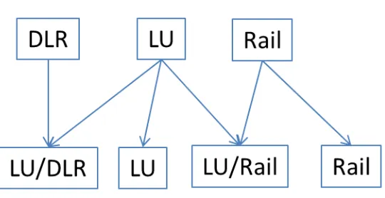
Some journeys consisted of two of these modes and so two further modes choices were created
which were a composite of two of the other modes. Figure 1 demonstrates how each of the six
modes was composed. The method of grouping suggested that there would be correlation
between the modes when they contained a common method of transport. This supports use of a
cross nested logit structure when modelling this data (multinomial logit and mixed multinomial
logit models will also be estimated, in line with many similar studies in this field (Carrion and
Levinson, 2012).
For any one OD pair, there were only two of the four modes available. We were able to calculate
a sample mean travel time and standard deviation by using both OD and mode ID (denoted by
subscript m) – i.e. each OD had two sets of mean-variance values; one for each of the public
transport travel choices available to the traveller. We present the results of this process in
Appendix 1 of the present paper. Each individual record, representing a single trip, has assigned
to it the mean and standard deviation for the two options available.
A concern remained regarding the issue raised in the literature of correlation between mean and
standard deviation of travel time (Batley et al, 2008; de Jong et al, 2009), however our analysis
based upon the information in Appendix 1 suggested that this was not an issue in the present
context.
5.0 Choice Modelling
The models in this section were estimated using Biogeme (Bierlaire, 2003). We utilised four
choice model specifications: multinomial logit, mixed logit, cross nested logit and cross nested
logit with mixture parameters. Preliminary work indicated significant differences between travel
time and risk parameter estimates for each mode: therefore interaction terms between the
mean-variance parameters and mode-based alternative specific constants (ASCs) are included where
possible. We present results from the four separate model specifications for the AM peak time
period. We also estimated these same model specifications with an alternative dataset where a
mean and standard deviation term were calculated for each of the three peak hours as described
in section 4.2. This process did not improve the results or model fit when compared to the overall
AM Peak models and are not included further in the paper. Another alternative approach is the
specification of a percentile based utility function as described in section 3.2. When modelled,
this specification did not offer an improved model fit or results. Therefore the results reported in
Table 1 are related to the standard mean-variance specification where travel time and standard
deviation are calculated for the entire peak period. The expected utility for individual n is
therefore determined by the mode used and the OD pair:
(6)
Where is the expected utility for individual n based on their OD pair (OD) and mode
choice (m). and represent the mean and standard deviation of the chosen OD pair
and mode combination. represents the marginal utility of mean travel time. Similarly,
represents the marginal utility of travel time variation. The error term, , varies between
individuals, denoted by subscript n.
When using a mixed model specification, the parameter estimates were specified to be Normally
distributed; this was judged appropriate to allow for a proportion (but not all) of the travellers to
exhibit behaviour that placed a positive marginal utility on travel time and risk. We utilised a
2-tailed t-test for significance of all parameter estimates.
5.1 AM Peak Model Estimates
The AM peak models were run using the non-dominated dataset containing 4,140 trip records.
Alternative-specific constants (ASCs) were estimated in all cases, except for Metro (London
Underground) fixed to zero as the reference case. We found that interaction terms between the
mode ASCs and mean and standard deviation improved the model results, and they were
therefore included in the MNL and MMNL models. The inclusion of interaction terms within the
CNL models caused issues, and they were not therefore retained. We report four key model
specifications here:
Model 1 was a basic MNL specification with three ASCs estimated for each of the modes
other than London Underground shown in Figure 1. and were estimated for the
marginal utilities of mean travel time and standard deviation respectively. Each of the
ASCs was interacted with mean travel time and standard deviation, so as to give mode
specific estimates of the first and second moments.
Model 2 utilised a CNL structure as indicated in Figure 1. The term defined in equation
5 was allowed to vary, and each hybrid mode could belong to two nests i.e. LU/DLR
could belong to both „LU‟ and „DLR‟ nests. In preliminary testing, the inclusion of
interaction terms caused issues with the ASCs and allocation parameters, and they were
therefore omitted from the final model. The ASCs and s were specified in the same
manner as Model 1.
Model 3 was a mixed MNL model, specified identically to Model 1 with the exception
that the estimate on mean travel time and standard deviation was allowed to vary to
represent stochastic traveller preferences.
Model 4 was a combination of Models 2 and 3; it included the CNL structure and nesting
parameters of Model 2, and the mixture parameters for the marginal utilities of travel
time and risk from Model 3. Preliminary estimation of Model 4 showed a similar issue to
Model 2, in that the model would not converge when the ASCs and interaction terms
were specified. In common with Model 2, the interaction terms were therefore
omitted.With reference to Table 1, the parameter estimates of Model 1 are statistically
significant with the exception of the risk parameter for the heavy rail mode and the travel
time parameter for the LU/DLR mode. There are significant differences between the
modes all else equal, as indicated by the ASCs (defined in relation to London
Underground only mode). Furthermore, the significance of most of the mean-variance
interaction terms shows that passengers‟ attitudes towards travel time and risk vary across
modes. We observe that the marginal utility of travel time is negative as expected across
all modes. We also observe that the marginal utility of risk is negative on three of the four
modes modelled. The model fit indicated by the adjusted R2 (of 0.31) is acceptable.
The CNL specification in Model 2 results in only one parameter estimate for both travel time and
travel time risk. Both are negative which suggests a rejection of the null hypothesis, however the
t-statistic of 1.95 on the risk parameter means that strictly speaking the null cannot be rejected at
the 5% level. The ASCs are all significant, indicating differences between the modes all else
equal. The R2 and final log-likelihoodmeasures of model fit are lower than Model 1, indicating a
poorer fit to the data.
Model 3 estimates significant parameters similar to those estimated in Model 1, where the risk
parameter for Rail is found to be insignificantly different from the base case. The mixture
parameter on the marginal utility of travel time is significantly different from zero, but the
mixture parameter on travel time risk is not. The marginal utility of travel time is negative for all
four modes, and the risk parameter is negative on three of the four modes. The R2 and
log-likelihood measures indicate that the fit of Model 3 is an improvement over Models 1 and 2.
In Model 4 it is found that both travel time and travel time risk parameters are significant and
negative. All ASCs are significantly different from zero. In contrast to Model 3, both mixture
parameters are statistically significant at the 5% confidence level. The fit of this model to the
data is however the poorest of the four models estimated.
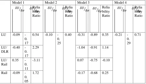
Table 2 shows the reliability ratios (RRs) estimated. Single RRs were estimated from Models 2
and 4 as they did not contain interaction terms for each mode. Travel time and travel time risk
are generally assumed to be viewed as a „bad‟ by travellers. Therefore, negative parameter
estimates for mean travel time and standard deviation are expected, resulting in a positively
valued RR. We apply these criteria here and consider negative RRs and RRs calculated using
positive marginal utilities of travel time and risk to be of less practical use.
Focussing on Models 1 and 3, valid RR values have been calculated for three of the four modes
included in this study. These modes are LU, LU/DLR and Rail. The positive parameter estimate
of risk on the LU/Rail mode meant that a negative (and unsatisfactory) RR was estimated for this
mode. We use meta-analysis of Carrion and Levinson (2012) as a comparator for our results.
They reported average RRs from 17 studies, with a range of 0.1 to 2.51 and a mean average of
1.09. The RR estimates for the LU mode are 0.54 and 0.35, which are low compared to the
comparator value of 1.09, but are not unreasonable in relation to some estimates in the literature
(e.g. Bhat and Sardesai, 2006). Estimates for the LU/DLR RR of 2.29 and 1.14 are reasonable in
light of the comparison value. The estimates for the mode LU/Rail were negative across all four
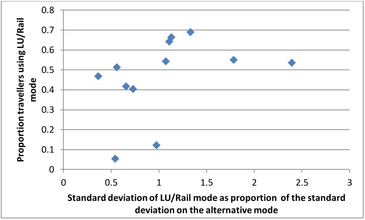
models, as the parameter estimate of risk for this mode was always estimated as positive. Further
investigation into this counter-intuitive result reveals that when the LU/Rail mode is available,
travellers are more likely to use it when the standard deviation is higher on this mode when
compared to the alternative. This is plotted for all twelve LU/Rail OD pairs, where a general
positive relationship between the variables is indicative of risk seeking behaviour. It should be
noted that these same travellers are also strongly averse to travel time.
Mode specific parameter estimates were not made by Models 2 and 4. This results in only one
RR value estimated from each as shown in Table 2. Whilst acknowledging that the risk
parameter in Model 2 is borderline significant (as shown in Table 1), the RR implied by this
model was 0.40. Although low, this is acceptable in relation to the literature. The RR of 0.71
implied by Model 4 appears more in line with the literature, and demonstrates a degree of
sensitivity of the RR to the model specification.
These model results provide evidence that a dataset such as that provided by a public transport
smart card system can be used in the estimation of marginal utilities of travel time and travel
time risk. Model 1 provides acceptable RR estimates for three of the four modes modelled, in the
range 0.54 to 2.29. Model 3 also estimates three useable RR values between 0.25 and 1.14.
Models 2 and 4, without interaction terms, estimated single RR values which could be used over
all modes in an appraisal.
6.0 Conclusion
In this paper we have demonstrated a method of estimating a reliability ratio using revealed
preference data. We initially outlined the benefit of undertaking the research; both in terms of the
limitations of the alternative stated preference method (general suitability, high survey cost) and
the positive aspects of revealed preference (realism, low survey cost). We combined standard
economic and choice modelling approaches to form the basis for introducing the possibility of
estimating the reliability ratio from automatically collected data only. We then used one such
data source, public transport smart card data, to demonstrate the method. We were able to
estimate a realistic RR across three alternative modes during the AM peak period. The majority
of these estimates were within an acceptable range when compared to the literature. A range of
RR estimates in the literature highlights the importance of estimating a RR which is relevant to
its application, an issue which the methodology outlined in this paper could provide a solution.
The unexpected result of a positive risk parameter on one of the modes was partially accounted
for by the data; travellers were seemingly primarily motivated by travel time savings and not by
travel time risk. In addition, a greater sample size and therefore an increased number of OD pairs
in the choice dataset may assist with this issue. There is also the possibility that there are omitted
variables from our model which bias the results. For example, station size or accessibility to
platforms may impact upon travellers mode choice, but this was not explicitly represented in the
model. The relatively small sample sizes at the OD level of aggregation meant that it was mainly
large stations that featured within the dataset, and a station size variable could not be easily
modelled. Such omitted variables are likely to be the reason for seemingly dominated choice
options which were nevertheless utilised by travellers.
The assumption of perfect knowledge on the part of every passenger is also unrealistic. A
development of the RP method would take into account variability in experience of passengers
on a route – this could be performed more accurately where the dataset covered a longer
temporal duration than one month. In addition, future research might consider datasets that
contain a cost variable so that monetary values of reliability can be estimated directly, thus
overcoming the issue of fungibility when utilising a RR alongside separately estimated values of
time (Orr et al, 2012).
We would recommend that further empirical research is conducted, where full population smart
card datasets are collected to overcome issues with sample sizes and to include a wider range of
modes and geographic locations. Additional data collection to take account of further variables
should also improve the robustness of RP choice models.
Acknowledgements
The authors would like to thank both the ESRC White Rose Doctoral Training Centre and
Transport for London for funding this research. We would also like to thank the reviewers for
their comments on earlier versions of the paper. The work contained within this paper is the sole
responsibility of the authors and does not reflect the views of the funding organisations or
reviewers.
References
BATES, J., POLAK, J., JONES, P. & COOK, A. (2001). The valuation of reliability for personal
travel. Transportation Research Part E: Logistics and Transportation Review, 37, 191-229.
BATLEY, R. P., TONER, J. P., & KNIGHT, M. J. (2004). A mixed logit model of UK
household demand for alternative-fuel vehicles. Rivista Internazionale Di Economia Dei
Trasporti. 31, 55-77.
BATLEY, R., GRANT-MULLER, S., NELLTHORP, J., DE JONG, G., WATLING, D.,
BATES, J., HESS, S. & POLAK, J. (2008). Multimodal Travel Time Variability. Institute for
Transport Studies. Leeds, UK.
BATLEY, R. & IBÁÑEZ, J. N. (2012). Randomness in preference orderings, outcomes and
attribute tastes: An application to journey time risk. Journal of Choice Modelling, 5, 157-175.
BIERLAIRE, M. (2003). BIOGEME: A free package for the estimation of discrete choice
models , Proceedings of the 3rd Swiss Transportation Research Conference, Ascona,
Switzerland.
BHAT, C. R. & SARDESAI, R. (2006). The impact of stop-making and travel time reliability on
commute mode choice. Transportation Research Part B: Methodological, 40, 709-730.
BOGERS, E., VITI, F., HOOGENDOORN, S. & VAN ZUYLEN, H. (2007). Valuation of
Different Types of Travel Time Reliability in Route Choice: Large-Scale Laboratory
Experiment. Transportation Research Record: Journal of the Transportation Research Board,
1985, 162-170.
BÖRJESSON, M. (2008). Joint RP-SP data in a mixed logit analysis of trip timing decisions.
Transportation Research Part E: Logistics and Transportation Review, 44 (6), 1025–1038.
BÖRJESSON, M., ELIASSON, J. & FRANKLIN, J. P. (2012). Valuations of travel time
variability in scheduling versus mean–variance models. Transportation Research Part B:
Methodological, 46, 855-873.
CARRION, C. & LEVINSON, D. (2012). Value of travel time reliability: A review of current
evidence. Transportation Research Part A: Policy and Practice, 46, 720-741.
CHOI, J., LEE, Y., KIM, T. & SOHN, K. (2012). An analysis of Metro ridership at the
station-to-station level in Seoul. Transportation, 39, 705-722.
DEPARTMENT FOR TRANSPORT, (2014). WebTAG Unit A1.3: User and Provider Impacts.
London
ETTEMA, D. & TIMMERMANS, H. (2006). Costs of travel time uncertainty and benefits of
travel time information: Conceptual model and numerical examples. Transportation Research
Part C: Emerging Technologies, 14, 335-350.
HOLLANDER, Y. (2006). Direct versus indirect models for the effects of unreliability.
Transportation Research Part A: Policy and Practice, 40, 699-711.
HOLLANDER, Y. (2009). What do we really know about travellers‟ response to unreliability?
The International Choice Modelling Conference, Harrogate, UK
JANG, W. (2010). Travel Time and Transfer Analysis Using Transit Smart Card Data.
Transportation Research Record: Journal of the Transportation Research Board, 2144, 142-149.
DE JONG, G., KOUWENHOVEN, M., KROES, E., RIETVELD, P. & WARFFEMIUS, P.
(2009). Preliminary Monetary Values for the Reliability of Travel Times in Freight Transport.
European Journal of Transport and Infrastructure Research, 9, 83-99.
EDDINGTON, R. (2006). The Eddington Transport Study. HM Treasury. London, UK.
KAHNEMANN, D. & TVERSKY, A. (1979). Prospect theory: An analysis of decision under
risk. Econometrica: Journal of the Econometric Society, 263-291.
KNIGHT, F. H. (1921). Risk, Uncertainty, and Profit. Hart, Schaffner, and Marx Prize Essays,
no. 31. Boston and New York: Houghton Mifflin.
LAM, T. C. & SMALL, K. A. (2001). The value of time and reliability: measurement from a
value pricing experiment. Transportation Research Part E: Logistics and Transportation
Review, 37, 231-251.
LI, Z., HENSHER, D. A. & ROSE, J. M. (2010). Willingness to pay for travel time reliability in
passenger transport: A review and some new empirical evidence. Transportation Research Part
E: Logistics and Transportation Review, 46, 384-403.
VAN LINT, J. W. C., VAN ZUYLEN, H. J. & TU, H. (2008). Travel time unreliability on
freeways: Why measures based on variance tell only half the story. Transportation Research
Part A: Policy and Practice, 42, 258-277.
ORR, S. HESS, S & SHELDON, R (2012) Consistency and fungibility of monetary valuations in
transport: an empirical analysis of framing and mental accounting effects. Transportation
Research Part A: Policy and Practice, 46 (10). 1507 - 1516.
PELLETIER, M.-P., TRÉPANIER, M. & MORENCY, C. (2011). Smart card data use in public
transit: A literature review. Transportation Research Part C: Emerging Technologies, 19,
557-568.
SEABORN, C., ATTANUCCI, J. & WILSON, N. (2009). Analyzing Multimodal Public
Transport Journeys in London with Smart Card Fare Payment Data. Transportation Research
Record: Journal of the Transportation Research Board, 2121, 55-62.
SMALL, K. A. (1982). The Scheduling of Consumer Activities: Work Trips. The American
Economic Review, 72, 467-479.
SMALL, K. A., WINSTON, C. & YAN, J. (2005). Uncovering the Distribution of Motorists'
Preferences for Travel Time and Reliability. Econometrica, 73, 1367-1382.
TRAIN, K. E., (2009). Discrete choice methods with simulation. 2nd Edition, Cambridge
University Press.
TSENG, Y.-Y., VERHOEF, E., DE JONG, G., KPOUWENHOVEN, M. & VAN DER HOORN,
T. (2008). A pilot study into the perception of unreliability of travel times using in-depth
interviews. Journal of Choice Modelling, 2, 8-28.
WARDMAN, M. & BATLEY, R. (2014). Travel time reliability: a review of late time
valuations, elasticities and demand impacts in the passenger rail market in Great Britain.
Transportation, 1-29.
WEN, C.-H. & KOPPELMAN, F. S. (2001). The generalized nested logit model. Transportation
Research Part B: Methodological, 35, 627-641.
Appendix 1 – Observed traveller choices and mean-variance performance data for the AM peak
OD pairs
Mode 1 Mode 2
Mod e 1 Mode 2 Cou nt Me an Medi an St Dev Cou nt Me an Medi an St Dev Arnos Grove_Canary
Wharf LU
LU/D
LR
62.0
0
55.
48 57.00 13.1
9
20.0
0
55.
55 55.00 7.04
Woodside Park_Canary
Wharf LU
LU/D
LR
52.0
0
55.
44 55.00 5.07 40.0
0
56.
00 55.50 3.65
Morden_Canary Wharf LU
LU/D
LR
142.
00 50.
35 49.00 6.04 22.0
0
52.
91 52.00 4.16
East Finchley_Canary
Wharf LU
LU/D
LR
27.0
0
47.
22 47.00 6.31 24.0
0
49.
25 49.00 3.64
Debden_Canary Wharf LU
LU/D
LR
54.0
0
46.
35 45.00 5.19 26.0
0
46.
77 47.50 3.51
Colliers Wood_Canary
Wharf LU
LU/D
LR
69.0
0
44.
94 43.00 5.20 19.0
0
49.
21 48.00 4.30
Hornchurch_Canary
Wharf LU
LU/D
LR
85.0
0
44.
41 43.00 5.57 23.0
0
43.
00 42.00 7.05
Hampstead_Canary
Wharf LU
LU/D
LR
30.0
0
44.
17 43.00 4.96 39.0
0
44.
92 45.00 3.25
Kentish Town_Canary
Wharf LU
LU/D
LR
19.0
0
38.
95 39.00 3.76 32.0
0
37.
38 36.50 4.21
Barkingside_Canary
Wharf LU
LU/D
LR
37.0
0
38.
70 38.00 3.84 15.0
0
41.
67 42.00 1.95
Buckhurst Hill_Canary
Wharf LU
LU/D
LR
119.
00 38.
50 37.00 6.85 15.0
0
41.
67 41.00 6.24
Shepherds
Bush_Canary Wharf LU
LU/D
LR
96.0
0
37.
47 36.00 5.56 28.0
0
43.
25 42.00 3.30
Clapham South_Canary
Wharf LU
LU/D
LR
355.
00 36.
50 35.00 6.06 43.0
0
41.
65 40.00 5.79
Gants Hill_Canary
Wharf LU
LU/D
LR
143.
00 33.
21 32.00 5.44 34.0
0
37.
21 37.00 4.26
South
Woodford_Canary
Wharf LU
LU/D
LR
226.
00 31.
78 31.00 5.16 73.0
0
35.
08 34.00 4.37
Snaresbrook_Canary
Wharf LU
LU/D
LR
100.
00 31.
50 30.00 6.21 23.0
0
34.
35 33.00 5.84
Old Street_Canary
Wharf LU
LU/D
LR
71.0
0
23.
03 22.00 4.50 50.0
0
24.
58 24.00 3.60
Leyton_Canary Wharf LU LU/D LR 179. 00 22.
08 21.00 5.06 34.0
0
26.
21 26.00 4.05
Ealing
Broadway_Kings Cross LU
LU/R
ail
49.0
0
41.
67 41.00 8.17 35.0
0
42.
86 42.00 5.36
Paddington_Old Street LU
LU/R
ail
25.0
0
30.
68 33.00 13.9
3
22.0
0
35.
45 34.00 5.10
Walthamstow
Central_Farringdon LU
LU/R
ail
108.
00 32.
79 32.00 4.53 15.0
0
35.
40 36.00 4.42
Tooting
Broadway_Victoria LU
LU/R
ail
280.
00 27.
00 26.00 5.35 16.0
0
28.
75 28.50 2.91
Vauxhall_Canary
Wharf LU
LU/R
ail
37.0
0
31.
14 30.00 5.20 73.0
0
28.
67 27.00 5.89
Seven Sisters_Bethnal
Green LU
LU/R
ail
20.0
0
37.
15 36.50 2.30 23.0
0
26.
74 26.00 5.51
Harrow On The
Hill_Marylebone LU
LU/R
ail
19.0
0
33.
89 33.00 4.54 34.0
0
21.
21 19.50 5.04
Brixton_Victoria LU Rail
546.
00 13.
73 13.00 2.53 23.0
0
12.
13 10.00 4.73
Richmond_Victoria Rail
LU/R
ail
68.0
0
28.
91 28.00 6.28 46.0
0
39.
15 39.00 4.59
Motspur Park_Victoria Rail LU/R 19.0 33. 32.00 5.97 20.0 38. 37.50 3.35
ail 0 37 0 20
Wimbledon_London
Bridge Rail
LU/R
ail
16.0
0
38.
63 36.00 8.21 19.0
0
36.
47 34.00 8.83
Earlsfield_London
Bridge Rail
LU/R
ail
18.0
0
34.
61 35.00 3.22 22.0
0
31.
23 30.00 5.75
Clapham
Junction_London
Bridge Rail
LU/R
ail
50.0
0
29.
50 29.50 4.01 111.
00 26.
07 24.00 5.34
Abbreviations:
Mean – Sample mean travel time for OD and mode
St Dev - Sample standard deviation of travel time for OD and mode
LU – London Underground
DLR – Docklands Light Rail
Rail – Overground and/or National Rail
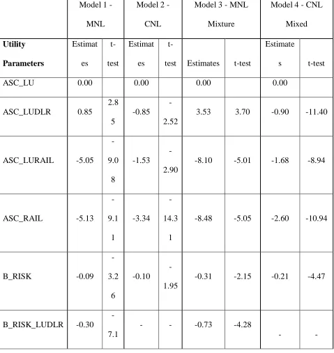
Table 1 – Parameter estimates and summary statistics of AM peak choice models
Model 1 -
MNL
Model 2 -
CNL
Model 3 - MNL
Mixture
Model 4 - CNL
Mixed Utility Parameters Estimat es t-test Estimat es
t-test Estimates t-test
Estimate
s t-test
ASC_LU 0.00 0.00 0.00 0.00
ASC_LUDLR 0.85
2.8
5
-0.85
-2.52
3.53 3.70 -0.90 -11.40
ASC_LURAIL -5.05
-9.0 8 -1.53 -2.90
-8.10 -5.01 -1.68 -8.94
ASC_RAIL -5.13
-9.1 1 -3.34 -14.3 1
-8.48 -5.05 -2.60 -10.94
B_RISK -0.09
-3.2 6 -0.10 -1.95
-0.31 -2.15 -0.21 -4.47
B_RISK_LUDLR -0.30
-7.1
- - -0.73 -4.28
- -
4
B_RISK_LURAI
L
0.44
5.7
8 - -
0.38 2.28
- -
B_RISK_RAIL 0.04
0.4
5 - -
0.14 0.68
- -
B_TIME -0.17
-9.1 3 -0.25 -2.87
-0.89 -3.61 -0.29 -4.21
B_TIME_LUDL
R
-0.01
-1.1
4 - -
-0.03 -2.26
- -
B_TIME_LURAI
L
0.06
3.5
0 - -
0.14 3.17
- -
B_TIME_RAIL 0.12
7.7
8 - -
0.21 4.46
- -
B_RISK_MIXTU
RE
- -
- -
-0.15 -0.45 -0.23 -2.01
B_TIME_MIXT
URE
- -
- -
1.12 3.48 0.32 2.65
Model
Parameters
DLR Nest - - 1.00 0.00 - - 1.00 0.00
- LUDLR 0.76 1.44 0.64 2.85
LU Nest - - 0.73 2.36 - - 1.00 0.01
- LUDLR 0.25 0.47 0.36 1.58
- LURAIL 0.86 1.63 0.95 18.18
Rail Nest - - 0.22 2.97 - - 8.18 0.52
- LURAIL 0.15 0.28 0.05 1.03
Summary
Statistics
n 4,140 4,140 4,140 4,140
Adjusted R2 0.312 0.289 0.318 0.281
Final
log-likelihood
-1964.70
-2028.26
-1944.63 -2049.98
Table 2 – Reliability ratios estimated by Models 1 to 4
Model 1 Model 2 Model 3 Model 4
Relia bility Ratio Relia bility Ratio Relia bility Ratio Relia bility Ratio
LU -0.09 -0. 17
0.54 -0.10 -0. 25
0.40 -0.31 -0.89 0.35 -0.21 -0. 29
0.71
LU/ DLR
-0.40 -0. 17
2.29 -1.04 -0.91 1.14
LU/ Rail
0.35 -0. 11
-3.11 0.07 -0.75 -0.10
Rail -0.09 -0. 05
1.72 -0.17 -0.68 0.25
Figure 1 – Mapping of rail based modes to composite modes used in subsequent modelling
Figure 2 – OD plot of the standard deviation of LU/Rail mode against proportion using the
LU/Rail mode
0 0.1 0.2 0.3 0.4 0.5 0.6 0.7 0.8
0 0.5 1 1.5 2 2.5 3
P
ro
p
o
rt
io
n
t
ra
v
e
ll
e
rs
u
si
n
g
L
U
/R
a
il
m
o
d
e
Standard deviation of LU/Rail mode as proportion of the standard deviation on the alternative mode