Testing models of ice cap extent, South Georgia, sub-Antarctic

(1)

This is a repository copy of Testing models of ice cap extent, South Georgia, sub-Antarctic.

White Rose Research Online URL for this paper:

http://eprints.whiterose.ac.uk/107105/

Version: Accepted Version

Article:

Barlow, NLM orcid.org/0000-0002-2713-2543, Bentley, MJ, Spada, G et al. (6 more

authors) (2016) Testing models of ice cap extent, South Georgia, sub-Antarctic.

Quaternary Science Reviews, 154. pp. 157-168. ISSN 0277-3791

https://doi.org/10.1016/j.quascirev.2016.11.007

© 2016, Elsevier. Licensed under the Creative Commons

Attribution-NonCommercial-NoDerivatives 4.0 International

http://creativecommons.org/licenses/by-nc-nd/4.0/

[email protected] https://eprints.whiterose.ac.uk/ Reuse

Unless indicated otherwise, fulltext items are protected by copyright with all rights reserved. The copyright exception in section 29 of the Copyright, Designs and Patents Act 1988 allows the making of a single copy solely for the purpose of non-commercial research or private study within the limits of fair dealing. The publisher or other rights-holder may allow further reproduction and re-use of this version - refer to the White Rose Research Online record for this item. Where records identify the publisher as the copyright holder, users can verify any specific terms of use on the publisher’s website.

Takedown

If you consider content in White Rose Research Online to be in breach of UK law, please notify us by

(2)

1

Testing models of ice cap extent, South Georgia, sub-Antarctic.

Barlow, N.L.M.1,2*_{, Bentley, M.J.}1_{, Spada, G.}3_{, Evans, D.J.A.}1_{, Hansom, J.D.}4_{, Brader, M.D.}1_{, White, D.A.}5_,

Zander, A.6_{, Berg, S.}7

1_{Department of Geography, Durham University, South Road, Durham, DH1 3LE, UK}

2_{School of Earth and Environment, University of Leeds, Leeds, LS2 9JT, UK}

3_{Dipartimento di Scienze Pure e Applicate (DiSPeA) Urbino University ''Carlo Bo'', Urbino, Italy}

4_{School of Geographical and Earth Sciences, University of Glasgow, Glasgow, G12 8QQ, UK}

5_{Institute for Applied Ecology, University of Canberra, Canberra, ACT 2617, Australia.}

6_{Institute of Geography, University of Cologne, Albertus-Magnus-Platz, 50923 Cologne, Germany}

7 _{Institute of Geology and Mineralogy, University of Cologne, Zülpicher Str. 49a, 50674 Cologne,}

Germany

* Corresponding author: [email protected] +44 113 343 3761

Keywords

(3)

2

Abstract

The extent of Last Glacial Maximum ice in South Georgia is contested, with two alternative

hypotheses: an extensive (maximum) model of ice reaching the edge of the continental shelf, or a

restricted (minimum) model with ice constrained within the inner fjords. We present a new relative

sea-level dataset for South Georgia, summarising published and new geomorphological evidence for

the marine limit and elevations of former sea levels on the island. Using a glacial isostatic adjustment

model (ALMA) specifically suited to regional modelling and working at high spatial resolutions,

combined with a series of simulated ice-load histories, we use the relative sea-level data to test

between the restricted and extensive ice extent scenarios. The model results suggest that there was

most likely an extensive Last Glacial Maximum glaciation of South Georgia, implying that the island

was covered by thick (>1000 m) ice, probably to the edge of the continental shelf, with deglaciation

occurring relatively early (ca. 15 ka BP, though independent data suggest this may have been as early

as 18 ka). The presence of an extensive ice cap extending to the shelf edge would imply that if there

were any biological refugia around South Georgia, they must have been relatively localised and

(4)

3

Rationale and background

Though limited in size, the extent of glaciations of the sub-Antarctic islands, such as South Georgia, is

of considerable interest due to their position in the Southern Ocean, providing a potential link

between the climates of South America and West Antarctica (Hall, 2009; Hodgson et al., 2014a;

2014b). Moreover, the extent of ice has important implications as to whether the sub-Antarctic

islands acted as glacial refugia for biota (Barnes et al., 2006; Barnes et al., 2016; Hodgson et al., 2014b;

Hogg et al., 2011; Thatje et al., 2008). Though the contribution of the potential ice mass on South

Georgia to global sea level will be modest, recent changes in glacier extent in response to 20th_century

warming (Cook et al., 2010; Gordon et al., 2008) demonstrates the sensitivity of maritime South

Georgia to changes in climate and oceanographic forcing by the Southern Ocean. During the global

Last Glacial Maximum (LGM), ice on South Georgia expanded (Bentley et al., 2007; Hodgson et al.,

2014b; Sugden and Clapperton, 1977) but there remains significant debate about the maximum ice

extent reached during this time. Two widely divergent models have been suggested for the size of the

ice cap over South Georgia during the LGM: an extensive (maximum) model of ice reaching the edge

of the continental shelf (during at least one glacial phase) (Sugden and Clapperton, 1977), or a

restricted (minimum) model with ice being constrained within the inner fjords (Bentley et al., 2007).

The aim of this paper is to use glacial-isostatic adjustment (GIA) modelling in association with

geomorphological evidence of former marine limits and past sea levels, as a means to test between

the alternative models of former ice cap extent on South Georgia.

The maximum model

The maximum model was suggested by Sugden and Clapperton (1977), based on the undulating and

glacially scoured morphology of the continental shelf and the deep glacial troughs incised into it. They

used precision depth recorder data to suggest that whereas the troughs are offshore extensions of

fjords containing many features characteristic of glacier erosion, the areas between the troughs are

(5)

4

deposition tends to obscure

irregular relief. Based upon the limited offshore data available, they documented evidence for glacial

areal scour almost everywhere on the shelf shallower than 200 m and estimate a maximum ice area

of 30,000 km2_{. Sugden and Clapperton (1977) suggested that this extensive shelf-extent glaciation}

must have predated the last island-wide glaciation of South Georgia based upon preserved beach

material emplaced on land between two periods of glacial sedimentation.

New bathymetric data, including swath bathymetry of some key areas, led Graham et al. (2008) to

suggest an extensive ice cap at the LGM but acknowledged that there was little dating evidence to

support this. Their evidence included more detailed mapping of the troughs noted by Sugden and

Clapperton (1977), as well as the discovery of submarine landforms interpreted as moraines, located

in the troughs close to the shelf edge (Figure 1).

The minimum model

A minimum model for ice cap glaciation was suggested by Bentley et al. (2007) based on dated onshore

geomorphological evidence mapped across a variety of fjords along the north-east coast of South

Georgia. In particular, Bentley et al. (2007) mapped a consistent pattern of moraines that did not

extend beyond the fjord mouths, and dated these using cosmogenic nuclide surface exposure dating.

They also noted the low elevation (<10 m) of all post-glacial raised beaches, implying a minor amount

of glacial isostatic rebound and a relatively small antecedent ice cap. Based on the geomorphology

and cosmogenic exposure ages, and a well-dated lake sediment core implying ice-free inner fjords as

early as 18,621 19,329 cal yr BP at the Tønsberg Peninsula (Rosqvist et al., 1999), Bentley et al. (2007)

suggested that the ice did not extend beyond the fjord mouths at the LGM. Direct observations of

recent behaviour of South Georgia glaciers has identified precipitation as the primary controlling

(6)

5 suggested that the restricted extent of LGM glaciation may have been due to low precipitation caused

by extensive sea ice presence upwind of South Georgia.

Hodgson et al. (2014a) used multibeam swath bathymetric surveys of nine major fjords around South

Georgia to reveal a relatively consistent pattern of submarine geomorphological features. These

include a shallow inner basin bounded by an inner basin moraine and a deep basin with a moraine at

the outer limits of each of the fjords. Using a relative chronology based primarily on existing terrestrial

evidence from Bentley et al. (2007), they suggested that the inner basin moraines date from the last

major glacial advance (LGM), and the deep basin moraines from an earlier glaciation, possibly marine

isotope stage (MIS) 6. However, they suggested offshore marine work is required to date the deglacial

morainic sediments.

Timing of post-LGM deglaciation

Numerous studies have sought to date the timing of deglaciation on South Georgia using terrestrial

proxies for ice retreat, of which Hodgson et al. (2014b) provide a comprehensive review. To date, the

offshore evidence is limited to bathymetric surveys with little direct chronological control. The

onshore oldest cosmogenic isotope dates mark the oldest mapped ice advance, estimated using an

error-weighted mean to have been abandoned at 12.1 ± 1.4 yr BP (Bentley et al., 2007). The oldest

evidence for post LGM ice-free conditions comes from the radiocarbon dates marking the onset of

lake sedimentation in one basin on the Tønsberg Peninsula, close to Husvik, at 18,621 19,329 cal yr BP

(Rosqvist et al., 1999). Most other basal dates from lake sediments and peat sequences provide

minimum ages for ice-free conditions from the start of the Holocene (Table 1 in Hodgson et al., 2014b).

To test the two differing hypothesis of extensive (maximum) or restricted (minimum) ice limits during

the LGM we develop two sets of ice models that simulate extensive (shelf based) or restricted (island

(7)

6 geomorphological evidence of former relative sea levels (RSL) from the island. The results have

implications for understanding of sub-Antarctic glaciation, ongoing patterns of land-level

displacement and the climate of the Southern Ocean.

Study area

South Georgia is 170 km long and its width varies from 2 to 40 km (Figure 1). It is dominated by a

central spine of mountains rising to nearly 3000 m (Mount Paget is the highest peak at 2935 m). The

axis of the island hosts a series of linked icefields from which numerous outlet glaciers descend. Most

terminate as tidewater fronts but a few have terrestrial margins. The glaciers have eroded deep fjords

that dominate the South Georgia coastline and at the head of most of these is a large outlet glacier.

South Georgia currently has a cool climate (mean annual temperature 2°C) with a strong maritime

influence (Smith, 1960). The regional equilibrium line altitude (ELA) on the north-east of the island

was estimated by Smith (1960) to be 460 m above sea level (asl). Much of the data reported here is

focused on the north-east coast of the island where there are several ice-free peninsulas between the

fjords which can be logistically accessed, and on which is located a rich geomorphological record of

glacial landforms and raised coastal features (Bentley et al., 2007; Clapperton et al., 1989; Stone, 1974;

Sugden and Clapperton, 1977). The south-west coast is data-poor since it is largely glaciated down to

sea level, difficult to access, and has limited present and raised marine features (Hansom, 1979).

Field data

To test the hypothesis of extensive versus restricted ice extent during the LGM we compiled a dataset

of geomorphological evidence of the elevation of past sea level (Figures 1, 2 and 3), to compare against

the GIA model outputs. There is widespread and consistent evidence of the postglacial marine limit

(8)

7 Raised marine features

There is a wide range of raised marine features around the island, most of which have been identified

along the north-east coastline where previous work and our own mapping has focussed (Figure 1,

Tables 1 and 2). These can be divided into two main groups: raised beaches and rock platforms. The

raised beaches consist of an assemblage of common landforms that are always found below 10 m asl,

though are found above modern beach level either due to relative sea-level fall and/or long-term

tectonic uplift (Figures 1 and 2). They typically consist of raised gravel beaches and terraces cut into

existing glacial or slope deposits (e.g. Gordon and Hansom, 1986). The deposits are usually crudely

bedded gravels, small boulders and coarse sand, with subhorizontal layering. Most of these are not

directly dated. There are also a small number of landforms <10 m asl such as isolation basins, and a

dune complex that have allowed us to provide dated constraints on relative sea-level change. We

identify these low elevation features as post-LGM in age based on the following characteristics: fresh

appearance of sediments, lack of overlying glacial or slope sediments and cross-cutting relationships

with moraine deposits located in the fjords, as well as a small number of direct ages on selected

landforms (Table 1). We surveyed many of these beaches to add to the raised gravel beaches surveyed

by Stone (1974, 1976), and sequences of raised beaches at 2-4 m and 6-10 m noted by Hansom (1979)

and Clapperton et al. (1989).

The second set of landforms consists of rock platforms, mostly located at present sea level and

between 20 and 50 m asl. These comprise prominent terraces backed by a cliff, usually cut into

bedrock, or occasionally surficial sediments, and are frequently consistent in elevation across sets of

adjacent headlands (Adie, 1964; Stone, 1974). The platforms have been discussed since Gregory

(1915) orted as high as

150 m asl although few of the platforms >50 m have been unequivocally ascribed a marine origin

(Stone, 1974). The rock platforms around the island are usually capped by erratics and till and so

(9)

8 around the island (Bentley et al., 2007). For this reason we do not use them for directly constraining

the GIA model output of post-glacial RSL change but they are useful for understanding the long-term

landscape evolution of the island.

Clapperton (1971), Sugden and Clapperton (1977) and Clapperton et al. (1989) also noted the

presence of older raised beaches at higher elevations than the post-LGM beaches. These are identified

as older than post-LGM because they are partly lithified and cemented with iron oxide, and the

well-rounded clasts of some are covered by, and incorporated into, till (Clapperton et al., 1989; Clapperton

et al., 1978). They include examples in Kelp Bay (at 20m asl) and Harcourt Foreland the north side of

Royal Bay (at 52m asl) (Sugden and Clapperton, 1977), and six other unnamed sites that occur up to

40 m asl along the south coast of the island (Clapperton et al., 1989). We therefore constrain the

postglacial marine limit to be below 10 m asl with no evidence for post-LGM marine features above

this elevation.

Dated constraints on relative sea-level change

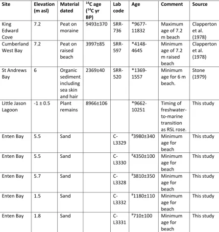
Clapperton et al. (1978) showed that the highest beach they recorded in St Andrews Bay (6-7.2 m) was

cut into a moraine and therefore formed after deglaciation from that moraine. Dates on the

lowermost layer of peat accumulated on top of the till of the equivalent moraine in King Edward Cove

yielded a radiocarbon age of 9493±370 14_{C yr BP (SRR-736), which thus provides a minimum age for}

the moraine. The beach was covered by a layer of peat which yielded a basal age of 3997±85 14_{C yr BP}

(SRR-597). Clapperton et al. (1978) therefore concluded that the highest beach was formed sometime

between 9500 and 4000 14_{C yr BP (equivalent to a calibrated age between 9677 11832 and 4148-4645}

cal yr BP). Calculating the indicative range of a raised marine beach is a challenge (Kelsey, 2015) and

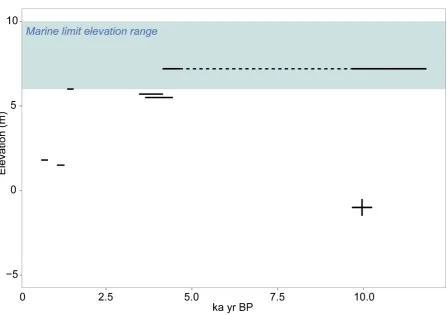
therefore we use the ages from Clapperton et al. (1978) in Figure 3 to constrain the potential

maximum and minimum ages for this feature, but apply a more conservative 6-10 m range for the

(10)

9 Stone (1979) reported a site on the south side of Royal Bay where a series of raised beaches at 6 m asl

extends into a sea-cave system. A fibrous mat of organic sediment including moulted seal skin and

hair yielded a radiocarbon age of 2369±40 14_{C yr BP (SRR-520). This provides a minimum age for the}

6m raised beach found at the back of the cave (Stone, 1979).

In Enten Valley the raised beaches are covered by a sequence of beach foredunes and shadow dunes

where at least seven large beach ridges (E1-7), and several smaller ridges are preserved across a 400

m wide strandplain (Figure 4 and supplementary information). Most of the inland dune sands are

indurated and covered by a thin (0.1-0.3 m) layer of peat, with soil and peat thicknesses generally

increasing inland, suggesting increasing age. Peat accumulations on the dunes are substantially

thinner than on the nearby (near sea level) moraines, which are commonly covered by over a metre

of peat, suggesting the beaches post-date the moraines by some time. New infrared stimulated

luminescence (IRSL) dating indicates that beach crests at 5 m above mean sea level were deposited at

or shortly before the 3810±350 a and 4350±400 a IRSL ages for the foredune basal sand that overlies

the top of the beach crest (further detailed in the supplementary information). Beach crests at <2 m

elevation are covered by dune sands and shadow dunes dated to 1180±110 a and 710±100 a

respectively. These ages imply that RSL fell from 4-5 m shortly after 4000 yr and has been below 1 m

since at least ~1200 yr.

Little Jason Lagoon is a coastal basin in inner Cumberland West Bay (54°11.568'S 36°35.469'W;

detailed in supplementary information). It is near-circular with a narrow entrance and shallow sill at 1

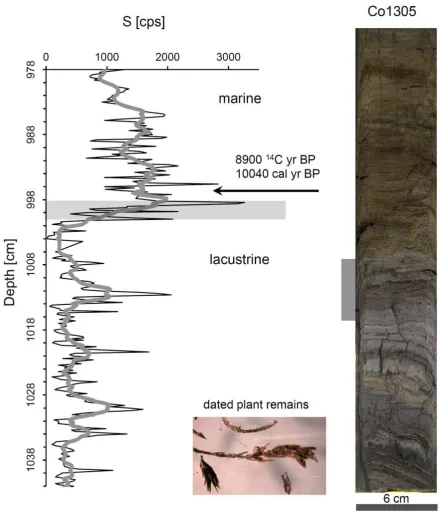
m (±0.5 m) depth. Analysis of a sediment core (Co1305) sampled from within the lagoon has

demonstrated that the sediments record a transition from freshwater (lacustrine) conditions to a

marine lagoon. The transition from a freshwater to marine environment has been identified on the

(11)

10 of isolation (Figure 5). Plant remains from 2 cm above the transition yield a radiocarbon age of

8966±106 14_{C yr BP (9662-10251 cal yr BP) giving a maximum age for the transition from freshwater}

to marine conditions in the basin.

Site Elevation (m asl)

Material dated

14_{C age}

(14_{C yr}

BP)

Lab code

Age Comment Source

King Edward Cove

7.2 Peat on

moraine

9493±370 SRR-736

*9677-11832

Maximum age of 7.2 m beach Clapperton et al. (1978) Cumberland West Bay

7.2 Peat on raised beach

3997±85 SRR-597

*4148-4645

Minimum age of 7.2 m raised beach Clapperton et al. (1978) St Andrews Bay

6 Organic

sediment including sea skin and hair

2369±40 SRR-520

*1369-1557

Minimum age for 6 m beach.

Stone (1979)

Little Jason Lagoon

-1 ± 0.5 Plant remains

8966±106

*9662-10251

Timing of freshwater-to-marine transition as RSL rose.

This study

Enten Bay 5.5 Sand

C-L3329

#_{3980±340 Minimum} age for beach

This study

Enten Bay 5.5 Sand

C-L3330

This study

Enten Bay 5.7 Sand

C-L3328

This study

Enten Bay 1.5 Sand

C-L3332

This study

Enten Bay 1.8 Sand

C-L3331

#_710±100 _Minimum age for beach

[image:11.595.74.522.165.641.2]

This study

Table 1 - Dated relative sea level constraints from South Georgia.

* (cal yr BP), radiocarbon ages calibrated using CALIB v.7.1 (http://calib.qub.ac.uk/) (Stuiver and

Reimer, 1993). Reported calibrated ages are the 2-sigma ranges, using the SH13 curve (Hogg et al.,

2013). Marine reservoir correction for seal hair taken as 750 yr (Sugden and John, 1973).

(12)

11 The dated RSL data points are compiled in Figure 3 to provide a series of constraints against which the

GIA model results can be compared, though the main constraint is the elevation of the ~6-10 m marine

limit.

Glacial isostatic adjustment modelling

Modelling of the solid earth response and resulting RSL changes to test the proposed maximum and

minimum ice scenarios is done using ALMA (Spada, 2008), which is specifically suitable for GIA regional

modelling and high spatial resolutions. ALMA implements the Post Widder formula and computes the

Love numbers for a spherical self-gravitating, layered, incompressible Earth model with Maxwell

rheology. The viscosity profile is a volume- P (2004) Earth model

VM2: lower mantle viscosity 2.7 x 1021_{Pa s and upper mantle 0.5 x 10}21_{Pa s. The lithosphere is elastic}

with a thickness of 90 km. There is no direct evidence for a low viscosity mantle at this location and

this allows us to integrate the ICE-5G (VM2) solutions computed in SELEN (Spada et al., 2012; Spada

and Stocchi, 2007) for far-field RSL changes driven by changes in the global ice sheets from their LGM

maximum (Figure 6). We do not use ICE-6G model (Argus et al., 2014; Peltier et al., 2015) at this time

due to uncertainties surrounding the Antarctic Peninsula component (Purcell et al., 2016), which due

to its proximity to South Georgia may have implication for our results. Figure 6 shows that South

Georgia experiences relatively minor far-field isostatic effects and the resulting RSL signal from the

global model is primarily due to changes in total ocean volume (often termed the eustatic function)

(Figure 6B). This global-model RSL curve is added to our local predictions of RSL changes driven by our

South Georgia ice-load models. It must be noted that the ICE-5G (VM2) model of Peltier (2004)

includes a compressible Earth structure, which may result in ~0.1 mm yr-1_{error when computed in our}

(13)

12 Our modelling approach seeks to test the two different LGM hypotheses but does not aim to

accurately simulate the past ice cap topography due to the limited palaeo-glaciological constraints.

F provide a simple but robust test between

extensive (whole continental shelf occupied by ice) and restricted (ice within the island coastline)

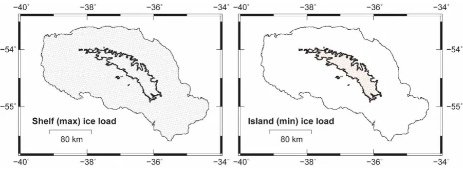
ice-load models. The extensive shelf model includes 2315 4.74 km diameter discs, with the restricted

island-only ice load comprising 202 discs (Figure 7). Using discs has been a long adopted method for

gridding ice load (e.g. Tushingham and Peltier, 1991) to minimise overlap and gaps. The model is

computed with 15,000 spherical harmonics to allow for the small load diameter (after Bevis et al.,

2016). Increasing the number of discs, i.e. decreasing their diameter, increases the computational

intensity at no benefit to the results (Bevis et al., 2016). We test different ice-model thicknesses for

each maximum and minimum ice scenario in order to understand the sensitivity of our model output

to local thickness changes. We develop 8 key scenarios which allow us to test the maximum and

minimum load hypotheses, applying ice loads at 1 k yr time-steps in different combinations (Table 2),

partly constrained by the geomorphological evidence discussed above. Ice-load histories are given

relative to present from 22 to 0 ka, with a constant load from 71 ka to the LGM in order to allow

reasonable equilibration of the ice load. In each of the extensive (shelf) or restricted (island) ice

models all the discs have the same stepwise ice-load history, and all ice models include a 100 m thick

load for the island-only discs at 4-3 ka and 1-0 ka to allow for Neoglacial and recent ice advances

(Bentley et al., 2007; Hall, 2009). The model does not allow for underlying topographic variations and

therefore the stated values are the uniform ice thickness, not the height of the ice surface with respect

to the underlying topography. The limited glaciological evidence for the LGM ice-cap behaviour on

South Georgia means that it is not currently feasible to develop spatially variable time-retreating

ice-load histories. The model outputs are computed for 12 key locations (Figure 1) including four GPS

(14)

13 Model

number Description

Island (restricted) ice load

Shelf (extensive) ice load

1 Restricted, thin, island only load 22-12 ka: 100 m - 2 Restricted, thick, island only load 22-12 ka: 1000 m -

3 Restricted, very thick, island only load 22-21 ka: 3000 m

21-12 ka: 1000 m -

4 Thick, LGM shelf load, post-LGM small, thin, island only load

22-21 ka: 1000 m 22-12 ka: 100 m

22-21 ka: 1000 m

5 Extensive, thin shelf load, until 15 ka 22-15 ka: 100 m 22-15 ka: 100 m 6 Extensive, thick shelf load, until 18 ka 22-18 ka: 1000 m 22-18 ka: 1000 m 7 Extensive, thick shelf load, until 15 ka 22-15 ka: 1000 m 22-15 ka: 1000 m 8 Extensive, thick shelf load, until 12 ka 22-12 ka: 1000 m 22-12 ka: 1000 m Table 2 South Georgia ice model scenarios used in ALMA

Results

The results of the ALMA RSL curves for the 12 observer locations on South Georgia, combined with

the SELEN modelled ICE-5G RSL curve (Figure 6), are plotted in Figure 8 and compared with the RSL

data and marine limit elevations. Fit with the data is assessed visually as the restricted number of

available RSL data points and their marine limiting nature means a statistical assessment is not viable.

Due to the simplicity of the ice model there is very little spatial variation between the 12 modelled

observer locations during the Holocene, so the results are not plotted by separate colours in Figure 8

and are discussed for all the modelled South Georgia sites collectively. All the model outputs predict

a rise from a post-LGM lowstand, with the pre-Holocene part of the RSL curves tracking the general

RSL rise of the ICE-5G global modelled curve in Figure 6B.

The restricted ice-load models, which only contain ice on the island (models 1-3), as well as model 4

which has 1000 m thick ice on the shelf until 21 ka followed by restricted island-only ice, do not predict

a Holocene highstand (Figure 8). The modelled RSL curves are dominated by the global GIA signal with

the highest modelled sea level occurring at the present day. The field data provides strong evidence

for a period of post-LGM sea level higher than present, which suggests that the restricted ice models

do not contain enough local mass to result in a solid earth deformation to fit the geomorphological

[image:14.595.73.536.71.248.2]

(15)

14 The extensive shelf-edge model with only 100 m of ice (model 5) also does not predict RSL above

present (Figure 8). It is only in the load scenarios where the ice thickness is increased to 1000 m in

extensive models 6-8 do the outputs predict a period of RSL above present (Figure 8 and S6),

demonstrating the importance of local GIA overprinting the far-field derived RSL. In model 6 (18 ka

deglaciation) a 0.8 m highstand occurs at 5 ka, and in model 7 (15 ka deglaciation) a 4.2 m highstand

occurs at 9 ka. Model 8 (12 ka deglaciation) has a double peaked highstand of 15.9 m at 13 ka, followed

by a second of 13.0 m at 9 ka. This is the only model which predicts sea level far above the ca. 6-10 m

marine limit implied by the geomorphological sea-level data (Figure 3). The timing of deglaciation in

model 8 is also much too late to fit with the evidence of the onset of ice-free conditions at Tønsberg

Point (Rosqvist et al., 1999). The output provides a useful maximum load end-member, but we are

able to reject this solution. The extensive thick shelf-edge ice loads in models 6 and 7 provide the

closest fit with the geomorphological sea-level data, with the higher highstand in model 7 of ca. 4 m,

nearest in elevation to the measured marine limit, suggesting this is the optimum scenario. Crucially

we find that an extensive thick model with relatively early deglaciation can simulate a highstand of

similar timing and magnitude as the field data.

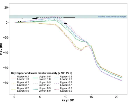
To test the sensitivity of the results with respect to changes in the rheology of the Earth, we combine

the deglaciation model 7 with different viscosity profiles (Figure 9), keeping fixed the lithospheric

thickness at the ICE-5G(VM2) value of 90 km since we know that this parameter plays a minor role in

the GIA response (see Stocchi and Spada, 2009). It should be noted that the results in Figure 9 have

mainly a qualitative character, since modifying the VM2 viscosity profile alters the agreement of the

ICE-5G (VM2) predictions with the set of global Holocene RSL curves used to calibrate it. As pointed

out by Tamisiea (2011), more realistic GIA estimates could be obtained by simultaneously varying the

D E

into account, which is beyond the scope of this work. Due to the relatively small sensitivity of the RSL

(16)

15 Figure 9. The ranges for the local upper mantle viscosity and the lower mantle viscosity are 0.2 to 0.8

x 1021_{Pa s and 1.0 to 5.0 x 10}21_{Pa s, respectively. It is apparent that when the ICE-5G(VM2) upper}

mantle viscosity is used (0.5 x 1021_{Pa s), a satisfactory fit with the data is obtained for all the lower}

mantle viscosities considered (the insensitivity to lower mantle viscosity is explained by the relatively

small size of the ice load). The misfit increases when the upper mantle viscosity is too low (0.2 x 1021

Pa s, which implies a fast relaxation) or too high (0.8 x 1021_{Pa s, which enhances the amplitude of the}

highstand) compared to the VM2 value.

Discussion

Testing models of LGM ice extent on South Georgia

The results of the GIA modelling presented in this paper, when compared to marine limit and RSL data,

support the extensive glaciation hypothesis where LGM ice extends to the continental shelf edge

(Clapperton et al., 1989; Graham et al., 2008; Sugden and Clapperton, 1977). Even with an extreme

ice thickness of 3000 m (which is higher than the elevation of the highest summit, Mount Paget, and

does not allow for underlying topography) in the restricted island-only model 3, the GIA outputs

cannot produce a highstand to produce a ca. 6-10 m marine limit. Therefore, based upon GIA

modelling, it seems unlikely that the restricted glaciation model of Bentley et al. (2007) is valid. The

model (7) which provides the best fit with the data, suggests deglaciation of the shelf at ca. 15 ka BP.

This is potentially ca. 4 ka later than suggested by the onset of lake sedimentation at Tønsberg Point

(Rosqvist et al., 1999). A limitation of our approach is the lack of a spatially variable load and

accounting for the underlying topography. It remains possible to fit the RSL data with an extensive ice

cap model together with a spatially and temporally variable deglacial history to accommodate early

deglaciation at Tønsberg, but this is beyond the scope of this study. This could be revisited when

(17)

16 The results of an extensive LGM ice cap on South Georgia requires the reinterpretation of existing

research. As proposed by Graham et al. (2008) this implies that terrestrial and fjord moraines mapped

by Bentley et al. (2007) and Hodgson et al. (2014a) are in fact either retreat, stillstand or readvance

margins of a post-LGM ice cap, formed subsequently to the maximum extension of the ice onto the

continental shelf. The moraines mapped by Graham et al. (2008) at the shelf edge are therefore most

likely to be LGM in age and a programme of offshore dating could establish this. Both Sugden and

Clapperton (1977) and Hodgson et al. (2014a) suggest that the offshore evidence of glacial erosion

may be from a previous Pleistocene extensive glaciation. However, we are able to produce modelled

elevations of RSL which fit with the geomorphological data based upon the simplest explanation of a

large LGM ice cap, avoiding the complication of multiple phases of GIA through multiple

glacial-interglacial cycles.

Our results also have implications for the long-term evolution of the island. Given the difficulty of

producing substantive highstands in the GIA models, even with a very substantial extensive ice cap it

seems unlikely that the rock platforms could have been formed at their current elevations (20-50m)

due to GIA alone. This is particularly apparent when their size is taken into account as they would

potentially have needed substantial periods of time to be eroded. It seems more likely that they may

have formed during one or more previous interglacial highstands, implying long-term uplift of the

island. We also cannot rule out that the platforms are entirely pre-glacial. Long-term uplift is

consistent with thermochronological data that suggest the island may have seen significant

exhumation since 10 Ma (Carter et al., 2014). Given that the platforms have survived at least one

glaciation, possibly several, we suggest that the LGM ice cap on South Georgia was not particularly

efficient at eroding pre-existing deposits (e.g. preserved beach material up to 52 m asl) or the higher

rock platforms. The non-erosion of more extensive raised beaches and enclosed marine fauna on

Prince Karls Forland on western Svalbard (Evans and Rea, 2005; Landvik et al., 2005; Mangerud et al.,

(18)

17 overrun by glacier ice, constitute examples of similarly ineffective glacial erosion of pre-existing

deposits at low elevations around the margins of an ice sheet-covered archipelago similar to South

Georgia. Whether, like the Svalbard and Baffin Island examples, the survival of raised marine features

was related to cold-based ice sheet marginal conditions or just localized ineffective erosion cannot be

determined at this stage.

Ongoing land-level change on South Georgia

The available RSL data that constrains our GIA models is limited and precludes the development of a

spatially variable ice load model. Aside from collecting further geomorphological evidence of RSL

change, there may be potential to further constrain the spatial and temporal ice history of future

models using instrumental data based upon the spatial pattern of modern rates of land-level change.

The first global navigation satellite system (GNSS) station in South Georgia was installed on Brown

Mountain (station: KEPA), King Edward Point in February 2013 with the aim of providing a reference

point for the King Edward Point tide gauge and constrain tectonic motion of South Georgia (Teferle,

pers. comm.). Three additional stations were installed in October 2014 at northern (SOG2), southern

(SOG1) and eastern (SOG3) locations in South Georgia (Dalziel, pers. comm.). The short duration of

the records means they are not yet suitable to use as constraints in this study, but a network of GPS

locations providing detailed information as to the spatial pattern of present day rates of land-level

change may help resolve model outputs further and allow for more complex ice load histories to be

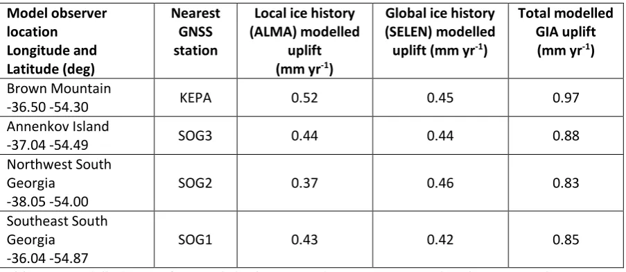
tested in the absence of geomorphological constraints. In the meantime, using the ALMA outputs of

the local ice cap in Model 7 (Figure 8) and outputs from SELEN (Figure 6), we are able to provide

estimates of present rates of vertical uplift at the four GPS sites as explained by the local and global

modelled GIA (Table 3). Differences between these estimates and measured vertical rates may be

(19)

18 Model observer location Longitude and Latitude (deg) Nearest GNSS station

Local ice history (ALMA) modelled

uplift (mm yr-1₎

Global ice history (SELEN) modelled uplift (mm yr-1₎

Total modelled GIA uplift (mm yr-1₎

Brown Mountain

-36.50 -54.30 KEPA 0.52 0.45 0.97

Annenkov Island

-37.04 -54.49 SOG3 0.44 0.44 0.88

Northwest South Georgia

-38.05 -54.00

SOG2 0.37 0.46 0.83

Southeast South Georgia

-36.04 -54.87

SOG1 0.43 0.42 0.85

Table 3 Modelled rate of vertical displacement due to post-LGM glacial isostatic adjustment as

computed by the models detailed in this paper at the four GPS locations on South Georgia. Locations

from N. Teferle, (pers. comm.) and Dalziel, (pers. comm.). More information is available at

https://www.unavco.org/data/gps-gnss/gps-gnss.html

Wider implications of an extensive LGM ice cap on South Georgia

The suggestion of an extensive thick ice cap on South Georgia has implications for other sub-Antarctic

islands, on which limited geomorphological evidence is recorded, but where there exists similar

debate about the extent of Quaternary glaciation(s) (Hodgson et al., 2014b; Sugden and Clapperton,

1977). If a large LGM ice cap existed in South Georgia then there is potential for the same to have

occurred on other sub-Antarctic islands within a similar climatic context e.g. Kerguelen, and also fits

with other models of extensive LGM ice proposed for Heard, Bouvet and the South Orkney Islands

(Hodgson et al., 2014b). The presence of an extensive LGM ice cap that reached the continental shelf

edge around South Georgia suggests affinity with West Antarctica and the Antarctica Peninsula, which

also experienced the most extensive glaciation at the LGM, rather than with Patagonia where the

greatest glacial extents were earlier in the Quaternary (Darvill et al., 2015). Our model results suggests

that deglaciation on South Georgia occurred ca. 15 ka, which fits with geomorphological data from the

[image:19.595.73.525.70.266.2]

(20)

19 well as dates of the onset of peat formation and lake sedimentation at other sub-Antarctic islands,

including Kerguelen, Auckland and Campbell, around this time (Hodgson et al., 2014b).

Our conclusion of an extensive ice cap extending to the shelf edge would imply that if there were any

biological refugia around South Georgia, they must have been relatively localised and restricted to the

outermost shelf and any potential nunataks. Our model is not spatially variable and so we are unable

to determine the locations of these refugia using current datasets. Our fits with a recent assessment

of the seabed biodiversity around South Georgia which concludes that most of the shelf is still

undergoing recolonization following glacial retreat (Barnes et al., 2016).

The approach presented here, to use GIA modelling and associated RSL data to differentiate between

opposing models of ice extent, may also be applied in other locations where similar debates exist, e.g.

Iceland (Brader, 2015). The order-of-magnitude difference of the modelled RSL changes as a result of

the maximum versus minimum ice extent models, means this approach is able to provide a first order

test of the hypotheses without the need for detailed glacial histories. This is particularly valuable

where offshore data is limited or lacks a chronology. However, not all current GIA models are designed

to work at the sufficiently high enough number of spherical harmonics required to resolve differences

between relatively small ice loads. Thus, a bespoke solution, such as used here with the flexible code

in SELEN and ALMA (Spada, 2008; Spada et al., 2012; Spada and Stocchi, 2007), may be required.

Conclusions

We conclude from our GIA modelling and constrained by a newly-compiled RSL dataset, that the LGM

glaciation of South Georgia was extensive and extended to the shelf edge at a time when the island

was covered by thick (>1000 m) ice. Deglaciation occurred relatively early, indeed our best fit model

suggests substantial deglaciation by ca. 15 ka BP, although independent data suggests this may have

(21)

20 ice cap and the date and timing of deglaciation in order to allow the development of a more

sophisticated and spatially-variable ice model. This will also require the collection of additional sea

level index points to constrain the modelled outputs, and comparison of GPS-derived uplift rates to

(22)

21 Acknowledgements

We thank the Royal Scottish Geographical Society (RSGS), Carnegie Trust for the Universities of

Scotland, and National Geographic for fieldwork support and to the members of the RSGS Scotia

expedition for field assistance. We are also grateful to the Government of South Georgia and the South

Sandwich Islands for permits and assistance in our work. This paper has benefited from discussions

with Alastair Graham (who also provided Figure 1A), Dominic Hodgson and Pippa Whitehouse,

members of PALSEA2 (an INQUA International Focus Group and a PAGES working group) and the

Quaternary Research Association Sea Level and Coastal Change (SLaCC) working group. G.S. is funded

by Programma Nazionale di Ricerche in Antartide (PNRA) 2013/B2.06 (CUP D32I14000230005).

(23)

(24)

23 Figure 1: Location Maps of South Georgia. (a) Summary map of bathymetry and geomorphology of South Georgia and its surrounding continental shelf (from

Graham et al., 2008). Fault (dot-dash line) inferred from onshore expression of strike-strike fault (solid line) in the south east of the island. TMF, trough mouth

fan. (b) Location Map of South Georgia. All place names are taken from map: South Georgia 1:200k, British Antarctic Survey Misc Sheet 12A and 12B. Red

crosses mark locations of model predictions, including GPS sites in Table 3). (c) Raised beaches around South Georgia. Dots are scaled according to size and

the elevation (m asl) of the highest beach or marine limit is shown beside symbol. (d) Rock platforms around South Georgia. Dots are scaled according to size

(25)

[image:25.595.73.525.76.706.2]

24 Figure 2: Photographs of examples of the coastal geomorphology of South Georgia. A) Upper (7 m

(26)

25 in Cumberland Bay, C) Raised beaches at Moraine Fjord, and D) Raised beaches at Sandebugten, Barff

Peninsula. E) Rock platforms at Stromness Bay, F) Rock platform at Tønsberg Peninsula, G) Rock

[image:26.595.76.524.171.486.2]

platforms at Carlita Bay and H) Rock platform at Tønsberg Peninsula.

Figure 3: Relative sea-level data for South Georgia (from Table 1). Blue band gives 6-10 m typical range

of highest raised beaches mapped on the island (references in text and supplementary information

Tables S1 and S2). Dotted line joins the maximum and minimum ages of the formation of the raised

(27)

[image:27.595.82.515.73.321.2]

26 Figure 4: Topographic and geologic cross section through the centre of Enten Valley from Cumberland

Fjord (left) ~400 m west to a small beach-dammed lake (right). Luminescence ages are shown with

field/lab codes (detailed in Table S3), while major beach ridges are labelled E1-7, though E5 is not well

(28)

[image:28.595.76.517.67.582.2]

27 Figure 5: Sulphur counts (black line 2mm and grey line 2cm running average) obtained with an XRF

core scanner for core Co1305 (1042 to 978 cm depth) from Little Jason Lagoon. Line scan image of the

core section containing the lacustrine/marine transition. Grey bar indicates the position of increase in

(29)

[image:29.595.78.527.72.278.2]

28 Figure 6: A: Map of present day rates of relative sea-level change modelled in SELEN using ICE-5G and

a VM2 average viscosity (details on Figure). B: Relative sea-level changes due to global GIA at South

Georgia (dotted line) are similar to the global (eustatic) changes in ice volume in ICE-5G (solid line).

Figure 7: Disc ice loads extents in ALMA for the extensive shelf (maximum) and restricted (minimum)

[image:29.595.72.523.399.565.2]

(30)

(31)

30 Figure 8: Modelled relative sea-level changes using the 8 ice models detailed in Table 2 plotted against

data from Figure 3 (note blue band of marine limit in Figure 3 shown as dotted line here for simplicity).

Relative sea-level curves are a combination of the ALMA modelled outputs in response to the ice

thickness changes plotted in each graph (colours correspond to the ice models in Figure 7) combined

with the South Georgia SELEN global model relative sea level in Figure 6B. Note, output for all the 12

observer locations are plotted in a single colour as they are so similar it is not possible to visually

[image:31.595.75.525.275.637.2]

separate them.

Figure 9: Modelled relative sea-level changes at the Brown Mountain GPS station using ice model 7

(detailed in Table 2) and a range of upper and lower mantle viscosities (x 1021_{Pa s) plotted against}

relative sea level data from Figure 3. Earth model used in outputs in Figure 8 shown by grey dotted

(32)

31 References

Adie, R.J., 1964. Sea level changes in the Scotia Arc and Graham Land, in: Adie, R.J. (Ed.), Antarctic Geology. North-Holland Publishing Company, Amsterdam, pp. 27-32.

Argus, D.F., Peltier, W.R., Drummond, R., Moore, A.W., 2014. The Antarctica component of postglacial rebound model ICE-6G_C (VM5a) based on GPS positioning, exposure age dating of ice thicknesses, and relative sea level histories. Geophysical Journal International 198, 537-563.

Barnes, D.K.A., Hodgson, D.A., Convey, P., Allen, C.S., Clarke, A., 2006. Incursion and excursion of Antarctic biota: past, present and future. Global Ecology and Biogeography 15, 121-142.

Barnes, D.K.A., Sands, C.J., Hogg, O.T., Robinson, B.J.O., Downey, R.V., Smith, J.A., 2016. Biodiversity signature of the Last Glacial Maximum at South Georgia, Southern Ocean. Journal of Biogeography, n/a-n/a.

Bentley, M.J., Evans, D.J.A., Fogwill, C.J., Hansom, J.D., Sugden, D.E., Kubik, P.W., 2007. Glacial geomorphology and chronology of deglaciation, South Georgia, sub-Antarctic. Quaternary Science Reviews 26, 644-677.

Bentley, M.J., Ó Cofaigh, C., Anderson, J.B., Conway, H., Davies, B., Graham, A.G.C., Hillenbrand, C.-D., Hodgson, D.A., Jamieson, S.S.R., Larter, R.D., Mackintosh, A., Smith, J.A., Verleyen, E., Ackert, R.P., Bart, P.J., Berg, S., Brunstein, D., Canals, M., Colhoun, E.A., Crosta, X., Dickens, W.A., Domack, E., Dowdeswell, J.A., Dunbar, R., Ehrmann, W., Evans, J., Favier, V., Fink, D., Fogwill, C.J., Glasser, N.F., Gohl, K., Golledge, N.R., Goodwin, I., Gore, D.B., Greenwood, S.L., Hall, B.L., Hall, K., Hedding, D.W., Hein, A.S., Hocking, E.P., Jakobsson, M., Johnson, J.S., Jomelli, V., Jones, R.S., Klages, J.P., Kristoffersen, Y., Kuhn, G., Leventer, A., Licht, K., Lilly, K., Lindow, J., Livingstone, S.J., Massé, G., McGlone, M.S., McKay, R.M., Melles, M., Miura, H., Mulvaney, R., Nel, W., Nitsche, F.O., O'Brien, P.E., Post, A.L., Roberts, S.J., Saunders, K.M., Selkirk, P.M., Simms, A.R., Spiegel, C., Stolldorf, T.D., Sugden, D.E., van der Putten, N., van Ommen, T., Verfaillie, D., Vyverman, W., Wagner, B., White, D.A., Witus, A.E., Zwartz, D., 2014. A community-based geological reconstruction of Antarctic Ice Sheet deglaciation since the Last Glacial Maximum. Quaternary Science Reviews 100, 1-9.

Bevis, M., Melini, D., Spada, G., 2016. On computing the geoelastic response to a disk load. Geophysical Journal International 205, 1804-1812.

Brader, M.D., 2015. Postglacial relative sea-level changes and the deglaciation of northwest Iceland, Department of Geography. Durham University.

Carter, A., Curtis, M., Schwanethal, J., 2014. Cenozoic tectonic history of the South Georgia microcontinent and potential as a barrier to Pacific-Atlantic through flow. Geology 42, 299-302. Clapperton, C.M., 1971. Geomorphology of the Stromness Bay-Cumberland Bay area, South Georgia, British Antarctic Survey Scientific reports No. 70. Natural Environment Research Council.

Clapperton, C.M., Sugden, D.E., Birnie, J., Wilson, M.J., 1989. Late-glacial and Holocene glacier fluctuations and environmental change on South Georgia, Southern Ocean. Quaternary Research 31, 210-228.

Clapperton, C.M., Sugden, D.E., Birnie, R.V., Hansom, J.D., Thom, G., 1978. Glacier fluctuations in South Georgia and comparison with other island groups in the Scotia Sea, in: Bakker, V.Z. (Ed.), Antarctic Glacial History and World Palaeoenvironments, Balkema Rotterdam.

Cook, A.J., Poncet, S., Cooper, A.P.R., Herbert, D.J., Christie, D., 2010. Glacier retreat on South Georgia and implications for the spread of rats. Antarctic Science 22, 255-263.

Darvill, C.M., Bentley, M.J., Stokes, C.R., Hein, A.S., Rodés, Á., 2015. Extensive MIS 3 glaciation in southernmost Patagonia revealed by cosmogenic nuclide dating of outwash sediments. Earth and Planetary Science Letters 429, 157-169.

Davis, P.T., Briner, J.P., Coulthard, R.D., Finkel, R.W., Miller, G.H., 2006. Preservation of Arctic landscapes overridden by cold-based ice sheets. Quaternary Research 65, 156-163.

(33)

32 Gordon, J.E., Haynes, V.M., Hubbard, A., 2008. Recent glacier changes and climate trends on South Georgia. Global and Planetary Change 60, 72-84.

Gordon, J.E., Timmis, R.J., 1992. Glacier fluctuations on South Georgia during the 1970s and early 1980s. Antarctic Science 4, 215-226.

Graham, A.G.C., Fretwell, P.T., Larter, R.D., Hodgson, D.A., Wilson, C.K., Tate, A.J., Morris, P., 2008. A new bathymetric compilation highlighting extensive paleo ice sheet drainage on the continental shelf, South Georgia, sub-Antarctica. Geochemistry, Geophysics, Geosystems 9, n/a-n/a.

G J W T “ G M F

Ferguson, D. (Ed.), Geological Observations in South Georgia, Transactions of the Royal Society of Edinburgh, pp. 814-816.

Hall, B.L., 2009. Holocene glacial history of Antarctica and the sub-Antarctic islands. Quaternary Science Reviews 28, 2213-2230.

Hansom, J.D., 1979. Beach Form and Process Variation in South Georgia, a sub-Antarctic Island. University of Aberdeen, Unpublished PhD thesis.

Hodgson, D.A., Graham, A.G.C., Griffiths, H.J., Roberts, S.J., Cofaigh, C.Ó., Bentley, M.J., Evans, D.J.A., 2014a. Glacial history of sub-Antarctic South Georgia based on the submarine geomorphology of its fjords. Quaternary Science Reviews 89, 129-147.

Hodgson, D.A., Graham, A.G.C., Roberts, S.J., Bentley, M.J., Cofaigh, C.Ó., Verleyen, E., Vyverman, W., Jomelli, V., Favier, V., Brunstein, D., Verfaillie, D., Colhoun, E.A., Saunders, K.M., Selkirk, P.M., Mackintosh, A., Hedding, D.W., Nel, W., Hall, K., McGlone, M.S., Van der Putten, N., Dickens, W.A., Smith, J.A., 2014b. Terrestrial and submarine evidence for the extent and timing of the Last Glacial Maximum and the onset of deglaciation on the maritime-Antarctic and sub-Antarctic islands. Quaternary Science Reviews 100, 137-158.

Hogg, A.G., Hua, Q., Blackwell, P.G., Niu, M., Buck, C.E., Guilderson, T.P., Heaton, T.J., Palmer, J.G., Reimer, P.J., Reimer, R.W., Turney, C.S.M., Zimmerman, S.R.H., 2013. SHCal13 Southern Hemisphere Calibration, 0 50,000 Years cal BP.

Hogg, O.T., Barnes, D.K., Griffiths, H.J., 2011. Highly diverse, poorly studied and uniquely threatened by climate change: an assessment of marine biodiversity on South Georgia's continental shelf. Plos One 6, e19795.

Kelsey, H.M., 2015. Geomorphological indicators of past sea levels, Handbook of Sea-Level Research. John Wiley & Sons, Ltd, pp. 66-82.

Landvik, J.Y., Ingolfsson, O., Mienert, J., Lehman, S.J., Solheim, A., Elverhoi, A., Ottesen, D., 2005. Rethinking Late Weichselian ice-sheet dynamics in coastal NW Svalbard. Boreas 34, 7-24.

Mangerud, J., Jansen, E., Landvik, J.Y., 1996. Late Cenozoic history of the Scandinavian and Barents Sea ice sheets. Global and Planetary Change 12, 11-26.

Miller, G.H., Sejrup, H.P., Lehman, S.J., Forman, S.L., 1989. Glacial history and marine environmental change during the last interglacial-glacial cycle, western Spitsbergen, Svalbard. Boreas 18, 273-296. Peltier, W.R., 2004. Global glacial isostasy and the surface of the ice-age earth: The ICE-5G (VM2) model and GRACE. Annual Review of Earth and Planetary Sciences 32, 111-149.

Peltier, W.R., Argus, D.F., Drummond, R., 2015. Space geodesy constrains ice age terminal deglaciation: The global ICE-6G_C (VM5a) model. Journal of Geophysical Research: Solid Earth 120, 450-487.

Purcell, A., Tregoning, P., Dehecq, A., 2016. An assessment of the ICE6G_C(VM5a) glacial isostatic adjustment model. Journal of Geophysical Research: Solid Earth 121, 3939-3950.

Rosqvist, G.C., Rietti-Shati, M., Shemesh, A., 1999. Late glacial to middle Holocene climatic record of lacustrine biogenic silica oxygen isotopes from a Southern Ocean island. Geology 27, 967-970. Smith, J., 1960. Glacier problems in South Georgia. Journal of Glaciology 705-714.

Spada, G., 2008. ALMA, a Fortran program for computing the viscoelastic Love numbers of a spherically symmetric planet. Computers & Geosciences 34, 667-687.

(34)

33

“ G “ P “ELEN A F

-Computers & Geosciences 33, 538-562.

Stocchi, P., Spada, G., 2009. Influence of glacial isostatic adjustment upon current sea level variations in the Mediterranean. Tectonophysics 474, 56-68.

Stone, P., 1974. Physiography of the North-east coast of South Georgia, British Antarctic Survey Bulletin, pp. 17-36.

Stone, P., 1976. Raised marine and glacial features of the Cooper Bay-Wirik Bay area, South Georgia, British Antarctic Survey Bulletin. 44, 47-56.

Stone, P., 1979. Raised Marine features on the south side of Royal Bay, South Georgia, British Antarctic Survey Bulletin, pp. 137-141.

Stuiver, M., Reimer, P.J., 1993. Extended 14C database and revised CALIB 3.0 radiocarbon calibration program. Radiocarbon 35, 215-230.

Sugden, D.E., Clapperton, C.M., 1977. The maximum ice extent on island groups in the Scotia sea, Antarctica. Quaternary Research 7, 268-282.

Sugden, D.T., John, B.S., 1973. The ages of glacier fluctuations in the South Shetland Islands, Antarctica, Palaeoecology of Africa, the Surrounding Islands and Antarctica. Balkema, Cape Town, pp. 141-159.

Tamisiea, M.E., 2011. Ongoing glacial isostatic contributions to observations of sea level change. Geophysical Journal International 186, 1036-1044.

Thatje, S., Hillenbrand, C.-D., Mackensen, A., Larter, R., 2008. Life Hung by a Thread: Endurance of Antarctic Fauna in Glacial Periods. Ecology 89, 682-692.

(35)

1

Testing models of ice cap extent, South Georgia, sub-Antarctic.

Quaternary Science Reviews

Barlow, N.L.M.1,2*_{, Bentley, M.J.}1_{, Spada, G.}3_{, Evans, D.J.A.}1_{, Hansom, J.D.}4_{, Brader, M.D.}1_{, White, D.A.}5_,

Zander, A.6_{, Berg, S.}7

1_{Department of Geography, Durham University, South Road, Durham, DH1 3LE, UK}

2_{School of Earth and Environment, University of Leeds, Leeds, LS2 9JT, UK}

3_{Dipartimento di Scienze Pure e Applicate (DiSPeA) Urbino University ''Carlo Bo'', Urbino, Italy}

4_{School of Geographical and Earth Sciences, University of Glasgow, Glasgow, G12 8QQ, UK}

5_{Institute for Applied Ecology, University of Canberra, Canberra, ACT 2617, Australia.}

6_{Institute of Geography, University of Cologne, Albertus-Magnus-Platz, 50923 Cologne, Germany}

7 _{Institute of Geology and Mineralogy, University of Cologne, Zülpicher Str. 49a, 50674 Cologne,} Germany

* Corresponding author: [email protected] +44 113 343 3761

(36)

2 Supplementary information

Database of raised beaches and rock platforms (shown in main text Figure 1): p3-7

Table S1: Raised beach locations and elevations in South Georgia. For references see main text.

Table S2: Rock platform locations and elevations in South Georgia. For references see main text.

Reports of Enten beach samples and IRSL dating: p8-15

Figure S1: Enten Valley strandplain and IRSL sample locations

Figure S2: Site photographs for luminescence samples.

Tables S3-S4 and Figures S3-S4: Infra-red stimulated luminescence (IRSL) dating results

Report of Little Jason Lagoon Core : p16-18

Figure S5: Site photograph of Little Jason Lagoon

GIA modelling : p19

(37)

3 Table S1 Raised beaches

No. Location Latitude Longitude Elevation (m) Source

1 Hamilton Bay -54.79412 -35.90121 7 Hansom, 1979

2 Cooper Bay -54.792077 -35.814659 5 This study

3 Cooper Bay -54.789154 -35.818142 4 This study

4 Cooper Bay -54.781818 -35.813023 4 Stone, 1976

5 Wirik Bay -54.751709 -35.845035 5 Stone, 1976

6 Wirik Bay -54.743355 -35.859795 3 Stone, 1976

7 Iris Bay -54.696988 -35.930618 9 Stone, 1976

8 Gold Harbour -54.617414 -35.938819 9 Stone, 1974

9 Bjornstadt Bay -54.590954 -35.924955 7 Stone, 1974

10 Royal Bay -54.577820 -35.979003 3 Stone, 1974

11 Royal Bay -54.567385 -36.016540 8 Stone, 1974

12 Little Moltke Habour, Royal Bay -54.548743 -36.105710 4 This study

13 Moltke Harbour, Royal Bay -54.523322 -36.086989 7 This study

14 Moltke Harbour, Royal Bay -54.522224 -36.087810 5 This study

15 Molte Harbour, Royal Bay -54.521123 -36.087053 6 Stone, 1974

16 Molte Harbour, Royal Bay -54.518153 -36.040411 7 Stone, 1974

17 Sacramento Bight -54.501913 -36.026061 3 Stone, 1974

18 Kelp Bay, St Andrews Bay -54.466449 -36.116617 5 Stone, 1974

19 Doris Bay, St Andrews Bay -54.460396 -36.151381

7 Gordon and Hansom, 1986; Stone, 1974

20 Cape Douglas, Barff Peninsula -54.261184 -36.346232 7 This study

21 Barff Point, Barff Peninsula -54.245932 -36.400931 6 Stone, 1974

22 Cumberland East Bay -54.300032 -36.373914 7 This study

23 Sandebugten, Cumberland East Bay -54.311321 -36.355364 9 Stone, 1974

24 Cumberland East Bay -54.326764 -36.352630 6 Stone, 1974

[image:37.842.74.749.97.523.2]

(38)

4

31 Moraine Fjord, Cumberland East Bay -54.316307 -36.446042 2 This study

32 Moraine Fjord, Cumberland East Bay -54.325379 -36.456353 2 This study

33 King Edward Cove, Cumberland East Bay -54.292298 -36.492794 5 This study

34 Ocean Harbour, Barff Peninsula -54.332568 -36.259238 7 Stone, 1974

35 Godthul, Barff Peninsula -54.292020 -36.307719 3 Stone, 1974

36 Cumberland West Bay -54.270507 -36.591188 5 This study

37 Harpon Bay, Cumberland West Bay -54.273448 -36.602583 2 This study

39 Harpon Bay, Cumberland West Bay -54.282188 -36.632577 8 Clapperton et al., 1989

42 Carlita Bay, Cumberland West Bay -54.235723 -36.640279 8 This study

44 Enten Bay, Cumberland West Bay -54.213579 -36.612893 5 This study

45 Husvik Harbour, Stromness Bay -54.190319 -36.679328 5 This study

49 Tonsberg Peninsula, Stromness -54.165710 -36.659796 7 This study

50 Possession Bay -54.083352 -37.065312 6 Hansom, 1979

51 Prince Olaf Harbour -54.065462 -37.134008 7 Hansom, 1979

52 Beckmann Fjord -54.048199 -37.176948 6 Hansom, 1979

53 Sea Leopard Fjord -54.076213 -37.230420 3 This study

54 Sea Leopard Fjord -54.077645 -37.252221 3 This study

55 Salisbury Plain, Bay of Isles -54.054020 -37.335500 3 This study

(39)

5

57 Camp Bay, Bay of Isles -54.038457 -37.445683 6 This study

58 Rosita Harbour, Bay of Isles -54.020803 -37.450014 6 This study

59 Koppervik, Bay of Isles -54.006245 -37.407243 3 This study

60 Right Whale Bay -54.012572 -37.671352 7 Hansom, 1979

61 Narval Bay, Ice Fjord -54.038574 -37.668930 7 Hansom, 1979

62 Miles Bay, Ice Fjord -54.077482 -37.644893 8 This study

63 Ice Fjord -54.087112 -37.699770 6 This study

64 Wilson Harbour -54.113449 -37.712907 7 This study

67 Elephant Cove -54.162721 -37.682000 3 This study

68 Samuel Islands -54.186266 -37.619195 6 This study

69 Nilse Hullet -54.175069 -37.584658 7 This study

70 Cheapman Bay -54.155831 -37.544184 3 This study

(40)

6 Table S2 Rock platforms

No. Location Latitude Longitude Elevation (m) Source

1 Shannon Point, Esbensen Bay -54.870925 -35.969609 30 This study

2 Drgyalski Fjord -54.814507 -35.926221 30 This study

5 Royal Bay -54.564990 -35.942405 25 This study

6 Moltke Harbour, Royal Bay -54.519166 -36.048442 50 Stone, 1974

9 Sacramento Bight -54.503704 -36.022202 52 Clapperton et al., 1989

10 St Andrews Bay -54.456267 -36.155054 20 This study

11 Kelp Bay, St Andrews Bay -54.463656 -36.124076 17 This study

12 King Edward Cove, Cumberland East Bay -54.291335 -36.494657 22 This study

15 Cape George, Horseshoe Bay -54.287898 -36.251663 25 Stone, 1974

20 Enten Bay, Cumberland West Bay -54.215899 -36.605693 13 This study

21 Tonsberg Peninsula, Stromness Bay -54.166759 -36.655650 21 This study

[image:40.842.73.766.91.526.2]

(41)

7

(42)

8 Beach and foredune complex in Enten Valley

Modern and relict beaches were investigated in detail on the northern shore of Cumberland Bay west

during the 2013 Polarstern expedition. Here, relict beach sediments were observed to be covered in a

layer of fine-coarse sand that had been winnowed from the beaches and transported inland.

At Jason Bay, only one large relict beach complex is present, and Aeolian sands on this raised marine

H E B

beach progradation appears to have been much more rapid, and at least seven large beach ridges (E1-7,

Figures S1 and S2), and several smaller ridges are preserved across a 400 m wide strandplain. Aeolian

sands have built up behind each successive major beach ridge, and in several cases have produced a

distinct foredune. The largest, most inland dune in Enten Bay is over two metres thick, and preserves

distinct cross stratification that dips inland (Figure S2).

Dunes are typically covered by moss and tussock, while the more gravelly beach faces are commonly

dominated by grassy vegetation. Most of the more inland dune sands are indurated and are covered by a

thin (0.1-0.3m) layer of peat, with soil and peat thicknesses generally increasing inland, suggesting

increasing age. Peat accumulations on the dunes are substantially thinner than on the nearby (near sea

level) moraines, which are commonly covered by over a metre of peat, suggesting the beaches post-date

the moraines by some time.

A topographic transect across the strandplain (Figure 4) was constructed using a measuring tape (± 0.05

m) and sighting clinometer (± 0.25°_{) survey along the centreline of the valley, benchmarked to local}

observations of mean sea level (± 0.2 m). Estimated uncertainties for each measured spot elevation (and

relative sea level measurement) along the survey transect are <0.5 m. Elevations of samples and the

transition from Aeolian sand to beach cobbles were measured relative to the surveyed land surface. The

thickness of sand and peat along the surveyed transect was measured where possible using natural

sections, and elsewhere by pushing a wooden staff into the sediment until the underlying beach cobbles

were intersected.

Infra-Red Stimulated Luminescence (IRSL) samples were collected at four sites, from three major beach