White Rose Research Online URL for this paper:
http://eprints.whiterose.ac.uk/103034/
Version: Accepted Version
Article:
Chen, J., Kuang, H., Yang, W. et al. (2 more authors) (2016) A Novel Imaging Algorithm for
Focusing High-Resolution Spaceborne SAR Data in Squinted Sliding-Spotlight Mode.
IEEE Geoscience and Remote Sensing Letters, 13 (10). pp. 1577-1581. ISSN 1545-598X
https://doi.org/10.1109/LGRS.2016.2598066
© 2016 IEEE. Personal use of this material is permitted. Permission from IEEE must be
obtained for all other users, including reprinting/ republishing this material for advertising or
promotional purposes, creating new collective works for resale or redistribution to servers
or lists, or reuse of any copyrighted components of this work in other works.
[email protected] https://eprints.whiterose.ac.uk/
Reuse
Unless indicated otherwise, fulltext items are protected by copyright with all rights reserved. The copyright exception in section 29 of the Copyright, Designs and Patents Act 1988 allows the making of a single copy solely for the purpose of non-commercial research or private study within the limits of fair dealing. The publisher or other rights-holder may allow further reproduction and re-use of this version - refer to the White Rose Research Online record for this item. Where records identify the publisher as the copyright holder, users can verify any specific terms of use on the publisher’s website.
Takedown
If you consider content in White Rose Research Online to be in breach of UK law, please notify us by
Abstract—To process squinted sliding-spotlight synthetic aperture radar (SAR) data, the azimuth preprocessing step based on the linear range walk correction (LRWC) and de-rotation operations is implemented to eliminate the effect of two-dimensional (2-D) spectrum skew and azimuth spectral aliasing. However, two key issues arise from the azimuth preprocessing. Firstly, the traditional chirp scaling (CS) kernel is not suitable for data focusing because the property of 2-D spectrum is changed significantly; secondly, the spatial variation of the targets’ Doppler rates along the azimuth direction due to the LRWC operation limits the depth-of-azimuth-focus (DOAF) seriously. In this letter, a modified accurate CS kernel is derived to realize range compensation. Then$an azimuth spatial variation removing method based on the principle of nonlinear CS (NLCS) is proposed to equalize the Doppler rates of the targets located at the same range cell, which can extend the DOAF and improve processing efficiency. Finally, a novel imaging algorithm is proposed, with its effectiveness demonstrated by simulation results.
Index Terms—Azimuth spatial variation removing, modified chirp scaling (CS) kernel, squinted sliding-spotlight, synthetic aperture radar (SAR).
I. INTRODUCTION
liding-spotlight synthetic aperture radar (SAR) can obtain high-resolution images with azimuth antenna steering and it generally works in broadside mode to simplify the processing [1]. However, squinted SAR has the capability of observing the specified region-of-interest (ROI) several times to generate multiple acquisitions during single pass by properly adjusting squint angle of the antenna, which can significantly increase the flexibility of SAR observation [2]. Moreover, since the backscattering properties of some targets are likely to vary as a function of squint angle, the squinted SAR can obtain more information for ROI with multiple images at different squint angle observations. The squinted spaceborne SAR has great potential in detecting Earth surface deformation in three dimensions [3], and can be used for earthquake damage assessment and rescue [4], etc. Therefore, the spaceborne
Jie Chen, Hui Kuang, Wei Yang and Pengbo Wang are with School of Electronic and Information Engineering, Beihang University, Beijing, 100191, China (e-mail: [email protected]).
Wei Liu is with Department of Electronic and Electrical Engineering, University of Sheffield, Sheffield, S1 3JD, UK.
squinted sliding-spotlight mode [5-7], which can provide flexible multiple-azimuth-angle high-resolution images, will play an important role in future spaceborne SAR missions.
However, due to squinted steering of the radar antenna beam in the azimuth direction, to achieve squinted sliding-spotlight data focusing is complex and difficult. Compared with the broadside case, the two-dimensional (2-D) spectrum is skewed and the azimuth spectrum aliasing effect is more serious. In [6], a method based on azimuth convolution and data mosaic is proposed to resolve the azimuth spectrum aliasing issue, but it does not solve the 2-D spectrum skew problem and cannot perform well in the high-resolution large-scene case. Another azimuth preprocessing method including the linear range walk correction (LRWC) operation and de-rotation operation can cope with the above two problems simultaneously, but two key issues arise after the azimuth preprocessing. Firstly, the LRWC operation changes the signal property significantly so that the traditional imaging algorithms for high-resolution broadside SAR [8-9] cannot accurately focus the data; secondly, the Doppler rates of the targets located at the same range cell after range compression vary along the azimuth direction, which leads to residual quadratic phases for the targets at azimuth edge if the same matched filter is used. Thus, the azimuth size
of the focused scene, which is also called the
depth-of-azimuth-focus (DOAF), is seriously limited,
especially in high-resolution case.
To deal with the first issue, several methods have been proposed, such as the modified Stolt-based method for squinted spotlight mode [10], and the modified range migration method for squinted TOPS SAR [11]. However, these methods are not suitable for high-resolution sliding-spotlight data processing in squinted case. For the second issue, the subscene processing method [10] can be used to obtain high-quality full-scene image, but it will reduce processing efficiency in the high-resolution large-scene case. Another method is nonlinear chirp scaling (NLCS), which can equalize the targets’ Doppler rates before azimuth compression by multiplying a cubic phase perturbation factor in azimuth-time domain [12-13]. However, it is only suitable for processing squinted stripmap or squinted spotlight data. As for sliding-spotlight SAR data processing, the re-sampling operation [14] should be implemented to avoid image folding, and the azimuth compression (AC) is implemented in the azimuth-time domain, which is different from processing stripmap SAR data.
In this letter, a modified accurate CS kernel is derived based on the 2-D spectrum expression after azimuth preprocessing,
A Novel Imaging Algorithm for Focusing High-
Resolution Spaceborne SAR Data in Squinted
Sliding-Spotlight Mode
Jie Chen
, Member, IEEE,
Hui Kuang
, Student Member, IEEE,
Wei Yang
, Member, IEEE,
Wei Liu
, Senior Member, IEEE,
Pengbo Wang
, Member, IEEE
secondary range compression (SRC) as well as range
compression (RC)$ and the residual RCM is also analyzed.
Furthermore, an azimuth spatial variation removing method based on the principle of NLCS is also proposed, which removes the spatial variation of targets’ Doppler rates along the azimuth direction with a perturbation function in the azimuth-frequency domain and extends the DOAF. Thus, subscene processing is avoided and it can improve processing efficiency significantly. Finally, a novel imaging algorithm for processing the squinted sliding-spotlight SAR data is proposed based on the two methods.
This letter is organized as follows. In Sec. II, the imaging geometry and the signal model of spaceborne squinted sliding-spotlight SAR is introduced. Sec. III addresses the modified CS kernel and the azimuth spatial variation removing method is derived in Sec. IV. Simulation results are given in Sec. V and conclusions are drawn in Sec. VI.
II. SPACEBORNE SQUINTED SLIDING-SPOTLIGHT MODE
O r
r j
(, p) P r x
r
v
rs
R
[image:3.595.309.550.277.409.2]Earth sruface MHRE
Fig. 1 Imaging geometry of the spaceborne squinted sliding-spotlight mode.
Imaging geometry of the spaceborne squinted
sliding-spotlight mode is shown in Fig. 1. vr is the
range-dependent effective radar velocity, jr represents the
equivalent angle,o is the rotation center of the azimuth antenna
beam, which is located at a point below the scene surface, P is
a point target at the position
(
r x, p)
in the scene, Rrs representsthe shortest distance between the rotation center and the
satellite, and r represents the slant range. Assuming a linear
FM pulse is transmitted by the radar, after demodulation to the
baseband, the received signal for a point target P can be
described as
(
)
(
)
{
(
)
}
(
)
(
)
{
(
(
)
)
}
0
2
, ; , exp 4 ; ,
exp 2 ; ,
2 ; ,
a p
p
r p
p
p
S t r t t t j R t r t
R t r t c j b R t r t c
s w
w t
t p l
p t
= ×
-× × -
-- (1)
where s0 represents the scattering coefficient, wa
( )
× and wr( )
×denote the antenna pattern functions in azimuth and range,
respectively, t and t are range time and azimuth time,
respectively, c is the speed of light, b is the rate of linear FM
pulse, R t r t
(
; , p)
is the range between the satellite and target P,and tp=xp vr, which can be expressed as follows based on the
MHRE [14]
(
)
2 2(
)
2(
)
( )
3; , p r p 2 r p sin r 6
R t r t = r +v t-t - rv t-t j +lg r t (2)
The signal property has been analyzed in detail in [1]. For
high-resolution squinted sliding-spotlight SAR, the total
results in azimuth spectrum aliasing. Furthermore, the 2-D spectrum skew caused by the squinted angle renders data focusing more difficult. An azimuth preprocessing step is implemented before focusing the data. First, the LRCM is
corrected using the LRWC factor HLRWC
(
t f, t)
in [13]. Then,the error caused by the curved orbit [9] is corrected using the filter Horbit_1
(
t f r, t;ref)
in [14]. Finally, the de-rotation operationis implemented by the convolution filter HDe rotation-
( )
t in [6].After azimuth preprocessing, the azimuth spectral aliasing problem and the 2-D spectrum skew problem have been overcome.
Ignoring the effect of amplitude, the 2-D Fourier transform of the signal impulse response after azimuth preprocessing has the following form
(
)
(
)
( )
(
)
2 2
sin , ; , exp 2
cos
exp 4 , 1
;
r r p c
t p t dc
c r
t
t r
t r
w t r
r v t
f f
SS f f r t j f f
f v
f f
f f r
j D f v
b k D f v
t t
t t
j p
c x
j p
l
ì æ + ö + ü
ï ï
= í- ç + ÷× ý
ï è ø ï
î þ
ì æ + öü
ï ç ÷ï
× í ç - - + ÷ý
ï è øï
î þ
(3)
where
(
)
(
(
) ( )
)
( )
( )
(
)
(
)
2
2 2
2 2 3
2 cos
; 1 2 ,
2 cos sin
cos , = 2 cos
ref ref
t r t dc r dc
t ref ref t r
ref w ref ref rs
v
D f v f f v f
f c f cv
c k v R
j l
l
c l j l j
x l j j l
ì ï ïï í
= - + =
=
-= ï ï ïî
(4)
III. RANGE PROCESSING BASED ON MODIFIED CS KERNEL
From (3), the signal in the 2-D frequency domain is different from that in [15], which means that the traditional CS kernel cannot be used to process the data directly. Therefore, the chirp scaling factor and the range compensation filter of the traditional CS kernel should be modified if the CS kernel is used to process the data.
First, with Taylor series expansion on ft, the phase in (3)
has the following form
(
)
(
(
)
)
0
, ; ; n
t t n t
n
f t r f r ft
y ¥ y
=
=
å
(5)where
(
)
(
)
(
)
(
)
( )
(
)
(
)
(
)
(
( )
)
(
)
(
)
2 0
1
2
2 3
sin 4 cos
; ; 2
sin cos
4
; 2
2 ;
4 cos ;
2 ; 8 ;
, ; 1
; , 3, 4,5,
!
r r p t
r
t t t dc
w r
r r p
t r dc
t
t c r
t r
t
t t
n t
n t n
r v t
f r
f r D f r f f
k v
r v t
c f f
r f r
c D f r f v
f r
f r
D f r D f r b
f f r
f r n
n f
t t
j j
y p
l
j
c j
p
y p
l
c
p j x p
y
l y y
ì æ + ö
= - - - +
ï ç ÷
è ø
ï
ï +
ï = -
-ïï í
æ ö
ï = - - +
ç ÷
ï ç ÷
è ø
ï
ï 
ï = =
ï 
î
(6)
Here, y0
(
f rt;)
is the azimuth modulation term, y1(
f rt;)
showsthe information of RCM. It can be seen that the RCM not only
depends on the range r, but also the azimuth time tp, and
(
)
2 f rt;
y is the range compression term. yn
(
f rt;)
is high-orderbe ignored and should be compensated in the high-resolution case using the filter Hcouple
(
f f rt, t;ref)
in [14].To derive the following steps of the modified CS kernel, only the first two order terms are considered. Thus, the signal in the rang-Doppler domain has the form
(
)
{
(
)
}
(
)
(
)
(
)
0
2
, ; , exp ;
sin 2
exp ; ;
t p t
dc r r p
r t t
r c
sS f r t j f r
f r v t
j b f r R f r
c v f
t y
j
p t
=
ì æ + ö ü
ï ç ÷ ï
× í- ç - - ÷ ý
ï è ø ï
î þ
(7)
where br
(
f rt,)
=p y2(
f rt;)
is the effective FM rate,(
t;)
(
s(
t;)
1)
R f r =r C f r + is the hyperbolic form of the range
equation, and Cs
(
f rt;)
=cc( )
ft cosjr(
2lD f r(
t;)
)
-1 is the curvature factor. All of these factors have been changed compared with the those in [15].Then, the modified chirp scaling factor Hcs
(
t, ;f rt ref)
is usedto eliminate the range-varying curvature terms.
(
)
(
) (
)
(
)
2
; ;
, ; exp 2 sin
;
r t ref s t ref
cs t ref d c ref ref
t ref
ref c
j b f r C f r
H f r f r
R f r
c v f
p
t j
t
ì- ü
ï ï
ï ï
= íæ ö ý
-
-ïçç ÷÷ ï
ïè ø ï
î þ
(8)
After multiplication, the signal can be written as
(
)
{
(
)
}
{
(
)
}
(
)
(
(
)
)
(
(
)
)
{
}
2 1 0
2
, ; , exp ; exp ;
exp ; 1 , ; ,
t p t t
r t ref s t ref t p
sS f r t j f r j f r
j b f r C f r f r t
t y
p t t
» - Q ×
× - + -
(9)
where
(
)
(
(
)
)
(
)
(
)
2
; , cos cos ,
sin
1 ,
t p ref s t ref ref
dc ref ref d c p ref c c s t ref
f r t r C f r r
c
f r f t
v f f C f r
t j j
j = + + + + (10)
(
)
(
)
(
(
)
)
(
)
(
)
1 2 2 ref 4; ; 1 ,
, cos cos
t r t ref s t ref
s t r ref ref
f r b f r C f r
c
C f r r r
p
j j
Q = +
×
(11)
(
)
1 f rt;
Q is the residual phase error caused by the CS operation.
Some terms related to tp are small and ignored in (9). Then we
transform the signal to the 2-D frequency domain, and the RC, SRC, and RCMC can be realized by the following range compensation filter
(
)
(
)
(
)
(
)
(
)
2
_ , ; exp
; 1 ,
sin 4
exp ,
2
r com t ref
r t ref s t ref
dc ref ref s t ref ref
ref c
j f
H f f r
b f r C f r
cf r
j C f r r f
c v f
t t t p j p ì ü ï ï
= í ý
+
ï ï
î þ
ì æ ö ü
ï ï
× í çç + ÷÷ ý
ï è ø ï
î þ
(12)
Then, the range compressed signal can be written as
(
)
(
(
)
)
(
)
{
}
{
(
)
}
3 0 1 2 cos , ; ,cos 1 ,
exp ; exp ;
dc p t p
ref c s t ref
t t
f t r
sS f r t
c f C f r
f r j f r
j
t d t
j y
æ ö
ç ÷
» -
-ç + ÷
è ø
× × - Q
(13)
From (13), it can be seen that the targets are compressed in range and located at
(
)
(
)
2 cos
cos 1 ,
d c p r
ref c s t ref
f t r
c f C f r
j t
j
= +
+ (14)
However, the locations are both related to the range r and
azimuth time tp. If tp¹0, the localized positions of the targets
have an offset f tdc p
(
fc(
1+Cs(
f rt, ref)
)
)
, caused by the LRWCoperation. Moreover, since the offset varies with azimuth frequency, there exists residual RCM. To analyze it, the following approximation is made
(
)
(
)
2 sin 2 sin(
,)
1 ,
d c p p ref p ref
s t ref c s t ref
f t x x
C f r
c c
f C f r
j j
»
-+
(15)
The second term represents the residual RCM, which should be lower than half the range resolution to keep the corresponding range and azimuth broadening less than 2% [15]. This constraint results in
(
)
(
)
(
,max ,min)
sin , ,
8
p ref s t ref s t ref r
c
x C f r C f r
B
j - £ (16)
where Cs,max
(
f rt, ref)
and Cs,min(
f rt,ref)
are the maximum andminimum azimuth curvature factors, respectively. The simulation results with the parameters in Table I satisfy (16), so that (14) can be approximated as
(
)
2 sin cos 2 cos
cos cos
p ref r p r
ref ref
r x r
c c
j j j
t
j j
+
» = (17)
where rp= +r xpsinjref . Thus, (13) can be simplified as
(
)
{
(
)
}
(
)
{
}
3 0 1 2 cos, ; , exp ;
cos
exp ;
p
t p t
ref
t
r
sS f r t f r
c
j f r
j
t d t y
j
æ ö
» çç - ÷÷×
è ø
× - Q
(18)
IV. AZIMUTH PROCESSING WITH AZIMUTH SPATIAL
VARIATION REMOVING
To process the azimuth data, the spatial variation of the targets’ Doppler rates along the azimuth direction is studied first in this section. Then, an azimuth spatial variation removing method based on the principle of NLCS is derived. Finally, the azimuth signal is compressed with the proposed method.
Based on (18), the initial range r of the target located at the
range cell rp varies with its azimuth position xp. The Doppler
rate of the target at
(
r x, p)
is( )
2 2cos2(
2 2cos2) ( ) ( )
sin sinr r r r
p p p ref
p p ref
v v
k r k r k r x
r r x
j j j
l l j
= = » +
- (19)
From (19), it can be seen that initial Doppler rates of the targets located at the same range cell vary along the azimuth
direction. If k r
( )
p is used to compensate the azimuth quadraticprocessing, an azimuth spatial variation removing method is proposed based on the principle of NLCS. First, the azimuth phase is compensated by the following filter
(
)
{
(
)
}
{
}
{
(
(
)
)
}
(
)
{
}
a _ 2 1; exp 2 sin
exp exp 4 1 cos ,
exp ;
ref
p p
com t p ref r t dc ref
t w p r t r
t
H f r j R f f v
j f k j r D f v
j f r
p j
p p j l
= +
× × -
-× Q
(20)
Then, the re-sampling operation is applied to resolve the image folded with the re-sampling filter
( )
{
2( )
}
Resampling t exp t e ref
H - f = -jp f k r (21)
where
( )
2 3(
)
2 cos cos
e ref rer ref rs ref ref
k r = v j lR -lr j .
After re-sampling, the azimuth signal can be simplified as
(
)
(
(
)
2)
; , exp , 2
a t p p t t p
S f r x = jpDk r x f -j pf t (22)
where Dk r x
(
, p)
can be considered as the new Doppler rate.Based on the principle of NLCS, the Doppler rate variation in azimuth can be removed by multiplying the following perturbation function.
(
)
{
( )
3}
3order t, p exp p t
H f r = ja r f (23)
where a
( )
rp is a factor to be determined.Now transform the signal to the azimuth-time domain withazimuth IFFT, and the signal can be written as
(
)
3(
(
)
)
0
; , exp , n
a p p n p p
n
s t r x j f r x t
=
ì ü
= í ý
î
å
þ (24)where fn
(
r xp, p)
is the coefficient. To equalize the Doppler ratesof the targets at the same range cell, it requires
(
)
2 , 0 p p p r x t f ¶ =¶ (25)
The factor a
( )
rp can be obtained based on (25). Finally, theAC can be realized by the following filter
(
)
{
(
)
2(
)
3}
a _com_ 2 , ;t p exp 2 p, p 3 p, p
H t f r = -jf r x t - jf r x t
(26)
Transforming the data to the azimuth-frequency domain, the SAR image can be obtained. However, there exists geometric distortion caused by the LRWC operation from (18), and geometric correction should be applied in the range-frequency domain with the following filter
(
)
{
}
_ , exp 2
geo cor t dc t
H ft f = -j p lft f f (27)
Fig. 2 shows the flowchart of the proposed imaging algorithm, with four main steps: azimuth preprocessing, range processing based on the modified CS kernel, azimuth processing with the azimuth spatial variation removing method and geometric correction. The blocks with gray color are the newly proposed ones.
V. SIMULATION ANALYSIS
Simulations are performed in this section and the used parameters are listed in Table I. Fig. 3 shows the layout of the nine point targets in our simulation with a scene size of
4km´8km in azimuth and range dimensions, respectively.
(, ; )
cs t ref
H t f r
( )
_ , ;
r com t ref
H ft f r ( , ; )
couple t ref
H ft f r
Azimuth FFT Range FFT Range IFFT Range FFT Range IFFT SAR image Azimuth IFFT Azimuth FFT A zi mu th P re p roc es si n g M od ifi ed C S K er n el A zi mu th P roc es si n g G eo m etr ic C or re ct ion Rang FFT Rang IFFT (, ) LWRC
H t ft
( )
_1 , ;
orbit ref
H t f rt
( )
De rotation
H - t
( )
a _com , ;t p
H t f r ( )
Resampling t
H - f
( )
3order t, p
H f r
( )
a _com_ 2 , ;t p
H t f r
( )
_ ,
geo cor t
[image:5.595.321.535.88.285.2]H ft f
Fig. 2. Flowchart of the proposed imaging algorithm for processing spaceborne sliding-spotlight SAR data.
A z im ut h Range 3
P P6 P9
8 P 5 P 2 P 1
P P4 P7
4.0km
2.
0
k
[image:5.595.248.544.92.640.2]m
Fig. 3. Simulation scene.
TABLE I
LIST OF SIMULATION PARAMETERS.
Parameters Value Parameters Value
Wavelength 0.03m Bandwidth 300MHz
PRF 4000Hz Sample Rate 360MHz
Squinted Angle 15° Mid Elevation 35°
Effective Velocity 7183.3m/s Antenna Length 6.0m
Orbit Height 630km Pulse Duration 40ms
Eccentricity 0.0011 Inclination 97.44°
Argument of Perigee 90.0° Ascending Node 0°
(a) (b) (c)
[image:5.595.294.554.307.630.2](d) (e) (f)
Fig. 4. Contour plots of the impulse response function from P1, P5, and P9
using (a)-(c) the algorithm in [5] (d)-(f) the proposed algorithm.
Fig. 4 show the impulse response functions (IRFs) using the proposed algorithm and the algorithm in [5]. It can be seen that
the three targets P1, P5 , and P9 are well-focused by the
proposed algorithm, while the IRF of targets at azimuth edge
(P1 and P9) using the algorithm in [5] has serious degradation.
As the curved orbit is not corrected in [5], target P5 at the scene
center also suffers small deterioration.
For a quantitative comparsion, the impulse response width (IRW), peak sidelobe ratio (PSLR), and integrated sidelobe
Range /m A zi mu th / m
-4 -2 0 2 4
-3 -2 -1 0 1 2 3 Range /m A zi mu th / m
-4 -2 0 2 4
-3 -2 -1 0 1 2 3 Range /m A zi mu th / m
-4 -2 0 2 4
-3 -2 -1 0 1 2 3 Range /m A zi mu th / m
-4 -2 0 2 4
-3 -2 -1 0 1 2 3 Range /m A zi mu th / m
-4 -2 0 2 4
-3 -2 -1 0 1 2 3 Range /m A zi mu th / m
-4 -2 0 2 4
ratio (ISLR) in azimuth are calculated for the obtained image and the results are listed in Table II. WE can see that the results by the proposed algorithm are very close to the ideal values, although there is about 0.2dB deterioration in PSLR and ISLR for targets at the azimuth edge, which are acceptable in most cases. Moreover, the IRWs in azimuth of the targets at the far slant range are higher than those in the near slant range.
TABLE II
IMAGE QUALITY MEASUREMENT RESULTS IN AZIMUTH.
Point Targets
Proposed algorithm Algorithm in [5]
IRW (m)
PSLR (dB)
ISLR (dB)
IRW (m)
PSLR (dB)
ISLR (dB)
P1 0.499 -13.098 -10.565 0.597 -6.260 -7.501
P5 0.488 -13.257 -10.293 0.499 -10.703 -10.207
P9 0.485 -12.999 -10.464 0.552 -7.893 -8.241
Moreover, a comparison of the computation load of both algorithms is provided in the Appendix, and the computational
efficiency is about z =1.2, which means that the proposed
algorithm has a lower complexity.
(a) (b) (c)
Fig. 5. Contour plots of the impulse response function from (a) P1, (b)P5, and
(c)P9 using the proposed algorithm without azimuth spatial variation removing
Finally, Fig. 5 gives the contour plots of the IRF of the three
targets P1, P5, and P9 using the proposed algorithm without
the azimuth spatial variation removing operation. It can be seen that the target at the azimuth center is well-focused. However, those at the azimuth edge are severely degraded, which highlights the importance of the azimuth spatial variation removing operation.
CONCLUSION
In this letter, a novel imaging algorithm has been proposed to process the high-resolution spaceborne squinted sliding- spotlight SAR data. The algorithm realizes RCMC, SRC and RC using the modified CS kernel. The residual RCMs for targets at the azimuth edge can be ignored and the modified CS kernel is accurate enough in most cases. Moreover, to extend the DOAF and avoid the subscene processing, an azimuth spatial variation removing method is introduced to remove the spatial variation of the targets’ Doppler rates along the azimuth direction. As demonstrated by simulation results based on point targets, the proposed algorithm can focus the data well with a low complexity.
APPENDIX
The computation loads of the proposed algorithm and the algorithm in [5] are estimated using the method in [16]. Assume
the originally sampled echo data has the size of Na´Nr
(azimuth×range), and the Stolt interpolation kernel length is
ker
M . The extended azimuth sample number is '
a
N after
azimuth Mosaic step of the algorithm in [5].
The entire computation load of the algorithm in [5] is
(
)
(
)
' '
ker
2 2
34 15log 2 5log 2 4
6 5log 5log
tra a r a r
a r r a
FLOP N N N N M
N N N N
= + + +
+ + + (28)
For the proposed algorithm, it is
[
72 30log 2 20log 2]
pro a r r a
FLOP =N N + N + N (29)
The computational efficiency z is defined as
tra pro
FLOP FLOP
z = (30)
REFERENCES
[1] P. Prats, R. Scheiber, J. Mittermayer, A. Meta and A. Moreira, “Processing of Sliding Spotlight and TOPS SAR Data Using Baseband Azimuth Scaling,” IEEE Transactions on Geoscience and Remote Sensing, vol. 48, no. 2, pp. 770-780, Feb. 2010.
[2] G. W. Davidson and I. Cumming, “Signal properties of spaceborne squint-mode SAR,” in IEEE Transactions on Geoscience and Remote Sensing, vol. 35, no. 3, pp. 611-617, May 1997.
[3] H. Ansari, F. De Zan, A. Parizzi, M. Eineder, K. Goel and N. Adam, “Measuring 3-D surface motion with future SAR systems based on reflector antennae,” IEEE Geoscience and Remote Sensing Letters, vol. 13, no. 2, pp. 272-276, Feb. 2016.
[4] D. Brunner, G. Lemoine and L. Bruzzone, “Earthquake damage assessment of buildings using VHR optical and SAR imagery,” IEEE Transactions on Geoscience and Remote Sensing, vol. 48, no. 5, pp. 2403-2420, May 2010.
[5] W. Xu, Y. K. Deng, P. P. Huang, R. Wang, “Full-aperture SAR data focusing in the spaceborne squinted sliding-spotlight mode,” IEEE Transactions on Geoscience and Remote Sensing, vol. 52, no. 8, pp. 4596-4607, Aug. 2014.
[6] V. Zamparelli, G. Fornaro, R. Lanari, S. Perna and D. Reale, “Processing of sliding spotlight SAR data in presence of squint,” 2012 IEEE International Geoscience and Remote Sensing Symposium, Munich, 2012, pp. 2137-2140.
[7] H. Kuang, J. Chen, W. Yang, “A modified chirp-scaling algorithm for spaceborne squinted sliding spotlight SAR data processing,” Synthetic Aperture Radar (APSAR), 2015 IEEE 5th Asia-Pacific Conference on, Singapore, 2015, pp. 459-461.
[8] R. Lorusso, M. Nicoletti, A. Gallipoli, V. A. Lore, G. Milillo, N. Lombardi, F. Nirchio, “Extension of wavenumber domain focusing for spotlight COSMO-SkyMed SAR data,” European Journal of Remote Sensing, vol. 48, pp. 49-70, March 2015.
[9] P. Prats-Iraola, R. Scheiber, M. Rodriguez-Cassola, J. Mittermayer, S. Wollstadt, F. D. Zan et al., “On the processing of very high resolution spaceborne SAR data,” IEEE Transactions on Geoscience and Remote Sensing, vol. 52, no. 10, pp. 6003-6016, Oct. 2014.
[10] D. X. An, X. T. Huang, T. Jin, Z. M. Zhou, “Extended two-step focusing approach for squinted spotlight SAR imaging,” IEEE Transactions on Geoscience and Remote Sensing, vol. 50, no. 7, pp. 2889-2900, July 2012. [11] J. Yang, G. C. Sun, M. D. Xing, X. G. Xia, Y. Liang and Z. Bao, “Squinted TOPS SAR imaging based on modified range migration algorithm and spectral analysis,” IEEE Geoscience and Remote Sensing Letters, vol. 11, no. 10, pp. 1707-1711, Oct. 2014.
[12] F. H. Wong, T. S. Yeo, “New applications of nonlinear chirp scaling in SAR data processing,” IEEE Transactions on Geoscience and Remote Sensing, vol. 39, no. 5, pp. 946-953, May 2001.
[13] D. X. An, X. X. Huang, T. Jin, Z. M. Zhou, “Extended nonlinear chirp scaling algorithm for high-resolution highly squint SAR data focusing,”
IEEE Transactions on Geoscience and Remote Sensing, vol. 50, no. 9, pp. 3595-3609, Sep. 2012.
[14] H. Kuang, J. Chen, W. Yang, W. Liu, “An improved imaging algorithm for spaceborne MAPs sliding spotlight SAR with high-resolution wide-swath capability,” Chinese Journal of Aeronautics, vol. 28, no. 4, pp. 1178-1188, Aug. 2015.
[15] R. K. Raney, H. Runge, R. Bamler, I. G. Cumming, F. H. Wong, “Precision SAR processing using chirp scaling,” IEEE Transactions on Geoscience and Remote Sensing, vol. 32, no. 4, pp. 786-799, July 1994. [16] I. G. Cumming, F. H. Wong, “Digital processing of synthetic aperture
radar data: algorithms and implementation,” Boston: Artech House; 2005. Range /m
A
zi
mu
th
/
m
-4 -2 0 2 4
-3 -2 -1 0 1 2 3
Range /m
A
zi
mu
th
/
m
-4 -2 0 2 4
-3 -2 -1 0 1 2 3
Range /m
A
zi
mu
th
/
m
-4 -2 0 2 4
-3 -2 -1 0 1 2 3
1
[image:6.595.49.297.301.387.2]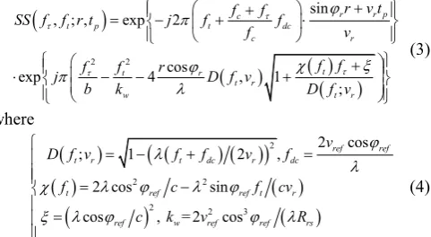
![Fig. 4. Contour plots of the impulse response function from P1 , P5 , and P9 using (a)-(c) the algorithm in [5] (d)-(f) the proposed algorithm](https://thumb-us.123doks.com/thumbv2/123dok_us/7822107.173643/5.595.294.554.307.630/contour-plots-impulse-response-function-algorithm-proposed-algorithm.webp)

