Algorithms for nucleic acid sequence design

(1)

Algorithms for Nucleic Acid Sequence Design

Thesis by

Joseph N. Zadeh

In Partial Fulfillment of the Requirements

for the Degree of

Doctor of Philosophy

California Institute of Technology

Pasadena, California

2010

(2)

Joseph N. Zadeh

(3)

Acknowledgements

First and foremost, I thank Professor Niles Pierce for his mentorship and dedication to this work. He always

goes to great lengths to make time for each member of his research group and ensures we have the best

resources available. Professor Pierce has fostered a creative environment of learning, discussion, and curiosity

with a particular emphasis on quality. I am grateful for the tremendously positive influence he has had on my

life.

I am fortunate to have had access to Professor Erik Winfree and his group. They have been very helpful

in pushing the limits of our software and providing fun test cases. I am also honored to have two other

distinguished researchers on my thesis committee: Stephen Mayo and Paul Rothemund.

All of the work presented in this thesis is the result of collaboration with extremely talented individuals.

Brian Wolfe and I codeveloped the multiobjective design algorithm (Chapter 3). Brian has also been

instru-mental in finessing details of the single-complex algorithm (Chapter 2) and contributing to the parallelization

of NUPACK’s core routines. I would also like to thank Conrad Steenberg, the NUPACK software engineer

(Chapter 4), who has significantly improved the performance of the site and developed robust secondary

structure drawing code. Another codeveloper on NUPACK, Justin Bois, has been a good friend, mentor, and

reliable coding partner. Besides creating many of NUPACK’s back-end compute programs and graphics, he

is also responsible for developing the analysis algorithms with Robert Dirks. Robert, who is also a formidable

speed-chess opponent, laid the groundwork for NUPACK’s compute engine.

I would like to thank Marshall Pierce for helping launch NUPACK. I also owe much gratitude to Asif

Khan, who was instrumental in parallelizing NUPACK, and Miles O’Connell, who provided helpful front-end

programming support. Our talented system administrators also deserve special mention: Chad Schmutzer,

Will Yardley, and Naveed Near-Ansari who have constantly honored our endless lists of esoteric requests.

All of the members of the Pierce Lab have been especially helpful in beta testing NUPACK and providing

useful feedback and discussion. I would also like to recognize Melinda Kirk, who helps keep the lab running

extremely smoothly.

Special thanks are in order to my friends who have provided support and endless laughs along the way:

Elijah Sansom, Neil King, Kevin McHale, Steven Rozenski, Graham Ruby, Victor Beck, Joseph Schramm,

Jane Khudyakov, Jonathan Sternberg, Suvir Venkataraman, Harry Choi, Jennifer Padilla, the Jones family,

(4)

I would especially like to thank my entire family. My aunts Lisa and Faye Majlessi are always

encour-aging. My sister Neda Zadeh, and my brother-in-law Jason Knudson, have provided an endless amount of

moral support. My extremely dedicated and loving parents have cheered me on every step of the way. My

mother, Touran, is always an inspirational figure to me. My father, Khalil, taught me how to program when I

was eight years old, for which I am eternally grateful.

My wonderfully supportive girlfriend, Becca Jones, is a creative inspiration and a bright source of energy

in my life. Her sense of humor makes each day an adventure.

Finally, I would like to dedicate this thesis to my grandfather, the late Mehdi Majlessipour, in memory of

(5)

Abstract

Motivated by a growing field of research focused on programming function into biomolecules, we seek to

de-crease the cost of high-quality rational nucleic acid sequence design while increasing its versatility and

avail-ability. We begin by describing an algorithm for designing the sequence of one or more interacting nucleic

acid strands intended to adopt a target secondary structure at equilibrium. Using ensemble defect

optimiza-tion, we seek to minimize the average number of incorrectly paired nucleotides at equilibrium, calculated over

the entire ensemble of unpseudoknotted secondary structures. Empirically, the algorithm exhibits asymptotic

optimality and costs 4/3 the time of a single objective function evaluation for large structures. We then extend

this algorithm to design multi-state systems with an arbitrary number of linked targets and demonstrate its

efficacy on systems invented by molecular engineers. To improve the ease of use and availability of nucleic

acid analysis and design tools, we present NUPACK, a web application already in wide use that allows the

international research community to share a high-performance compute cluster for the analysis and design of

(6)

List of Figures

1.1 Secondary structure model and loop classification for a single nucleic acid strand . . . 3

2.1 Comparison of test set structural features . . . 13

2.2 Algorithm performance and asymptotic optimality . . . 15

2.3 Computational cost of a single ensemble defect evaluation. . . 16

2.4 Leaf independence and emergent defects . . . 16

2.5 Contributions of hierarchical structure decomposition and defect-weighted sampling to algo-rithm performance. . . 18

2.6 Effect of sequence initialization on algorithm performance. . . 19

2.7 Effect of stop condition stringency on algorithm performance . . . 20

2.8 Algorithm performance on single-stranded and multi-stranded target structures . . . 21

2.9 Effect of design material on algorithm performance . . . 22

2.10 Effect of pattern prevention on algorithm performance . . . 23

2.11 Parallel algorithm performance. . . 24

2.12 Comparison to algorithms inspired by previous publications for the engineered test set . . . . 25

2.13 Comparison to algorithms inspired by previous publications for the random test set . . . 26

3.1 Example of multiobjective decomposition trees . . . 33

3.2 Code for programmable in situ amplification . . . 35

3.3 Multiobjective algorithm run on engineered single-complex input . . . 37

3.4 Multiobjective algorithm run on random single-complex input . . . 38

3.5 Multiobjective performance on systems specified by molecular engineers . . . 39

3.6 Multiobjective design results for a programmable in situ amplification system . . . 40

4.1 Organizational structure of NUPACK . . . 44

4.2 NUPACK navigation bar . . . 45

4.3 NUPACK help popups . . . 45

4.4 Using the NUPACK secondary structure drawing editor to fix overlapping structures . . . 46

4.5 NUPACK secondary structure drawing variations . . . 47

(10)

4.7 NUPACK design input page for single-complex design . . . 52

4.8 NUPACK design execution graph . . . 53

4.9 NUPACK design progress page . . . 54

4.10 NUPACK single-complex design results page . . . 55

4.11 NUPACK single-complex design results detail page . . . 56

4.12 NUPACK multiobjective design input page . . . 57

4.13 NUPACK multiobjective design results page . . . 58

4.14 NUPACK design results detail page for multiobjective design . . . 59

B.1 Structural features of the engineered and random test sets . . . 73

B.2 Code for hybridization chain reaction . . . 74

B.3 Code for synthetic molecular motor . . . 75

B.4 Code forAndlogic gate . . . 75

B.5 Code forOrlogic gate . . . 76

B.6 Code for logic gate single displacement reaction . . . 76

B.7 Code for pair displacement reaction . . . 77

B.8 Code for test tube Dicer system . . . 78

D.1 Example of secondary structure drawing for HU+ notation . . . 84

E.1 NUPACK visits trend . . . 85

(11)

List of Tables

2.1 Default parameter values used in evaluating algorithm performance for RNA design. . . 13

A.1 CPU details . . . 69

(12)

List of Algorithms

2.1 Pseudocode for hierarchical ensemble defect optimization with defect-weighted sampling. . . 12

3.1 Pseudocode for multiobjective, hierarchical ensemble optimization with weighted mutation sampling. . . 36

C.1 Single-scale ensemble defect optimization with uniform mutation sampling. . . 79

C.2 Single-scale ensemble defect optimization with defect-weighted mutation sampling. . . 80

C.3 Hierarchical ensemble defect optimization with uniform sampling. . . 81

C.4 Single-scale probability defect optimization with uniform mutation sampling. . . 82

(13)

Chapter 1

Introduction

Nucleic acids are essential to the survival and proliferation of every living organism. In addition to encoding

genetic information, they have roles in regulation, catalysis, and synthesis [1]. Nucleic acids are also an

attractive nanoscale construction material: besides being intrinsically biocompatible, their synthesis can be

automated [2] and they can be manipulated by a large repertoire of molecular biology techniques developed

over the past half century.

Nucleic acids are linear polymers whose structural unit, the nucleotide, consists of a negatively charged

phosphate group, a sugar, and one of fourbases. Each base is capable of pairing with other bases to form abase pair. This base-pairing mechanism gives nucleic acids a programmablequality and serves as the foundation for the growing field of nucleic acid nanotechnology.

By exploiting pairing specificity, one can rationally design sequences of strands such that hybridization

energies will drive programmed self-assembly of prescribed molecular structures [3]. This has produced a

wide array of engineered nucleic acid systems [4–7] including self-assembling two- and three-dimensional

structures, triggered self-assembly mechanisms, computational devices, machines, scaffolds, and catalysts.

Despite the different approaches and applications of all these nucleic acid systems, they have an important

commonality: they all require the selection of specific sequences that encode the desired structure and

func-tion into the system. We refer to this selecfunc-tion process assequence design.

This thesis focuses on algorithms that encode equilibrium secondary structure into nucleic acid primary

sequences. Our goals are to achieve high-quality, low cost sequence design for both single structures (possibly

multi-stranded) and systems of multiple linked structures. In order to improve the ease of use and accessibility

of these algorithms, we aim to develop a web application for both the design and analysis of nucleic acid

(14)

1.1

Thermodynamic analysis of interacting nucleic acids

1.1.1

Secondary structure model

For an RNA strand withN nucleotides, thesequence,φ, is specified by base identitiesφi ∈ {A,C,G,U}for

i= 1, . . . , N (TreplacesUfor DNA). Thesecondary structureof one or more interacting RNA strands [8] is defined by a set of base pairs (each a Watson Crick pair [A−Uor C−G] or wobble pair [G−U]). By

convention,i·jdenotes that baseiis paired to basej. Strands have directionality (the beginning of the strand

denoted by50and the end by30), with base-pairing occurring in an antiparallel fashion (e.g.,50−GCUCA−30

is fully complementary to50−UGAGC−30).

Apolymer graphfor a secondary structure is constructed byorderingthe strands around a circle, drawing the backbones in succession from 50 to 30 around the circumference with anickbetween each strand, and drawing straight lines connecting paired bases. A secondary structure ispseudoknottedif every strand order-ing corresponds to a polymer graph with crossorder-ing lines. A secondary structure isconnectedif no subset of the strands is free of the others. Anordered complexcorresponds to the unpseudoknotted structural ensemble,Γ, comprising all connected polymer graphs with no crossing lines for a particular ordering of a set of strands.1

For a secondary structure,s∈Γ, thefree energy,

∆G(φ, s) = (L−1)Gassoc+ X

loop∈s

∆G(φ,loop),

is calculated using nearest-neighbor empirical parameters for RNA in 1M Na+ [9, 10] or for DNA in

user-specified Na+ and Mg++ concentrations [11–13], of all loops in that structure. Here, L is the number

of strands in the complex, Gassoc _{is the penalty for strand association [14], and secondary structure loop}

classification is depicted in Figure 1.1. This physical model provides the basis for rigorous analysis and

design of equilibrium base-pairing in the context of the free energy landscape defined over ensembleΓ.

1.1.2

Characterizing equilibrium secondary structure

By calculating thepartition function[17],

Q(φ) =X s∈Γ

e−∆G(φ,s)/kBT_,

overΓ, it is possible to evaluate the equilibrium probability,

p(φ, s) = 1

Q(φ)e

−∆G(φ,s)/kBT_,

(15)

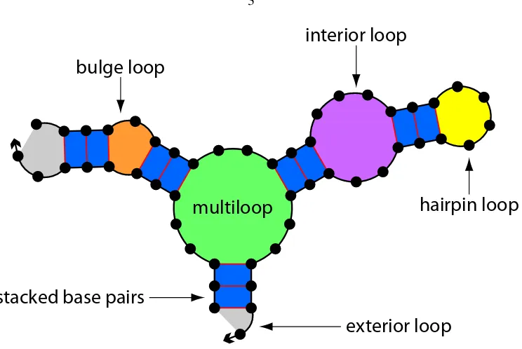
hairpin loop

interior loop

bulge loop

stacked base pairs

[image:15.612.145.517.59.308.2]

exterior loop

multiloop

Figure 1.1: Secondary structure model and loop classification for a single nucleic acid strand. The backbone is represented by the thick directed line with an arrow marking the30end of the strand. Bases are depicted as dots with red lines representing complementary base-pairing. The colors and annotations are used to illustrate the canonical loops [15, 16].

of any secondary structures∈Γ. Here,kBis the Boltzmann constant andT is temperature. The secondary

structure with the highest probability at equilibrium is theminimum free energy(MFE) structure,2satisfying

sMFE(φ) = arg min

s∈Γ∆G(φ, s).

The equilibrium structural features of ensembleΓare quantified by thebase-pairing probability matrix,P(φ), with entriesPi,j(φ)∈[0,1]corresponding to the probability,

Pi,j(φ) =

X

s∈Γ

p(φ, s)Si,j(s), (1.1)

that base pairi·jforms at equilibrium. Here,S(s)is astructure matrixwith entriesSi,j(s)∈ {0,1}. If structurescontains pairi·j, thenSi,j(s) = 1, otherwiseSi,j(s) = 0. For convenience, the structure and

probability matrices are augmented with an extra column to describe unpaired bases. The entrySi,N+1(s) is unity if baseiis unpaired in structure sand zero otherwise; the entry Pi,N+1(φ) ∈ [0,1]denotes the equilibrium probability that baseiis unpaired over ensembleΓ. Hence the row sums of the augmentedS(s)

andP(φ)matrices are unity.

The distance between two secondary structures,s1ands2, is the number of nucleotides paired differently

2_{For simplicity of exposition, we assume that there is a unique MFE structure; only superficial changes are required if this is not the}

(16)

in the two structures:

d(s1, s2) =N− X

1≤i≤N

1≤j≤N+1

Si,j(s1)Si,j(s2).

We also define the discrete delta function

δs1,s2 =

 



1, ifd(s1, s2) = 0,

0, otherwise,

with respect to secondary structure.

Although the size of the ensemble,Γ, grows exponentially with the number of nucleotidesN [18], the MFE structure, the partition function, and the equilibrium base-pairing probabilities can all be calculated via

Θ(N3₎_{dynamic programs [8, 18–25].These dynamic programming algorithms can also be parallelized with} their efficiency to run on multiple computational cores [20, 26].

1.2

Thermodynamic sequence design

For a given target structure,s, we formulate sequence design as an optimization problem, minimizing an

objective function with respect to sequence,φ. Rather than seeking a global optimum, we terminate

opti-mization if the objective function is reduced below a prescribedstop condition.

1.2.1

Objective functions

MFE defect optimization

One strategy is to minimize theMFE defect[20, 27–30]:

µ(φ, s) = d(sMFE, s)

= N− X

1≤i≤N

1≤j≤N+1

Si,j(sMFE(φ))Si,j(s),

(17)

Probability defect optimization

To address this concern, an alternative strategy is to minimize theprobability defect[20, 31, 32]:

π(φ, s) = 1−p(φ, s),

corresponding to the sum of the probabilities of all non-target structures in the ensembleΓ. If π(φ, s) ≈

0, the sequence design is essentially ideal because the equilibrium structural properties of the ensemble are dominated by the target structure s. However, as π(φ, s)deviates from zero, it increasingly fails to characterize the quality of the sequence because the probability defect treats all non-target structures as being

equally defective. This property is a concern for challenging designs where it may be infeasible to achieve

π(φ, s)≈0.

Ensemble defect optimization

To address these shortcomings, a third strategy minimizes theensemble defect[31]:

n(φ, s) = X σ∈Γ

p(φ, σ)d(σ, s) (1.2)

= N− X

1≤i≤N

1≤j≤N+1

Pi,j(φ)Si,j(s), (1.3)

corresponding to the average number of incorrectly paired nucleotides at equilibrium calculated over

ensem-bleΓ.

Comparing formulations

We cast these three objective functions into a unified formulation to highlight their differences:

n(φ, s) = X σ∈Γ

p(φ, σ)d(σ, s),

µ(φ, s) = X σ∈Γ

δσ,sMFEd(σ, s),

π(φ, s) = X σ∈Γ

p(φ, σ)(1−δσ,s).

(18)

discrete delta functionδσ,sMFE, which is unity forsMFEand zero for all other structuresσ∈Γ. Alternatively,

usingπ(φ, s)to perform probability defect optimization,d(σ, s)is replaced by the binary distance function

(1−δσ,s)that is zero forsand 1 for all other structuresσ∈Γ. Hence, the MFE defect makes the optimistic assumption thatsMFE _{will dominate}_Γ _{at equilibrium, while the probability defect makes the pessimistic} assumption that all structuresσ ∈ Γwithd(σ, s) 6= 0are equally distant from the target structures. The objective functionn(φ, s)quantifies the equilibrium structural defects of sequenceφeven whenµ(φ, s)and π(φ, s)do not.

1.2.2

Prior optimization algorithms

The computational challenge of rational sequence design stems from sequence space growing exponentially

with the linear size of the desired target structure. One approach is to employ a local search strategy inspired

by biological evolution to optimize a thermodynamic objective function. These randomized algorithms

ex-plore local neighbors by mutating the identity of a base or base pair followed by an objective function

eval-uation. If the mutation lowered the value of the objective function, the mutation is saved, otherwise it is

accepted with a probability less than one [20, 27, 28, 31–34].

Previous implementations of probability defect optimization [20, 31–33] and ensemble optimization [31]

employedsingle-scalemutation procedures in which each candidate mutation was evaluated on the full se-quence usingΘ(N3₎_{dynamic programs to calculate}_Q₍_φ₎_or_P₍_φ₎_{, respectively. By comparison, more} effi-cienthierarchicalmutation procedures have been developed for MFE defect optimization [20, 27, 28]. These methods perform a hierarchical decomposition of the target structure, optimizing subsequences on a series

of growing substructures to reduce the number of times thatsMFE₍_φ₎_{is calculated on the full sequence using}

aΘ(N3)dynamic program. Furthermore, to reduce the total number of mutations that must be evaluated, these methods guide the selection of candidate mutation positions based on defects in the MFE substructure

[20, 27, 28].

1.3

Thesis outline

Here, we develop an ensemble defect optimization algorithm that employs hierarchical decomposition and

weighted mutation sampling to simultaneously achieve high design quality and low design cost. We then

expand this algorithm to achieve high-quality, low cost ensemble defect optimization for linked multi-state

nucleic acid systems, thus increasing the versatility of nucleic acid design. In order to improve the

accessibil-ity and ease of use of these algorithms, we describe a web application for the design and analysis of nucleic

acid systems.

In Chapter 2 we describe the single-complex design algorithm and perform computational studies that

characterize the algorithmic ingredients and compare performance to previous design approaches. We also

(19)

Motivated by these results and previous invented multi-state nucleic acid systems, in Chapter 3 we improve

the versatility of this algorithm to achieve high-quality designs of multiple linked targets at a reduced cost.

Finally, in Chapter 4, we describe the NUPACK web server for the analysis and design of nucleic acid

(20)

Chapter 2

Nucleic acid sequence design via efficient

ensemble defect optimization

The work in this chapter is based on the following submitted manuscript: J. N. Zadeh, B. R. Wolfe, and N.

A. Pierce. Nucleic acid sequence design via efficient ensemble defect optimization.

2.1

Introduction

Here, we describe a sequence design algorithm that achieves high design quality via ensemble defect

opti-mization, and low design cost via hierarchical structure decomposition and defect-weighted sampling. For

a given target secondary structure,s, withN nucleotides, we seek to design a sequence,φ, with ensemble

defect,n(φ, s), satisfying the stop condition:

n(φ, s)≤fstopN,

for a user-specified value offstop ∈(0,1). Candidate mutations are evaluated at the leaves of a binary tree decomposition of the target structure. During leaf optimization, defect-weighted mutation sampling is used

to select each candidate mutation position with probability proportional to its contribution to the ensemble

defect of the leaf. If emergent structural defects are encountered when merging subsequences moving up the

tree, they are eliminated via defect-weighted child sampling and reoptimization. This design algorithm is

outlined below and detailed in the pseudocode of Algorithm 2.1.

2.2

Algorithm description

2.2.1

Hierarchical structure decomposition

Prior to sequence design, the target structure sis decomposed into a (possibly unbalanced) binary tree of

(21)

child node,kl, and a right child node,kr. Each nucleotide in parent structuresk is partitioned to either the

left or right child substructure (sk ₌_sk l ∪s

k

randskl ∩s k

r =∅). Child nodeklinherits from parent nodekthe

augmented substructure,sk

l+, comprisingnativenucleotides,s

kl

native≡skl, and additionaldummynucleotides

that approximate the influence of its sibling in the context of their parent (skl_≡_skl

native∪s

kl

dummy≡s

k l+). In contrast to earlier hierarchical methods that decompose parent structures at multiloops [20, 27], our

algorithm decomposes parent structures within duplex stems. This approach is more generally applicable

to the design of duplex-rich engineered structures that often contain no multiloops. Eligible split-points are

those locations within a duplex stem with at leastHsplitconsecutive base-pairs to either side, such that both

children would have at leastNsplitnucleotides. If there are no eligible split-points, a structure becomes a leaf

node in the decomposition tree. Otherwise, an eligible split-point is selected so as to minimize the difference

in the size of the children,||sk l| − |s

k

r||. Dummy nucleotides are defined by extending the newly-split duplex

stem across the split-point byHsplitbase pairs (|skdummyl |= 2Hsplit).

For a parent nodek, the sequenceφk _{follows the same partitioning as the structure}_sk ₍_φk ₌_φk l ∪φkr

andφk

l ∩φkr =∅). Likewise, for a child nodekl, the sequence contains both native and dummy nucleotides

(φkl_≡_φkl

native∪φ

kl

dummy≡φ

k l+).

For any nodek with sequenceφk and structuresk, the ensemble defect, nk ≡ n(φk, sk), may be ex-pressed as

nk =X

1≤i≤|sk_| nki,

where

nki = 1−

X

1≤j≤|sk_|₊₁ Pi,jk Si,jk .

is the contribution of nucleotideito the ensemble defect of the node. For a parent nodek, the ensemble defect

can be expressed as a sum of contributions from bases partitioned to the left and right children (nk ₌_nk l+nkr).

For a child nodekl, the ensemble defect can be expressed as a sum of contributions from native and dummy

nucleotides (nkl₌_nkl

native+n

kl

dummy). Conceptually,n

kl

native, the contribution of the native nucleotides to the

ensemble defect of childkl(calculated on child nodeklat costΘ(|skl|3), approximatesnkl, the contribution

of the left-child nucleotides to the ensemble defect of parentk(calculated on parent nodekat higher cost

Θ(|sk_|3₎_{). In general,}_nkl

native 6=n

k

l, because the dummy nucleotides in child nodeklonly approximate the

influence of its sibling (which is fully accounted for only in the more expensive calculation on parent node

k).

The utility of hierarchical structure decomposition hinges on the assumption that sequence space is

suf-ficiently rich that two subsequences optimized for sibling substructures will often not exhibit crosstalk when

merged by a parent node. Our hierarchical mutation procedure is designed to benefit from this property when

(22)

2.2.2

Leaf optimization with weighted mutation sampling

The sequence design process is initializedby randomly specifying the identities of all nucleotides in the leaf structures, subject to the constraint that bases intended to be paired are chosen to be Watson-Crick

complements. At leaf nodek, sequence optimization is performed by mutating either one base at a time (if

Sk

i,|sk_|₊₁ = 1) or one base pair at a time (ifSi,jk = 1for some1≤ j ≤ |sk|, in which caseφki andφkj are

mutated simultaneously so as to remain Watson-Crick complements).

We performdefect-weighted mutation samplingby selecting nucleotideias a candidate for mutation with probabilitynk_i/nk. A candidate sequenceφˆkis evaluated via calculation ofnˆkif the candidate mutation,ξ, is not in the set of previously rejected mutations,γunfavorable(position and sequence). A candidate mutation is

retained ifnˆk _{< n}k_{and rejected otherwise. The set,}_γ_{unfavorable, is updated after each unsuccessful mutation}

and cleared after each successful mutation.

Optimization of leafkterminates successfully if theleaf stop condition:

nk≤fstop|sk|

is satisfied, or restarts ifMunfavorable|sk|consecutive unfavorable candidate mutations are either inγunfavorable or are evaluated and added toγunfavorable. Leaf optimization is attempted from new random initial conditions

up toMleafopttimes before terminating unsuccessfully. The outcome of leaf optimization is the leaf sequence

φkcorresponding to the lowest encountered value of the leaf ensemble defectnk.

2.2.3

Subsequence merging and reoptimization

After sibling nodesklandkrhave been optimized, parent nodekmerges their native subsequences (setting

φk_l =φkl

nativeandφ

k r=φ

kr

native) and evaluatesn

k_{to check the}_{parental stop condition}_:

nk ≤max(fstop|skl|, n kl

native) + max(fstop|skr|, n kr

native).

If this stop condition is satisfied, subsequence merging continues up the tree. Otherwise, failure to satisfy

the stop condition implies the existence ofemergent defectsresulting from crosstalk between the two child sequences. In this case, parent nodekinitiatesdefect-weighted child samplingand reoptimization within its subtree. Left childkl is selected for reoptimization with probabilitynkl/nk and right childkr is selected

for reoptimization with probability nk

r/nk. This defect-weighted child sampling procedure is performed

recursively until a leaf is encountered (each time using partitioned defect information inherited from the

parentkthat initiated the reoptimization). The standard leaf optimization procedure is then performed starting

from a new random initial sequence. The use of random initial conditions during leaf reoptimization is based

on the assumption that sequence space is sufficiently rich that emergent defects can typically be eliminated

(23)

with the reoptimized leaf and its sibling. The elimination of emergent defects in parentkby defect-weighted

child sampling and reoptimization is attempted up toMreopttimes.

2.2.4

Optimality bound and time complexity

This hierarchical sequence design approach implies an asymptotic optimality bound on the cost of designing

the full sequence relative to the cost of evaluating a single candidate mutation on the full sequence. For

a target structure withN nucleotides, evaluation of a candidate sequence requires calculation ofn(φ, s)at costceval(N) = Θ(N3). Performing sequence design using hierarchical structure decomposition, mutations are evaluated at the leaf nodes and merged subsequences are evaluated at all other nodes. For nodek, the

evaluation cost isceval(|sk|). If at least one mutation is required in each leaf, the design cost is minimized by maximizing the depth of the binary tree. Furthermore, at each depth in the tree, the design cost is minimized

by balancing the tree. Hence, a lower bound on the cost of designing the full sequence is given by

cdes(N)≥ceval(N) h

1 + 2 1₂3

+ 4 1₄3

+ 8 1₈3

+. . .i

or

cdes(N)≥

4

3ceval(N).

Hence, if the sequence design algorithm performs optimally for largeN, we would expect the cost of full

sequence design to be 4/3 the cost of evaluating a single mutation on the full sequence. In practice, many

factors might be expected to undermine optimality: imperfect balancing of the tree, the addition of dummy

nucleotides in each non-root node, the use of finite tree depth, leaf optimizations requiring evaluation of

mul-tiple candidate mutations, and reoptimization to eliminate emergent defects. This optimality bound implies

time complexityΩ(N3₎_{for the sequence design algorithm.}

2.3

Methods

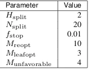
Computational sequence design studies were performed using the default algorithm parameters of Table 2.1.

Design trials were run on a cluster of 2.53 GHz Intel E5540 Xeon dual-processor/quad-core nodes with 24

GB of memory per node.

2.3.1

Structure test sets

Algorithm performance was evaluated on structure test sets containing 30 target structures for each ofN ∈

{100,200,400,800,1600,3200}. Anengineered test set was generated by randomly selecting structural components and dimensions from ranges intended to reflect current practice in engineering nucleic acid

(24)

DESIGNSEQ(φ, s, n, k)

a←DEPTH(k)

ifHASCHILDREN(k)

mreopt←0

ifn=∅

φl←DESIGNSEQ(∅, sl+,∅, kl)

φr←DESIGNSEQ(∅, sr+,∅, kr)

else

UPDATECHILDREN(k, a, a−1)

child, φ←WEIGHTEDCHILDSAMPLING(φ, s, nl, nr)

φchild←DESIGNSEQ(φchild+, schild+, nchild+, kchild)

nk,a_←_E_NSEMBLE_D_EFECT₍_{φ, s}₎ UPDATECHILDREN(k, a, a+ 1)

whilenk,a_>_max(_f

stop|sl|, nkl,anative) + max(fstop|sr|, nkr ,anative)

andmreopt< Mreopt

child,φˆ←WEIGHTEDCHILDSAMPLING(φ, s, nk,a_l , nk,a r )

ˆ

φchild←DESIGNSEQ(φchild+, schild+, nk,achild+, kchild)

ˆ

n←ENSEMBLEDEFECT( ˆφ, s)

ifˆn < nk,a

φ, nk,a←_φ,ˆ_n_ˆ

UPDATECHILDREN(k, a, a+ 1)

mreopt←mreopt+ 1

else

mleafopt←0

φ, nk,a←OPTIMIZELEAF(s)

whilenk,a_{> f}

stop|s|andmleafopt< Mleafopt

ˆ

φ,nˆ←OPTIMIZELEAF(s)

ifˆn < nk,a

φ, nk,a←_φ,ˆ_n_ˆ

mleafopt←mleafopt+ 1

returnφnative UPDATECHILDREN(k, a, b)

ifHASCHILDREN(k)

nkl,a←nkl,b nkr ,a_←_nkr ,b

UPDATECHILDREN(kl, a, b) UPDATECHILDREN(kr, a, b) OPTIMIZELEAF(s)

munfavorable←0

γunfavorable← ∅

φ←INITSEQ(s)

n←ENSEMBLEDEFECT(φ, s)

whilen > fstop|s|andmunfavorable< Munfavorable|s|

ξ,φˆ←WEIGHTEDMUTATIONSAMPLING(φ, s, n1, . . . , n|s|) ifξ∈γunfavorable

munfavorable←munfavorable+ 1

else

ˆ

n←ENSEMBLEDEFECT( ˆφ, s)

ifˆn < n φ, n←_φ,ˆ_n_ˆ

munfavorable←0

γunfavorable← ∅

else

munfavorable←munfavorable+ 1

γunfavorable←γunfavorable

∪

ξ

returnφ, n

(25)

the engineered test set. Each structure in arandomtest set was obtained by calculating an MFE structure of a different random RNA sequence at 37◦C. Figure 2.1 compares the structural features of the engineered and

random test sets. In general, the random test set has target structures with a lower fraction of bases paired,

more duplex stems, and shorter duplex stems (as short as one base pair). Additional structural features of

the engineered and random test sets are summarized in Appendix B, Figure B.1. For the design studies that

follow, new target structure test sets were generated from scratch. The design algorithm was not tested on

these structures prior to generating the depicted results.

Engineered Random

40 Base pairs per stem

0 8 16 24 32

Number of stems 0 2000 3000 c 1000 300 Stems per structure

0 60 120 180 240

Number of structures 0 5 10 15 b Number of structures

0.0 0.2 0.4 0.6 0.8 1.0

0 40 80 120

Fraction of bases paired

[image:25.612.280.368.607.677.2]

a

Figure 2.1: Comparison of the structural features of the engineered and random test sets.

2.3.2

Other algorithms

To illustrate the roles of hierarchical structure decomposition and weighted mutation sampling in the context

of ensemble optimization, we compare our algorithm to three alternative algorithms lacking either or both of

these features:

• Single-scale ensemble defect optimization with uniform mutation sampling[31]. The leaf optimization algorithm is applied directly on the full sequence usinguniform mutation samplingin which each can-didate mutation position is selected with equal probability (pseudocode in Appendix C, Algorithm C.1).

• Single-scale ensemble defect optimization with defect-weighted mutation sampling.The leaf optimiza-tion algorithm is applied directly on the full sequence (pseudocode in Appendix C, Algorithm C.2).

• Hierarchical ensemble defect optimization with uniform mutation sampling.The hierarchical algorithm is applied using uniform mutation sampling during leaf optimization and uniform child sampling during

Parameter Value

Hsplit 2

Nsplit 20

fstop 0.01

Mreopt 10

Mleafopt 3

Munfavorable 4

(26)

subsequence merging and reoptimization (pseudocode in Appendix C, Algorithm C.3).

We also modified our algorithm to compare performance to algorithms inspired by previous work:

• Single-scale probability defect optimization with uniform mutation sampling[20, 31–33]. This method seeks to design a sequence such that the probability defect satisfies the stop conditionπ(φ, s)≤fstop. Satisfaction of this stop condition is sufficient to ensure that stop conditions n(φ, s) ≤ fstopN and µ(φ, s)≤fstopN are also satisfied forfstop ∈ (0,0.5]. Optimization is performed using a modified version of the leaf optimization algorithm (withπ(φ, s)taking the role ofn(φ, s)) applied directly on the full sequence using uniform mutation sampling (pseudocode in Appendix C, Algorithm C.4).

• Hierarchical MFE defect optimization with weighted mutation sampling [20, 27, 28]. This method seeks to design a sequence such that the MFE defect satisfies the stop conditionµ(φ, s) ≤ fstopN. Optimization is performed using a modified version of our algorithm withµk _{taking the role of}_nk

(pseudocode in Appendix C Algorithm C.5).

2.3.3

Implementation

The sequence design algorithm is coded in the C programming language. By parallelizing the dynamic

program for evaluatingP(φ)using MPI [26], the sequence design algorithm can also reduce run time using multiple cores. For a design job allocatedM computational cores, each evaluation ofPk _{for node}_k_with

structuresk_{is performed using}_m_{cores for some}_m_∈₁_{, ..., M}_{selected to approximately minimize run time}

based on|sk_|_{[35]). More implementation and infrastructure details are given in Appendix A.}

2.4

Computational design studies

Our primary test scenario is RNA sequence design at 37◦C for target structures in the engineered test set.

For each target structure in a test set, 10 independent design trials were performed. Each plotted data point

represents a median over 300 design trials (10 trials for each of 30 structures for a given sizeN).

2.4.1

Algorithm performance and asymptotic optimality

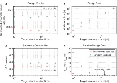
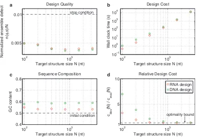
Figure 2.2 demonstrates the typical performance of our algorithm across a range of values ofN using the

engineered and random test sets. Typical designs surpass the desired design quality (n(φ, s)≤N/100) as a result of overshooting stop conditions lower in the decomposition tree (panel a). For the engineered test set,

typical design cost ranges from a fraction of a second forN = 100to roughly three hours forN = 3200

(panel b). For smallN, the design cost for the random test set is higher than for the engineered test set,

becoming comparable asN increases. Typical GCcontent is less than 60% (starting from random initial

(27)

102 103 0.005

0.01

Design Quality

Target structure size N (nt)

Normalized ensemble defect

n(

φ

,s)/N

stop condition

102 103

10−1 100 101 102 103 104 Design Cost

Wall clock time (s)

102 103

0.4 0.5 0.6 0.7 0.8

GC content

Sequence Composition

initial condition

102 103

1 5 10 15 20 25 30 c des (N)

/ c eval

(N)

Target structure size N (nt) Relative Design Cost

Engineered test set Random test set

optimality bound

a b

[image:27.612.132.518.66.340.2]

d c

Figure 2.2: Algorithm performance and asymptotic optimality. a) Design quality. The stop condition is depicted as a dashed line. b) Design cost. c) Sequence composition. The initialGCcontent is depicted as a dashed line. d) Cost of sequence design relative to a single evaluation of the objective function. The optimality bound is depicted as a dashed line. RNA design at 37◦C on the engineered and random test sets.

withN, the relative cost of design,cdes(N)/ceval(N), decreases asymptotically to the optimal bound of 4/3 (panel d). Hence, for sufficiently largeN, the typical cost of sequence design is only 4/3 the cost of a single

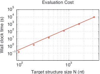
mutation evaluation on the root node. Mutation evaluation has time complexityΘ(N3₎_{and is empirically} observed to be approximately in the asymptotic regime (Figure 2.3). Hence, for our design algorithm, the

empirical observation of asymptotic optimality implies that the exponent in the Ω(N3₎_{time complexity} bound is sharp.

2.4.2

Leaf independence and emergent defects

Figure 2.4 compares the ensemble defect evaluated at the root node, to the sum of the ensemble defects

evaluated at the leaf nodes.1 _{If the assumption of leaf independence is valid (i.e., if dummy nucleotides do a}

good job of mimicking parental environments and there is minimal crosstalk between merged subsequences),

we would expect the data to fall near the diagonal.

For the engineered test set (panel a), we observe three striking properties. First, for random initial

se-quences, the assumption of leaf independence is well-justified despite the fact that the ensemble defect is

large. Second, leaf optimization followed by merging without reoptimization (i.e.,Mreopt = 0) typically 1_{To avoid overcounting defects at the leaves,}_nk

(28)

102 103 10−1

100 101 102 103 104 105

Wall clock time (s)

[image:28.612.240.410.105.231.2]

Target structure size N (nt) Evaluation Cost

Figure 2.3: Computational cost,ceval(N) = Θ(N3), of a single evaluation of the ensemble defect,n(φ, s), for the full sequence and target structure. Each data point represents the median over all sequences for a particular value ofN. The line depicts a slope of three, suggesting empirically that the dynamic program is operating approximately within the asymptotic regime for this range ofN. RNA design at 37◦C on the engineered test set.

10−3 10−2 10−1 100

[Sum of leaf n(φ,s)]/N

Root n(

φ

,s)/N

Random sequences Leaf−optimized sequences Final sequence designs

10−3 10−2 10−1 100

[Sum of leaf n(φ,s)]/N

Root n(

φ

,s)/N

a b

[image:28.612.133.516.387.617.2]

(29)

yields full sequence designs that achieve the desired design quality (n(φ, s) ≤ N/100on the root), with emergent defects arising only in a minority of cases. Third, these emergent defects are successfully

elimi-nated by defect-weighted child sampling and reoptimization starting from new random initial subsequences.

The resulting full sequence designs exhibit leaf independence and satisfy the stop condition.

By comparison, for the random test set, merging of leaf-optimized sequences typically does lead to

emer-gent defects in the root node. Even in this case, our algorithm successfully eliminates emeremer-gent defects using

defect-weighted child sampling and reoptimization starting from new random initial subsequences.

2.4.3

Contributions of algorithmic ingredients

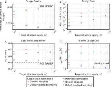
Figure 2.5 isolates the contributions of hierarchical structure decomposition and defect-weighted sampling to

our ensemble defect optimization algorithm by comparing performance to three modified algorithms lacking

one or both ingredients. All four methods typically achieve the desired design quality, with hierarchical

methods surpassing the quality requirement for the root node as a result of overshooting stop conditions

lower in the decomposition tree. Hierarchical methods dramatically reduce design cost relative to their

single-scale counterparts (which are not tested forN = 800due to high cost). Defect-weighted sampling reduces design cost andGCcontent by focusing mutation effort on the most defective subsequences. For the

single-scale methods, the relative cost of design,cdes(N)/ceval(N), increases withN. For hierarchical methods, cdes(N)/ceval(N)decreases asymptotically to the optimal bound of 4/3 asN increases. Our algorithm thus combines the design quality of ensemble defect optimization, the reduced cost and asymptotic optimality of

hierarchical decomposition, and the reduced cost and reducedGCcontent of defect-weighted sampling.

2.4.4

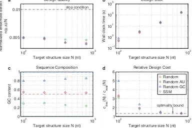
Sequence initialization

To explore the effect of sequence initialization on typical design quality and cost, we tested four types of initial

conditions (Figure 2.6): random sequences (default), random sequences using onlyAandTbases, random

sequences using onlyGandCbases, and sequences satisfying sequence symmetry minimization (SSM) [3].2

The desired design quality is achieved independent of the initial conditions (panel a), which have little effect

on design cost (panels b and d). Designs initiated with randomATsequences or with randomGCsequences

illustrate that the ensemble defect stop condition can be satisfied over a broad range ofGCcontents (panel c).

2.4.5

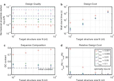
Stop condition stringency

Figure 2.7 depicts typical algorithm performance for five different levels of stringency in the stop condition:

fstop ∈ {0.001,0.005,0.01(default),0.05,0.10}. For each stop condition, the observed design quality is better than required (resulting from overshooting stop conditions lower in the decomposition tree). Consistent

2_{SSM is a heuristic that promotes specificity for the target structure by prohibiting repeated subsequences of a specified word length}

(30)

102 103 0.005

0.01

Design Quality

n(

φ

,s)/N

stop condition

102 103

10−1 100 101 102 103 104

105 Design Cost

Wall clock time (s)

102 103

0.4 0.5 0.6 0.7 0.8

GC content

initial condition

102 103

100 101 102 103 c des (N)

/ c eval

(N)

Uniform sampling

Defect-weighted sampling Uniform samplingDefect-weighted sampling

optimality bound

Single-scale optimization Hierarchical optimization

a b

[image:30.612.133.516.203.505.2]

d c

(31)

102 103 0.005

0.01

Design Quality

n(

φ

,s)/N

stop condition

102 103

10−1

100

101

102

103 Design Cost

Wall clock time (s)

102 103

0 0.2 0.4 0.6 0.8 1

GC content

102 103

1 2 3 4 5 6 c des (N)

/ c eval

(N)

[image:31.612.134.518.234.491.2]

Random Random AU Random GC SSM optimality bound a b d c

(32)

102 103 10−4

Design Quality

n(

φ

,s)/N

102 103

10−1 100 101 102

103 Design Cost

Wall clock time (s)

102 103

0.4 0.5 0.6 0.7 0.8

GC content

initial condition

102 103

1 10 20 30 c des (N)

/ c eval

(N)

f_stop = 0.001 f_stop = 0.005 f_stop = 0.01 f_stop = 0.05 f_stop = 0.1

[image:32.612.132.517.64.337.2]

optimality bound 10−3 10−1 10−2 a b d c

Figure 2.7: Effect of stop condition stringency on algorithm performance. a) Design quality. Stop conditions are depicted by dashed lines. b) Design cost. c) Sequence composition. The initialGCcontent is depicted as a dashed line. d) Cost of sequence design relative to a single evaluation of the objective function. The optimality bound is depicted as a dashed line. RNA design at 37◦C on the engineered test set.

with empirical asymptotic optimality, the design cost is independent offstopfor sufficiently largeN (for the

tested stringency levels). It is noteworthy that the algorithm is capable of routinely and efficiently designing

sequences with ensemble defect less thanN/1000.

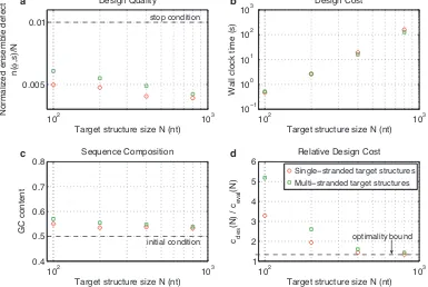
2.4.6

Multi-stranded target structures

Multi-stranded target structures arise frequently in engineering practice [4, 5, 7]. Figure 2.8 demonstrates that

our algorithm performs similarly on single-stranded and multi-stranded target structures.

2.4.7

Design material

Figure 2.9 compares RNA and DNA design. DNA designs are performed in 1 M Na+_{at 23}◦_{C to reflect that}

DNA systems are typically engineered for room temperature studies. In comparison to RNA design, DNA

design leads to similar design quality (panel a), higher design cost (panel b), and somewhat higherGCcontent

(33)

102 103 0.005

0.01

Design Quality

n(

φ

,s)/N

stop condition

102 103

10−1 100 101 102

103 Design Cost

Wall clock time (s)

102 103

0.4 0.5 0.6 0.7 0.8

GC content

initial condition

102 103

1 2 3 4 5 6 c des (N)

/ c eval

(N)

Target structure size N (nt) Relative Design Cost Single−stranded target structures Multi−stranded target structures

optimality bound

a b

[image:33.612.133.518.233.491.2]

d c

(34)

102 103 0.005

0.01

Design Quality

n(

φ

,s)/N

stop condition

102 103

10−1 100 101 102 103 104 Design Cost

Wall clock time (s)

102 103

0.4 0.5 0.6 0.7 0.8

GC content

initial condition

102 103

1 5 10

c des

(N)

/ c eval

(N)

[image:34.612.132.520.223.494.2]

RNA design DNA design optimality bound a b d c

(35)

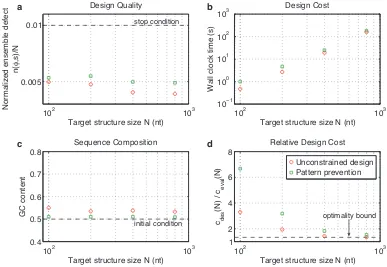
2.4.8

Sequence constraints and pattern prevention

Molecular engineers sometimes constrain the sequence of certain nucleotides in the target structure (e.g., to

ensure complementarity to a specific biological sequence), or prevent certain patterns from appearing

any-where in the design (e.g.,GGGG). Our algorithm accepts sequence constraints and pattern prevention

require-ments expressed using standard nucleic acid codes.3_{Figure 2.10 demonstrates that the prevention of patterns}

{AAAA,CCCC,GGGG,UUUU,KKKKKK,MMMMMM,RRRRRR,SSSSSS,WWWWWW,YYYYYY}has little effect on

de-sign quality orGCcontent (panels a and c), and somewhat increases design cost while retaining asymptotic

optimality (panels b and d).

102 103

0.005 0.01

Design Quality

n(

φ

,s)/N

stop condition

102 103

10−1 100 101 102

103 Design Cost

Wall clock time (s)

102 103

0.4 0.5 0.6 0.7 0.8

GC content

initial condition

102 103

1 2 4 6 8 c des (N)

/ c eval

(N)

[image:35.612.130.517.229.496.2]

Unconstrained design Pattern prevention optimality bound a b d c

Figure 2.10: Effect of pattern prevention on algorithm performance. a) Design quality. The stop condition is depicted as a dashed line. b) Design cost. c) Sequence composition. The initialGCcontent is depicted as a dashed line. d) Cost of sequence design relative to a single evaluation of the objective function. The optimality bound is depicted as a dashed line. RNA design at 37◦C on the engineered test set.

2.4.9

Parallel efficiency and speedup

The contour plots of Figure 2.11 demonstrate the parallel efficiency and speedup achieved using a parallel

implementation of the design algorithm onM computational cores (efficiency(N, M)=t(N,1)/(t(N, M)× M), speedup(N, M)=t(N,1)/t(N, M), wheretis wall clock time). Using two computational cores, the 3_{During leaf optimization, mutation candidates are not considered if they would introduce a pattern violation. Pattern violations that}

(36)

0.0 0.1 0.2 0.3 0.5 0.4 0.6 0.7 0.8 0.9 1.0

Number of computational cores

20 21 22 23 24 25

Target structure size N (nt) 102 103

Number of computational cores

20 21 22 23 24 25

Target structure size N (nt) 102 103 0 2 4 6 8 10 14 12

a Parallel Efficiency b Parallel Speedup

Figure 2.11: Parallel algorithm performance. a) Parallel efficiency and b) parallel speedup using multiple computational cores. Dashed lines denote boundaries between nodes, indicating the use of message passing. RNA design at 37◦C on the engineered test set.

parallel efficiency exceeds≈0.9 for target structures withN > 400. Using 32 computational cores, the parallel speedup is≈14for target structures withN = 3200.

2.4.10

Comparison to previous methods

Figure 2.12 compares the performance of our algorithm to the performance of algorithms inspired by previous

publications. Single-scale methods that employ uniform mutation sampling to optimize either ensemble

de-fect or probability dede-fect achieve the desired design quality at significantly higher cost and with significantly

higherGCcontent (panels a-c). Sequences resulting from probability defect optimization typically surpass

the ensemble defect stop condition despite failing to satisfy the probability defect stop condition (panel e),

reflecting the pessimism ofπ(φ, s)in characterizing the equilibrium structural defect over ensembleΓ. For either single-scale method, the relative cost of design,cdes(N)/ceval(N), increases withN (panel d). Owing to the high cost of the single-scale approaches, designs were not attempted for largeN.

By contrast, hierarchical MFE defect optimization with defect-weighted sampling leads to efficient

satis-faction of the MFE stop condition (panels b and f), exhibiting asymptotic optimality withcdes(N)/ceval(N) approaching 4/3 for largeN (panel d). Asymptotically, the cost of hierarchical MFE optimization relative to

hierarchical ensemble defect optimization is lower by a constant factor corresponding to the relative cost of

evaluating the two objective functions usingΘ(N3)dynamic programs (panels b and d). The shortcoming of MFE defect optimization is the unreliability ofsMFE₍_φ₎_{in characterizing the equilibrium structural properties}

of ensembleΓ[31]. Despite satisfying the MFE defect stop condition, sequences designed via MFE defect optimization typically fail to achieve the ensemble defect stop condition by roughly a factor of five for the

(37)

−2 −1 0 1 2 3 4 5 0 1 2 3 4 5 0.0 0.02 0.04 0.06 0.08 0.1

n( φ ,s)/N 10 10 10 10 10 10 10 10

Wall clock time (s)

0.4 0.5 0.6 0.7 0.8 GC content 10 10 10 10 10 10 des eval c (N) / c (N) 0 0.005 0.010

Normalized MFE defect

μ ( φ ,s)/N 0 0.2 0.4 0.6 0.8 Probability defect π ( φ ,s) a b d c f e ₁

2 3 2 3

10 10

Design Quality

Target structure size N (nt) 10 10

Design Cost

10 10

Target structure size N (nt) Sequence Composition

10 10

0 0.05 0.1

Normalized ensemble defect n(φ,s)/N

0 0.05 0.1

Normalized ensemble defect n(φ,s)/N

optimality bound initial condition

stop condition

[image:37.612.128.517.109.576.2]

Single−scale probability defect optimization Single−scale ensemble defect optimization Hierarchical MFE defect optimization Hierarchical ensemble defect optimization

(38)

102 103 0.00 0.05 0.10 0.15 0.20 0.25

0.30 Design Quality

n(

φ

,s)/N

102 103

10−2 10−1 100 101 102 103 104

105 Design Cost

Wall clock time (s)

102 103

0.4 0.5 0.6 0.7 0.8

GC content

102 103

100 101 102 103 104 105 cdes (N)

/ ceval

(N)

0 0.05 0.1 0.15 0.2 0.25

0.1 0.2 0.3 0.4 0.5

n(φ,s)/N

Normalized MFE defect

μ

(

φ

,s)/N

0 0.05 0.1 0.15 0.2 0.25

0 0.2 0.4 0.6 0.8 1

n(φ,s)/N

Probability defect π ( φ ,s) a b d c f e 0

Single−scale probability defect optimization Single−scale ensemble defect optimization Hierarchical MFE defect optimization Hierarchical ensemble defect optimization stop condition

[image:38.612.129.517.113.571.2]

initial condition optimality bound

(39)

2.5

Discussion

Our algorithm combines four major ingredients to design the sequenceφof one or more strands intended to

adopt target secondary structuresat equilibrium:

• Ensemble defect optimization:The design objective function is the ensemble defect,n(φ, s), represent-ing the average number of incorrectly paired nucleotides at equilibrium calculated over the ensemble of

unpseudoknotted secondary structuresΓ. For a target structure withN nucleotides, we seek to satisfy the stop condition:n(φ, s)≤fstopN.

• Hierarchical structure decomposition:We perform a binary tree decomposition of the target secondary structure, decomposing each parent structure within a duplex stem, and introducing dummy nucleotides

to extend the truncated duplex in each child structure to mimic the parental environment.

• Leaf optimization with defect-weighted mutation sampling:Starting from a random initial sequence, se-quence optimization is performed in the leaf nodes using defect-weighted mutation sampling in which

each candidate mutation position is selected with probability proportional to its contribution to the

ensemble defect of the leaf.

• Subsequence merging and reoptimization: As subsequences are merged moving up the tree, a parent node initiates defect-weighted child sampling and reoptimization within its subtree only if there are

emergent defects resulting from crosstalk between child subsequences. Leaf reoptimization starts from

a new random initial sequence.

Using aΘ(N3)dynamic program to evaluate the design objective function, we derive an asymptotic opti-mality bound on design time: for largeN, the minimum cost to design a sequence withNnucleotides is 4/3

the cost of evaluating the objective function once onN nucleotides. Hence, our design algorithm has time

complexityΩ(N3₎_.

We studied the performance of our algorithm in the context of empirical secondary structure free

en-ergy models [10, 11] that have practical utility for the analysis [36–40] and design [41–46] of functional

nucleic acid systems. In particular, we examined RNA design at 37◦C on target structures containing

N ∈ {100,200,400,800,1600,3200}nucleotides and duplex stems ranging from 1 to 30 base pairs. Empir-ically, we observe several striking properties:

• Emergent defects are sufficiently infrequent that they can typically be eliminated by leaf reoptimization

starting from new random initial sequences.

(40)

• Our algorithm exhibits asymptotic optimality for largeN, with full sequence design costing roughly

4/3 the cost of a single evaluation of the objective function. Hence, the algorithm is efficient in the

sense that the exponent in theΩ(N3₎_{time complexity bound is sharp.}

We modified our algorithm to compare performance to algorithms inspired by previous work [20, 27–29,

31, 32]. In line with conceptual expectations, we observe empirically that our algorithm achieves lower design

cost relative to single-scale probability or ensemble defect optimization with uniform mutation sampling, and

higher design quality relative to hierarchical MFE defect optimization with defect-weighted sampling.

To enhance the utility of our algorithm for molecular engineers, our algorithm addresses several

practi-cal considerations, including: sequence constraints, pattern prevention, multi-stranded target structures, and

(41)

Chapter 3

Sequence design for multi-state nucleic

acid systems

Motivated by the design of multi-state nucleic acid systems [41, 44–47], we wish to extend the quality and

efficiency of the single-complex algorithm to the design of multiple strands that interact conditionally to form

multiple different target structures. Most of these dynamic systems involve pathways of interactions between

complexes. For instance, a disassembly reaction involving one complex might release a strand that engages

in a self-assembly reaction with another complex. For these types of interactions to occur, the identities of

certain bases across the multiple ordered complexes may be linked.

Our early approaches to using ensemble defect optimization for the design of multi-state systems

em-ployed single-scale algorithms. These algorithms successfully designed systems that exhibited the desired

behavior [41, 44, 45], but were costly, as one would expect from our single-scale computational studies

pre-sented in Chapter 2. Here we extend the scope of our single-complex design algorithm to include the design

of multiple ordered complexes with related sequences.

3.1

Objective function

The design of multiple ordered complexes can be formulated as a multiobjective optimization problem,

min-imizing the ensemble defect of each sequence in Φ = {φ1, ..., φR} relative to a set of target structures Ψ ={s1, ..., sR}simultaneously,

n(φt, st)< fstopNt ∀st∈Ψ.

Thus, we wish to achieve the same single-objective stop condition on each ordered complex inΨ. In order to maintain the efficiency and quality, our approach preserves the same algorithmic ingredients from the

(42)

3.2

Sequence linkages

In addition to providing a set of ordered complexes Ψ, the algorithm also requires a set of linkages Ξ =

{η1, ..., ηz} where each linkage η is a quintuplehsa, i, sb, j, ρirepresenting the base-pairing relationship

ρ ∈ {complementary,identical} between the base at positioniin complexsa and the base at positionj

in complexsb. Thus, inΦ, baseiin sequenceφa must be either complementary or identical to basej in

sequenceφb. Furthermore, linkages can exist within the same structure (i.e.,sa = sb) and each base can

participate in multiple linkages.

3.3

Optimality bound and time complexity

Since the multiobjective algorithm is attempting to design multiple decomposition trees simultaneously, the

asymptotic optimality bound is the sum over the bounds of designing those trees independently and is given

by

cdes(Ψ)≥

4 3

X

s∈Ψ

ceval(s).

3.4

Multiobjective ensemble defect optimization algorithm

3.4.1

Synchronizing linkages

The existence of a set of linkagesΞimplies that a mutation at one base could potentially affect multiple other bases elsewhere in the system. To keep bases in sync, the algorithm employs aglobal sequence table, GST, with each entry corresponding to a base identity. The quintuples inΞare used to assign a global index in this table to each base position in each structurest∈ Ψ. Thus, in the quintuplehsa, i, sb, j, ρi, positioniinsa

and positionjinsbwill be assigned the same global index as will all other linked related bases. In addition

to each base being assigned an index in the GST, each base will also be assigned a relationshipρto that entry

in the GST.

Each mutation requires an update to the global sequence table. It also follows that prior to objective

function evaluation, all bases will be synchronized with the the global sequence table.

3.4.2

Multi-state hierarchical decomposition

Each structure inΨis decomposed with the same single-complex technique outlined in Section 2.2.1. The decomposition process also ensures that each base in the decomposition tree also has the appropriate GST

index.

We will refer to the set of all nodes in all decomposition trees as ΨD _{and the leaves as} _ΨL _⊆ _ΨD_.

Individual nodes,sk

(43)

3.4.3

Multi-leaf optimization with weighted mutation sampling

The algorithm makes mutations to nodes inΨL_{with the goal of satisfying the stop condition}

n(φkt, skt)≤fstop|skt| ∀skt ∈ΨL.

To determine which leaves are not satisfied and thus eligible for mutation, we define an ensemble defect

threshold function,

nthreshold(φkt, s k t) =

 



n(φkt, skt) :n(φkt, skt)> fstop|skt| 0 :n(φkt, stk)≤fstop|skt|

,

that is used to weigh which leaf should be optimized next. The probability of a selecting a leafsk∗ t∗ for mutation isnthreshold(φk

∗ t∗, sk

∗ t∗)/P_sk

t∈ΨLnthreshold(φ

k

t, skt). Once a leaf is selected, mutations are weighted

according to the same defect sampling scheme of the single-complex algorithm, described in Section 2.2.2.

After a mutation is made, the other leaves must be synchronized with the GST. To determine if the

mutation brought the multiple objectives closer to the stop condition, we calculaten(φkt, skt)for each leaf

and sum the thresholding functions. The mutation is retained if

X

sk t∈ΨL

nthreshold( ˆφkt, s k t)<

X

sk t∈ΨL

nthreshold(φkt, s k t).

Thus, when

X

sk t∈ΨL

nthreshold(φkt, s k t) = 0,

the stop condition has been reached.

As in single-complex design, we keep a list of previously rejected mutations,γk

t, for each leaf1. Thus, a

mutation that propagates to several other leaves must be retained in each leaf’sγ_tk list. If leafsk_t accepts a mutation, even if that mutation originated elsewhere, it must clear itsγtk list. Likewise, any failed mutation

must be stored locally in each affected leaf’sγtk.

Optimization of leaves terminates successfully if the stop condition is satisfied or unsuccessfully if

Munfavorable|skt| consecutive unfavorable candidate mutations are either inγtk or are evaluated and added

toγk

t for all leavesskt ∈ΨL.

This leaf optimization procedure is reinitialized and reoptimized up to Mleafopt times. With each

at-tempt, leaves that did not satisfy the stop condition are reinitialized. Note that reinitialization may propagate

mutations to leaves that were previously satisfied.

1_{In the single-complex algorithm, we maintained only one}_{γunfavorable}_{since only one leaf was optimized at a time. However, in}

the multiobjective case we must maintain separate listsγk

(44)

3.4.4