ResearchOnline@JCU
This is the author-created version of the following work:
Jarvis, Diane, Stoeckl, Natalie, and Liu, Hong-Bo (2017)
New methods for
valuing, and for identifying spatial variations, in cultural services: a case study of
the Great Barrier Reef.
Ecosystem Services, 24 pp. 58-67.
Access to this file is available from:
https://researchonline.jcu.edu.au/47535/
© 2017. This manuscript version is made available under a Creative Commons
license CC-by-NC-ND (https://creativecommons.org/licenses/by-nc-nd/4.0/).
1 2 3 4 5 6 7 8 9 10 11 12 13 14 15 16 17 18 19 20 21 22 23 24 25 26 27 28 29 30 31 32 33 34 35 36 37 38 39 40 41 42 43 44 45 46 47 48 49 50 51 52 53 54 55 56 57 58 59 60 61
New methods for valuing, and for identifying spatial
variations, in cultural services: A case study of the
Great Barrier Reef
Diane Jarvisa*, Natalie Stoecklb, Hong-Bo Liub
a
James Cook University, P. O. Box 6811, Cairns, Queensland 4870, Australia
b
James Cook University, Townsville, Queensland 4811, Australia
*Corresponding author
Email addresses and phone number of corresponding author:
[email protected] Tel: +61 (7) 423 21371
Title page
1 2 3 4 5 6 7 8 9 10 11 12 13 14 15 16 17 18 19 20 21 22 23 24 25 26 27 28 29 30 31 32 33 34 35 36 37 38 39 40 41 42 43 44 45 46 47 48 49 50 51 52 53 54 55 56 57 58 59 60 61
New methods for valuing, and for identifying spatial
variations, in cultural services: A case study of the
Great Barrier Reef
Abstract
Estimating values for ecosystem services (ES) can contribute to the decision making process, reducing the risk that ES benefits are overlooked. For ES with no (direct or indirect) links to markets, valuation is a non-trivial exercise. Traditional methods require the use of hypothetical markets; the life satisfaction (LS) approach does not. LS has previously been used to estimate the value of regulating ES, but to the best of our knowledge has never been used to estimate the value of Cultural
services (CS).
We examine the relationship between LS and a subset of CS provided by the Great Barrier Reef (GBR), (the non-use CS), using geographically weighted regression to investigate spatial variations in value. After controlling for other factors, we find income is more important to LS in the south than the north; the opposite is true for non-use CS.
The coefficients are used to estimate the amount of income required to keep overall LS constant, should the non-use CS of the GBR not be preserved, estimated at $8.7bn annually. We acknowledge the imperfections of our work, noting the need for research on better CS measures, but feel that the general approach may add another useful tool to the valuation toolbox.
Highlights
Focuses on the value of ecosystem services provided by the Great Barrier Reef (GBR)
Uses life satisfaction (LS) approach to estimate cultural ecosystem services values
Uses geographically weighted regression for spatial analysis
Finds income (cultural services) more important to LS in the south (north)
Estimates the GBR’s cultural ecosystem services value at approx. $8.7 bn per annum
Revised manuscript
1 2 3 4 5 6 7 8 9 10 11 12 13 14 15 16 17 18 19 20 21 22 23 24 25 26 27 28 29 30 31 32 33 34 35 36 37 38 39 40 41 42 43 44 45 46 47 48 49 50 51 52 53 54 55 56 57 58 59 60 61
Keywords
Cultural services; Non-market valuation; Geographically weighted regression; Life satisfaction; Spatial analysis of life satisfaction; Great Barrier Reef.
1
Introduction
Ecosystems provide mankind with an extensive range of goods and services that are critical to human welfare (Costanza et al., 1997; Daily et al., 2000). Valuation of ecosystem services (ES) is a useful tool available to decision makers tasked with managing resources (Daily et al., 2000). Monetising ES can provide a range of benefits that can help inform resource allocation decisions, including highlighting the appropriate weighting of vital services (Costanza et al., 1997), raising awareness about the importance of ES (de Groot et al., 2012), and making explicit the costs of ES degradation (Pascual et al., 2010).
Valuation has been criticised for not only failing to help conserve many of the world’s ES, but by
assisting the commodification process, facilitating their loss or degradation, (Gómez-Baggethun, de Groot, Lomas, & Montes, 2010; Gómez-Baggethun & Ruiz-Pérez, 2011). However, ‘valuing ES is not identical to commodifying them for trade in private markets’ (Costanza, 2006, p. 749), and need not lead to commodification (Gómez-Baggethun & Ruiz-Pérez, 2011). Indeed, the diverse nature of ES suggests that whilst some services may be susceptible to commodification, the complex overlapping and entangled benefits provided by many ES make it difficult to either monetise a single particular ES (Stoeckl, Farr, Larson, et al., 2014) or to separate a single function into a discrete commodifiable unit (Gómez-Baggethun & Ruiz-Pérez, 2011).
Some ES are easier to value than others, with cultural services being particularly difficult. Cultural services (CS) are the “nonmaterial benefits people obtain from ecosystems through spiritual enrichment, cognitive development, reflection, recreation and aesthetic experiences” (Millennium
1 2 3 4 5 6 7 8 9 10 11 12 13 14 15 16 17 18 19 20 21 22 23 24 25 26 27 28 29 30 31 32 33 34 35 36 37 38 39 40 41 42 43 44 45 46 47 48 49 50 51 52 53 54 55 56 57 58 59 60 61
from people’s beliefs or understandings” (Haines-Young & Potschin, 2013, p. 18). CS have been
described as comprising aesthetic information, opportunities for recreation and tourism, inspiration for culture, art and design, spiritual experience, and information for cognitive development (de Groot et al., 2010), or more succinctly, as encompassing cultural heritage, recreation and tourism, and aesthetic values (Pascual et al., 2010). Recreation and tourism aside, many other CS provide the type of benefits that people would assign what economists term non-use values (Krutilla, 1967; Weisbrod, 1964). Thus, CS essentially provide a hybrid of use and non-use benefits, each of which contribute to the overall value (use and non-use) assigned to the CS (Braat & de Groot, 2012; Pascual et al., 2010). A core problem of this being that the values assigned to the non-use CS are not traceable through well-functioning markets, or indeed through any market at all (Costanza et al., 1997).
Omitting non-use values of CS from valuation estimates risks excluding that which people may care about most (Carson, Flores, & Meade, 2001). Traditional non-market valuation approaches that have been explicitly developed to measure non-use values (such as contingent valuation, choice modelling) assume that utility is cardinally unobservable (Gowdy, 2005), requiring researchers to work with indirect utility functions derived from hypothetical markets. However, an emerging body of research has established that measures of life satisfaction (LS) or subjective well-being can serve as a proxy for utility (Kristoffersen, 2010) at both the microeconomic (Ferreira & Moro, 2010), and macroeconomic (Engelbrecht, 2009) level. Simplistically, LS researchers ask questions, such as “how satisfied are you with your life as a whole?”, and responses are then regressed against a variety of other factors, the
1 2 3 4 5 6 7 8 9 10 11 12 13 14 15 16 17 18 19 20 21 22 23 24 25 26 27 28 29 30 31 32 33 34 35 36 37 38 39 40 41 42 43 44 45 46 47 48 49 50 51 52 53 54 55 56 57 58 59 60 61
2014). But to the best of our knowledge, no-one has yet attempted to use the LS approach to assess the value of CS - the focus of this paper.
The LS approach lends itself to the valuation of CS in a number of different ways. The approach is neither rooted in the biophysical nor financial domains which are known to impact the values elicited, failing to fully reflect the social-cultural impact of ES (Martin-Lopez, Gomez-Baggethun, Garcia-Llorente, & Montes, 2014). It clearly focuses on the relationship between the environment and human well-being (as measured by the LS of individuals), which forms the root of the development of the ES concept (Martin-Lopez et al., 2014) and aims at the core objective of much welfare economics, namely to maximise (individual and/or social) welfare (utility). It also may be able to make a useful contribution to situations involving ‘taboo trade-offs’ where morally or culturally it is virtually
impossible for an individual to contemplate a financial value for something considered sacred, such as a human life (Daw et al., 2015)1.
The LS approach assumes that each explanatory factor enters the function in a separable and additive manner, but there is much potential overlap between factors (Stoeckl, Farr, Larson, et al., 2014; Windle & Rolfe, 2005); the implication is that this needs to be tested for before simply entering each factor as a separate contributor to LS. Location specific factors (e.g. scenic views, pollution, climate) also impact people’s subjective satisfaction with those factors and/or the importance people assign to
those factors as contributors to LS (Costanza et al., 2007). An implication of these location specific factors is that the relationship between CS and LS may vary across geographic regions. Estimating a single (regression) equation for all individuals across a wide geographic region implicitly assumes that all factors contribute similarly to the LS of all individuals in all locations; thus if regional variations are present global estimation techniques will not model relationships well and alternate techniques that address spatial relationships, such as geographically weighted regression (GWR), may be required to avoid biased or invalid estimation results (Bateman, Jones, Lovett, Lake, & Day, 2002).
1
1 2 3 4 5 6 7 8 9 10 11 12 13 14 15 16 17 18 19 20 21 22 23 24 25 26 27 28 29 30 31 32 33 34 35 36 37 38 39 40 41 42 43 44 45 46 47 48 49 50 51 52 53 54 55 56 57 58 59 60 61
This paper takes a LS approach to demonstrate a way of assessing the value of CS, whilst also employing an estimation technique that can account for potential spatial variations in the relationship between LS and CS (not previously used in LS valuation studies). Here, we use the Great Barrier Reef World Heritage Area (GBR) as a case study to ask:
1. Do reported levels of satisfaction with the CS associated with the GBR contribute to the overall satisfaction with life reported by residents, and is there spatial variation within this relationship? 2. Can we use coefficients from the LS model to generate valid estimates of (some of) the CS values
of the GBR?
Within section 2 we briefly describe our case study area, the development of our model, the selection of our independent variables, and the design of our questionnaire. We also describe how the data were collected, our estimation techniques, and our method of estimating the value of CS. Results are provided and discussed in section 3, whilst section 4 draws conclusions from this research.
2
Materials and methods
2.1
Case study area
The GBR, situated in the Coral Sea off the coast of Queensland, Australia, is the world’s largest reef
1 2 3 4 5 6 7 8 9 10 11 12 13 14 15 16 17 18 19 20 21 22 23 24 25 26 27 28 29 30 31 32 33 34 35 36 37 38 39 40 41 42 43 44 45 46 47 48 49 50 51 52 53 54 55 56 57 58 59 60 61
Numerous studies in recent decades have generated estimates of the monetary worth of various values associated with the GBR, although there have been many more studies of the services provided via markets (predominantly use values) where values are relatively easy to estimate (Stoeckl et al., 2011). Studies of non-use values are relatively sparse but include: a contingent valuation study of ‘vicarious’ users (tourists and Australian residents living outside the GBR catchment) (Hundloe, Vanclay, & Carter, 1987); a choice modelling study of the non-use value of an estuary within the GBR catchment (Windle & Rolfe, 2005); and an attempt to estimate the collective value of numerous community defined benefits, grouped together to represent either provisioning services, regulation and maintenance services, cultural services, or a mix of cultural and regulation and maintenance service (Stoeckl, Farr, Larson, et al., 2014). Thus, the existing body of research does much to highlight use values (that may be enhanced by development) but may fail to sufficiently highlight some of the CS (particularly the non-use ones) provided by the GBR that may be lost if the Reef is not conserved. As discussed earlier, failing to fully reflect all aspects of ES in a valuation may result in misguided policy decisions; hence the importance of estimating a value of the (non-use) CS provided by the GBR.
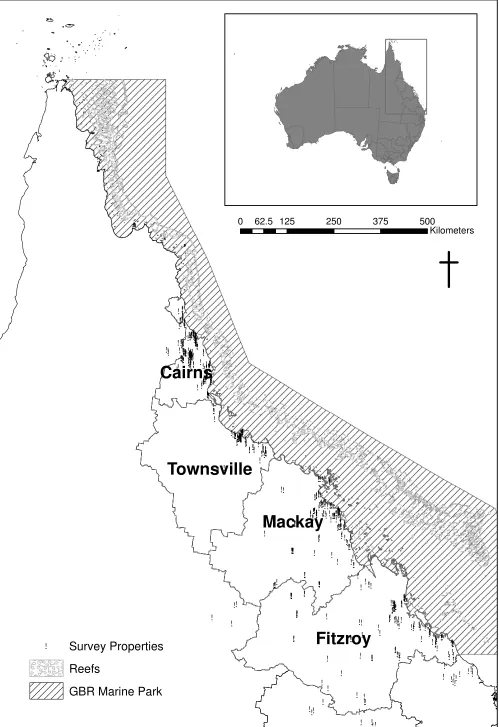
FIGURE 1 MAP FROM SEPARATE EPS FILE TO BE INSERTED HERE
Figure 1 Study area: The Great Barrier Reef World Heritage Area
2.2
Questionnaire design and data collection
LS research assumes that each individual i’s life satisfaction (LSi) is affected by numerous factors
(Xi). Our hypothesis is that these numerous factors include values associated with the CS provided by
the GBR (CSVi), resulting in a conceptual model of the form:
LSi = ƒ (Xi, CSVi) (1)
Our first task, therefore, was to determine how best to measure LSi, Xi and CSVi and how to
empirically estimate the relationship between them.
1 2 3 4 5 6 7 8 9 10 11 12 13 14 15 16 17 18 19 20 21 22 23 24 25 26 27 28 29 30 31 32 33 34 35 36 37 38 39 40 41 42 43 44 45 46 47 48 49 50 51 52 53 54 55 56 57 58 59 60 61
Cantril Ladder (Cantril, 1965)). We chose to use a single question, asking respondents to consider their own life and personal circumstances, and to then indicate, on a 5 point Likert scale, how satisfied they were with life overall.
As regard ‘other’ variables (Xi):, we used a range of socio-demographic and economic variables
informed by those variables which previous researchers have found to be significantly related to LS (a summary of articles using different determinants is provided in Appendix 1). As such, our survey included numerous background questions about age, gender, marital status, income, etc. (Table 2 summarises those variables retained within our final model, Appendix 2 sets out all the variables tested as part of our empirical analysis).
Determining how best to assess CSVi was a little more problemmatic. If wishing to assess the
contribution a standard economic good (say, widgets) makes to overall LS (wellbeing, or utility), one would ideally count the number of widgets consumed by each individual over a given period of time (say one year), and include that in the regression equation. Within an environmental context, if seeking to place a value on conservation activities for a particular species, one could include a measure of population size within the regression. However, this cannot easily be done for CS values (particularly those relating to the non-use elements that comprise a significent portion of total CS), as there is no meaningful way to measure quantity, since the service is either there (for all people) or not. We are seeking to value the benefit of the GBR continuing to exist as opposed to becoming marginally less available, thus we estimate a total value (all or nothing), rather than a marginal value, where the problem of ‘scope’ may be significant2
. Still, it is difficult to determine how to measure this – particularly given the complex inter-relationships between various use and non-use values (or between cultural and other ES). We chose to focus on people’s perceptions of their satisfaction with
2 When estimating marginal values, this can vary depending on the starting point; e.g., people are likely to be
1 2 3 4 5 6 7 8 9 10 11 12 13 14 15 16 17 18 19 20 21 22 23 24 25 26 27 28 29 30 31 32 33 34 35 36 37 38 39 40 41 42 43 44 45 46 47 48 49 50 51 52 53 54 55 56 57 58 59 60 61
numerous ES (and other) values using a coarse Likert scale to gauge ‘satisfaction’ and principal components analysis (PCA)3 to identify items associated with CS.
People’s perceptions were gathered using surveys. The questionnaire included a list of 18 different
community defined benefits representing many different services provided by the GBR (Table 1), developed from a literature review and by consulting regional stakeholders/managers/decision makers during workshops held in Cairns, Brisbane and Townsville (see Stoeckl, Farr, Jarvis, et al. (2014) for details of literature review and workshops). The questionnaire asked, amongst other things, “How satisfied are you with each item below? Indicate whether all is well (very satisfied) or if there is
something wrong (very unsatisfied)”. Responses were recorded on a 5-point scale.
Table 1 Community-defined benefits assessed in the questionnaire
The status/health of the region’s:
*Beaches and islands – undeveloped and uncrowded
*Beaches and islands – without visible rubbish (bottles, plastic)
*Coral reefs
*Reef fish
*Iconic marine species (whales, dugongs, turtles)
*Oceans – clear water (with good underwater visibility)
*Mangroves and wetlands
*The chances that the GBR World Heritage Area will be preserved for future generations
The benefits you receive from:
The reef-based tourism industry
The commercial fishing sector
The mining and agricultural sectors
Cheap shipping transport
The health/status of traditional/indigenous cultural values
The status of your ‘bragging rights’ – knowing that people envy you for living near the Great Barrier Reef
Your opportunities to:
Eat fresh locally caught seafood
Go fishing, spear-fishing or crabbing
3
1 2 3 4 5 6 7 8 9 10 11 12 13 14 15 16 17 18 19 20 21 22 23 24 25 26 27 28 29 30 31 32 33 34 35 36 37 38 39 40 41 42 43 44 45 46 47 48 49 50 51 52 53 54 55 56 57 58 59 60 61
Spend time on the beach, go swimming, diving etc.
Go boating, sailing or jet-skiing
* Benefits included within the composite single variable for CS values as a result of PCA
Some of the community defined benefits listed in Table 1 clearly represented provisioning services. Of these, some were strongly associated with the market and were priced, such as benefiting from the jobs and incomes associated with the commercial fishing industry, whilst others were non-priced e.g. being able to eat fresh locally caught seafood. Other benefits were arguably more strongly associated with CS values (e.g. ‘having’ healthy iconic marine species, reefs and reef fish, knowing that the GBR will be preserved for future generations). At issue here is the problem of deciding which benefit(s) to use as a proxy for CS values.
This is a non-trivial problem; ecosystems are complex, composed of non-linear, interdependent components, and the value of the services they produce are interdependent and overlapping (Costanza et al., 1997). Therefore, we sought to develop a collective measure, combining responses to questions about satisfaction with benefits most closely associated with measures of CS, such collective measures of value having been recommended over single measures (Stoeckl, Farr, Larson, et al., 2014; Windle & Rolfe, 2005).
In the first instance, we checked for separability by looking at correlation coefficients and using PCA (with Varimax rotation and Kaiser normalization), finding that these 18 benefits collapsed into 5 separable factors. The factors, and the benefits which were grouped into each factor resulting from the PCA, along with the factor scores, are set out within Appendix 3. The groupings were the same as those found by Larson, Stoeckl, Farr, and Esparon (2014) and Stoeckl, Farr, Larson, et al. (2014) who grouped the benefits based on importance (rather than satisfaction) scores; thus the groupings appear robust to whichever measure is chosen. Having identified that the responses to 8 of these questions did, in fact, appear to be ‘separable’ to responses about other benefits (the starred variables in Table
1 2 3 4 5 6 7 8 9 10 11 12 13 14 15 16 17 18 19 20 21 22 23 24 25 26 27 28 29 30 31 32 33 34 35 36 37 38 39 40 41 42 43 44 45 46 47 48 49 50 51 52 53 54 55 56 57 58 59 60 61
Importantly, this proxy for CS values focuses on residents’ perceptions and does not consider the
actual condition of the GBR. It is noted, however, that respondent’s perceptions have frequently and successfully been used within LS studies, including perceived water quality (Guardiola, González-Gómez, & Lendechy Grajales, 2013), perceived aircraft noise (van Praag & Baarsma, 2005) and self-assessed perceptions of health (Diener, Suh, Lucas, & Smith, 1999). Relatedly, researchers have found evidence to suggest that perceptions (of water quality) do a better job of explaining willingness to pay (for improvements in water quality), than do objective measures (of water quality) (Farr, Stoeckl, Esparon, Larson, & Jarvis, 2014). Thus, it is our attempt to include a measure of CS values within the LS model that adds something new to the literature; use of perceptions (rather than of objective measures) is neither novel nor controversial.
2.3 Sampling / data collection
24 different versions of the questionnaire were generated – each version presenting the list of benefits (Table 1) in a different order, since survey respondents have been found to be highly sensitive to the order in which questions are presented4 (Cai, Cameron, & Gerdes, 2011; Lasorsa, 2003). Questionnaires were pre-tested amongst colleagues and in a pilot study of 200 residents from 100 different postcodes within the GBR catchment area.
The surveys were mailed out5 (with explanatory letter) to a geographically stratified random selection of households from postcodes that lay either partially or entirely within the GBR catchment area (Figure 1). Only one half of our residents were sent the full questionnaire where they were asked about both importance and satisfaction of the community defined benefits. The remainder were given a shorter questionnaire only covering the importance of these benefits; thus responses to these had to
4 Dummy variables representing the order that the questions were asked were incorporated within an enlarged
form of the overall OLS model developed by this study; as these ‘order of question’ dummy variables were not found to be significant our results do not appear to be influenced by question order. Results available on request.
5 Mail out survey collection was chosen rather than using face to face methods, partly due to time and budget
1 2 3 4 5 6 7 8 9 10 11 12 13 14 15 16 17 18 19 20 21 22 23 24 25 26 27 28 29 30 31 32 33 34 35 36 37 38 39 40 41 42 43 44 45 46 47 48 49 50 51 52 53 54 55 56 57 58 59 60 61
be excluded from this research as the satisfaction responses were at the core of this study. The Dilman (2007) method was followed; recording returned questionnaires as they arrived, sending a replacement questionnaire to those who had not responded shortly after the first contact, and a further replacement shortly after that. We ensured that an equal number of each version of our questionnaires were sent to each postcode to ensure that the order of the questions did not influence our results. We estimate that 3,977 reached their intended recipient and we received 902 completed questionnaires, giving an overall response rate of 22.7%. Of these 902 completed questionnaires, 515 responses were of the longer version of the survey that were usable within this study, and for almost half of
these, 245, the respondent had answered all of the questions required for this analysis6.
2.4
Econometric issues
Previous LS studies have used a range of estimation techniques, some suitable for categorical or ordinal dependent variables (such as Frey & Stutzer, 1999) and others more appropriate for continuous distributions (for example Easterlin, 1995). Research has been conducted into the effect of using techniques designed for continuous rather than ordinal data; the impact has been found to be small, based on statistical literature (Kromrey & Rendina-Gobioff, 2002; Newsom, 2012). Moreover,
insights from the LS research literature (Ferrer‐i‐Carbonell & Frijters, 2004; MacKerron &
Mourato, 2009) suggests that the choice of estimation technique (OLS or ordered probit) has little or no impact on the resulting valuations (Ambrey & Fleming, 2011; Levinson, 2012; Luechinger, 2009; Luechinger & Raschky, 2009). Moreover, as Levinson (2012) points out, the LS approach is based on a ratio of coefficients, rather than the absolute effect on the ordinal dependent ratio; as such final estimates of ‘value’ may be relatively insensitive to the choice of ordinal or continuous techniques;
6 As frequently found with survey based social sciences studies, there is a possibility of sample selection bias; it
1 2 3 4 5 6 7 8 9 10 11 12 13 14 15 16 17 18 19 20 21 22 23 24 25 26 27 28 29 30 31 32 33 34 35 36 37 38 39 40 41 42 43 44 45 46 47 48 49 50 51 52 53 54 55 56 57 58 59 60 61
this conclusion is confirmed by others (Welsch & Kühling, 2009). As such, it appears that the use of continuous techniques may be appropriate.
A more neglected econometric issue is space/location (MacKerron, 2012). Some researchers have used spatially derived data within their analysis including, for example, variables that indicate proximity to features such as the coast, landfill sites, airports, major roads (Brereton, Clinch, & Ferreira, 2008). Researchers have also included measures of climate (specifically rainfall, temperature and wind speed data) (Brereton et al., 2008; Ferreira & Moro, 2010); and local measures of pollution (Luechinger, 2009; MacKerron & Mourato, 2009). But, so far as we are aware, only one study has specifically addressed the issue of spatial variation in the relationship between LS and explanatory variables: Stanca (2010), who sought to determine if the relationships between unemployment, income and LS were ‘similar’ for countries that were geographically close, concluding that “in order to understand the links between economics and happiness, geography
matters” (Stanca, 2010, p. 132). We thus used geographically weighted regression (GWR), a refinement to OLS regression, to estimate our LS model. Our use of GWR is discussed further within Appendix 4.
The final set of variables used in the regression was obtained after a series of estimations; starting from a specification including a wide range of variables suggested by the literature (described within Appendix 1). Insignificant variables were gradually dropped (a list of all the potential explanatory variables tested within the model is set out at Appendix 2). When running these models, we generated a single, OLS ‘global’ model and also used GWR. We tested for the presence of spatial
non-stationarity between explanatory variables and LS with the Koenker BP test, confirming the appropriateness of GWR. Spatial autocorrelation was tested for using the Global Moran’s I test which
indicated that our final model reflected the inherent spatial nature of the data with no important spatial variable having been omitted (thus omitted variable bias is unlikely).
1 2 3 4 5 6 7 8 9 10 11 12 13 14 15 16 17 18 19 20 21 22 23 24 25 26 27 28 29 30 31 32 33 34 35 36 37 38 39 40 41 42 43 44 45 46 47 48 49 50 51 52 53 54 55 56 57 58 59 60 61
respondents in any region, those observations were combined with observations from the adjacent region, thus ensuring that all groupings included a reasonable proportion of the overall sample (ranging from 16% to 34% of the total), therefore no group was so small that an outlying response could significantly distort the region’s average.
Recognising that endogeneity could be present (a common problem with LS studies (Kountouris & Remoundou, 2011; Luechinger, 2009)) (particularly given the potential for simultaneity between our indicators of satisfaction with CS and overall LS), we conducted the Wu-Hausman (Hausman, 1978; Wu, 1973) and Durbin (Durbin, 1954) tests. These tests provided no evidence of its presence, suggesting that the measures of both satisfaction with CS and income are exogenous, and that use of instrumental variables would not be appropriate7.
2.5
Using coefficients from the model to generate a monetary estimate of the value
of cultural ecosystem services
Most LS studies use coefficients from the LS model to calculate the marginal rate of substitution between income and some other variable (e.g. pollution). This is entirely appropriate if working with variables for which marginal changes are possible, but is not appropriate to think about ‘marginal’
changes in quantity when considering the future of a non-rivalrous common-property good such as the GBR; the Reef either will be preserved for future generations, or it will be allowed to deteriorate and die. That said, it IS possible to have marginal changes in quality: it could be preserved in excellent, good, or some other condition. Our proxy for CS values is far from perfect but it does incorporate a measure of people’s perceptions about the state of the region (specifically, satisfaction with the
quality of various aspects of the GBR such as coral reefs, reef fish). Moreover, for the moment we can offer no alternative variable that is both theoretically correct and empirically practical. We thus replicate the estimation process. That is, we estimate the (average) amount of additional income that each respondent would need to adequately compensate them (i.e. to keep overall LS constant) should there be a reduction in their satisfaction with the various CS values associated with the GBR.
1 2 3 4 5 6 7 8 9 10 11 12 13 14 15 16 17 18 19 20 21 22 23 24 25 26 27 28 29 30 31 32 33 34 35 36 37 38 39 40 41 42 43 44 45 46 47 48 49 50 51 52 53 54 55 56 57 58 59 60 61
Average compensation per person =
The included here is that resulting from satisfaction levels falling from current levels to zero. A single estimate of ‘value’ was calculated using the coefficients from the GWR model, and ‘values’
were also estimated for each of the four regions, using the spatially differentiated coefficients to do so. We then multiply this per-capita figure by the number of employed persons in the region, to generate an aggregate estimate of the value of CS8.
3
Results and Discussion
3.1
The estimated regression model
Our analysis uses only a subset of all responses (n=245): those who answered every question, and for which we had enough locational information to identify the latitude and longitude of the residence, so that GWR could be used. The survey respondent’s home locations are indicated in the map at Figure
1 (drawn at a scale that prevents identification of respondents to preserve confidentiality).
The distribution of responses to the question about LS, and the distribution of responses to the questions regarding satisfaction with the cultural ecosystem services (CSV) associated with the GBR are shown in Figure 2, while Table 2 provides summary statistics for the other variables used in the LS model (the X’s)9
.
8
It should be recognised there is no assumption that this compensation be actually offered; neither are we proposing that the residents of the region would be willing to accept a monetary compensation for any degradation in the CS provided by the GBR. Specifically, this calculation has estimated the amount of income that would generate the equivalent impact on LS as that currently provided by the CS that the residents enjoy.
9
1 2 3 4 5 6 7 8 9 10 11 12 13 14 15 16 17 18 19 20 21 22 23 24 25 26 27 28 29 30 31 32 33 34 35 36 37 38 39 40 41 42 43 44 45 46 47 48 49 50 51 52 53 54 55 56 57 58 59 60 61
Figure 2 Responses to questions regarding satisfaction with life overall and with the
cultural ecosystem services values associated with the GBR
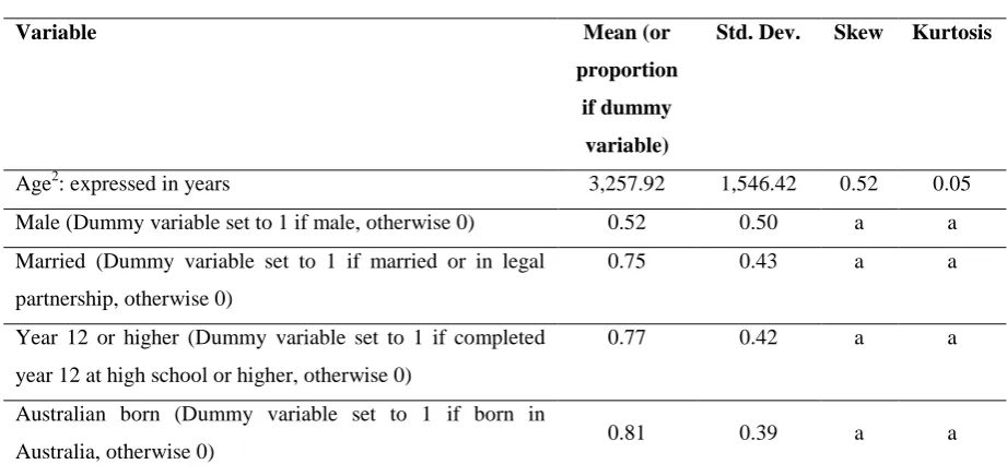
Table 2 Other explanatory variables used in the LS model
Variable Mean (or
proportion if dummy
variable)
Std. Dev. Skew Kurtosis
Age2: expressed in years 3,257.92 1,546.42 0.52 0.05
Male (Dummy variable set to 1 if male, otherwise 0) 0.52 0.50 a a
Married (Dummy variable set to 1 if married or in legal
partnership, otherwise 0)
0.75 0.43 a a
Year 12 or higher (Dummy variable set to 1 if completed
year 12 at high school or higher, otherwise 0)
0.77 0.42 a a
Australian born (Dummy variable set to 1 if born in
Australia, otherwise 0) 0.81 0.39 a a
0% 10% 20% 30% 40% 50% 60% 70% 80% 90% 100% Sat is fact ion with lif e o ve ra ll Be ach es & Is lan d s - u n d ev elop ed /u n crowd ed Be ach es & Is lan d s - w ith o u t vis ib le ru b b is h Cora l re ef s Re ef fi sh Icon ic m ar in e sp ecie s Oce an s - cle ar w at er Ma n grov es an d w etla n d s Pres erv ed f o r fu tu re generat ion s % o f re sp o n se s
[image:17.595.65.526.535.753.2]1 2 3 4 5 6 7 8 9 10 11 12 13 14 15 16 17 18 19 20 21 22 23 24 25 26 27 28 29 30 31 32 33 34 35 36 37 38 39 40 41 42 43 44 45 46 47 48 49 50 51 52 53 54 55 56 57 58 59 60 61
Income: individual income in $10 51,373.27 33,889.68 1.20 2.51 a: skew and kurtosis are not relevant for categorical data.
The results from the OLS, the overall GWR and each of the four models (Cairns, Townsville, Mackay and Fitzroy, in order from north to south) are presented in Table 3.
The Koenker BP Statistic was 13.138 significant at 10% level, indicating that spatial variations are present. The GWR estimation process provided a higher adjusted R2 statistic and a lower AIC than the global OLS model indicating that the GWR models provide better goodness of fit, further confirming the existence of spatial variations. The Global Moran’s I test value was -0.007, not significant even at 10% level; this confirms that spatial autocorrelation is not present in the regression residuals, indicating the model reflects the inherent spatial nature of the data with no important spatial variable having been omitted.
We thus focus on the GWR results, firstly considering the overall model. All explanatory variables were significant at 5% level. The adjusted R2 is fairly low at .140, but is consistent with previous LS research.
The signs and statistical significance of socio-demographic variables were as expected from the literature:
age had a statistically significant and positive relationship with LS (Ambrey & Fleming, 2014; MacKerron & Mourato, 2009);
females were, on average, more satisfied with life than male respondents as were those who were married or in legal partnership (Brereton et al., 2008; Ferrer-i-Carbonell & Gowdy, 2007);
10 For this study survey respondents were asked the question “On average, how much pre-tax income does your
1 2 3 4 5 6 7 8 9 10 11 12 13 14 15 16 17 18 19 20 21 22 23 24 25 26 27 28 29 30 31 32 33 34 35 36 37 38 39 40 41 42 43 44 45 46 47 48 49 50 51 52 53 54 55 56 57 58 59 60 61
those who had completed year 12 education or above were more satisfied than those who had not (Frey & Stutzer, 2000), although we note that the coefficient may also be incorporating the indirect effect that education has on improving health (Dolan, Peasgood, & White, 2008);
those born in Australia had higher LS than migrants (confirming earlier research that found living within your country of origin increases LS (Frey & Stutzer, 1999));
income had a significant and positive impact on LS (Ferreira & Moro, 2010;
Ferrer‐i‐Carbonell & Frijters, 2004).
Our proxy for CS values was highly significant. We are not aware of previous research that has considered the interaction between CS values and overall LS; however, a positive relationship has been found between LS and sustainable development (Zidanšek, 2007), ecosystem diversity (Ambrey & Fleming, 2014), and being concerned about the extinction of species (Ferrer-i-Carbonell & Gowdy, 2007). Thus, the finding that the ES are important to LS accords with our expectations and with findings from studies in a similar field.
For the regional models, the R2 is highest for the most northern region (Cairns) followed by Townsville and then the other regions. This indicates that the model does a slightly better job explaining the relationship between the independent variables and overall LS in the north than the south.
Table 3 GWR and OLS model results for dependent variable: Satisfaction with Life
Overall
GWR model Cairns
GWR model Townsville
GWR model Mackay
GWR model Fitzroy
GWR model Overall
OLS global model Variables Coefficients
Standard errors in brackets
Age2 .00014***
(.00004)
.00014***
(.00004)
.00014***
(.00004)
.00015***
(.00004)
.00014***
(.00004)
.00015***
(.00004)
Male -.3447***
(.1208)
-.2879**
(.1117)
-.2320**
(.1117)
-.2014*
(.1251)
-.2727**
(.1179)
-.2790**
1 2 3 4 5 6 7 8 9 10 11 12 13 14 15 16 17 18 19 20 21 22 23 24 25 26 27 28 29 30 31 32 33 34 35 36 37 38 39 40 41 42 43 44 45 46 47 48 49 50 51 52 53 54 55 56 57 58 59 60 61
Married .5143***
(.1394) .3828*** (.1279) .2333* (.1265) .0985 (.1429) .3232** (.1349) .3073** (.1237)
Year 12 or
higher .5295*** (.1511) .4788*** (.1403) .4033*** (.1403) .3199** (.1576) .4398*** (.1480) .4231*** (.1375) Australian born .4863*** (.1538) .3664** (.1426) .2286 (.1428) .1267 (.1654) .3162** (.1517) .3204** (.1388)
Income 3.012E-06
(2.012E-06) 3.000E-06 (2.000E-06) 4.000E-06** (2.000E-06) 4.857E-06** (2.000E-06) 3.694E-06* (2.004E-06) 4.000E-06** (2.000E-06)
CSV .1412**
(.0614) .1351** (.0572) .1314** (.0575) .1352** (.0655) .1362** (.0606) .1467*** (.0561)
Constant -.5223
(.3108) -.3180 (.2857) -.0826 (.2838) .0752 (.3216) -.2357 (.3020) -.2559 (.2777)
Sample size 84 40 65 56 245 245
Adjusted R2 .140 .113
Local R2 .178 .146 .121 .119
AIC 603.034 608.375
*** p<0.01, ** p<0.05, * p<0.1
Coefficients also vary across models/regions, with a distinct north/south pattern. Income contributes relatively less to overall LS in the north than in the south: indeed it is not even a significant contributor to overall LS in the two most northern regions11. The contribution of other variables is generally greater in the north than the south. This is so for CSV: the models indicate that they are a more important contributor to overall LS for residents of the north than of those in the south.
Tukey Post Hoc tests12 confirmed the statistical significance (at the 1% level) of differences between each coefficient for each region with three exceptions: (i) the coefficient for age squared for Fitzroy was significantly different to all other regions, however Cairns and Townsville, and Townsville and Mackay, did not have significant differences, and the coefficients for Cairns and Mackay were only significantly different at the 5% level (ii) the coefficient for income was not significantly different between Cairns and Townsville, and (iii) the coefficient on CSV was not significantly different between Mackay and Fitzroy.
11 Average incomes of respondents were also higher in the southern regions compared to the north.
12 Post hoc tests that do not assume equal variances were also tested (Tamhane’s T2 test, Dunnett’s T3 test,
1 2 3 4 5 6 7 8 9 10 11 12 13 14 15 16 17 18 19 20 21 22 23 24 25 26 27 28 29 30 31 32 33 34 35 36 37 38 39 40 41 42 43 44 45 46 47 48 49 50 51 52 53 54 55 56 57 58 59 60 61
Visual inspection of Figure 1 clearly shows that some of our respondents reside much closer to the coast, and thus the GBR, than others. Virtually all of our sampled properties within Townsville region were very close to the coast; those of Cairns region were also fairly close, although many respondents were further inland on the Atherton Tablelands. However, the survey respondents within Mackay and Fitzroy regions are widely dispersed, respondents from the southern part of the study area were, on average, more than 2.5 times further from the coast than those from the northern section. An inverse relationship is generally expected between protection values applied to environmental assets and distance from the asset, referred to as distance decay (Rolfe & Windle, 2012). Theory suggests that the rate of decay would vary across different ES. Recognising that geographical proximity to the Reef may impact results, a variable measuring proximity to the Reef was included within the regressions. This variable was not significant, suggesting distance decay is not an issue. This confirms observation from other studies of values in the GBR region (Rolfe & Windle, 2012) and accords with theory that distance decay would be small or even zero for non-use values for a unique feature (Pascual et al., 2010) as the GBR is indeed unique and a large component of the total CS value is likely to relate to non-use values.
3.2
Estimating the valuation of cultural ecosystem services provided by the GBR
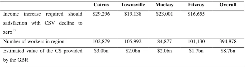
Table 4 presents our estimates of the additional income that would be required to compensate residents should current (median) levels of satisfaction with CS values drop to zero (equivalent to a situation where residents are neither satisfied nor dissatisfied). These range from almost $30k per capita per annum for Cairns to $17k - $23k per annum per capita in the other regions. Multiplying this amount by the number of employed persons in the GBR region, being 394,878 in total (Australian Bureau of Statistics, 2011), suggests that aggregate ‘regional’ compensation, representing the CS value of the GBR, would be about $8.7 billion per annum. Whilst some studies have attempted to estimate marginal non-use values in the GBR (see, for example the research of Rolfe and colleagues),
1 2 3 4 5 6 7 8 9 10 11 12 13 14 15 16 17 18 19 20 21 22 23 24 25 26 27 28 29 30 31 32 33 34 35 36 37 38 39 40 41 42 43 44 45 46 47 48 49 50 51 52 53 54 55 56 57 58 59 60 61
[image:22.595.66.533.191.320.2]predicted that this group of mainly non-use CS would be worth more than $4 billion per annum associated with the GBR based tourism industry; our results are not inconsistent with theirs.
Table 4 Estimated value of CS provided by the GBR to residents of the regions and
overall
Cairns Townsville Mackay Fitzroy Overall
Income increase required should
satisfaction with CSV decline to
zero13
$29,296 $19,138 $23,001 $16,655
Number of workers in region 102,879 105,992 84,877 101,130 394,878
Estimated value of the CS provided
by the GBR
$3.0bn $2.0bn $2.0bn $1.7bn $8.7bn
It should be noted that although the coefficient on income is significant overall, and significant within the Mackay and Fitzroy regions, it was not significant in the Cairns or Townsville regions. This result could be interpreted to mean that there is no amount of income that could adequately recompense the residents of these regions should the CS cease to satisfy them; that is the CS is ‘priceless’ to the
residents of those regions. In accordance with the law of diminishing marginal utility, once income reaches a certain level then further increases to income will only have a very small impact on utility; the insignificant income coefficients found here indicate that for many of the residents in the northern regions this position may have been reached and thus additional income is unable to compensate for the loss of another benefit (the CS of the GBR) which contributes significantly towards LS. Furthermore, the finding of an insignificant coefficient for income in explaining LS (which results in the large value assigned to CS) in these regions is not unique to this study (and hence should not be dismissed as a function of a weakness in the study); indeed, this is the core of Easterlin’s income paradox (Easterlin, 1973).
13
1 2 3 4 5 6 7 8 9 10 11 12 13 14 15 16 17 18 19 20 21 22 23 24 25 26 27 28 29 30 31 32 33 34 35 36 37 38 39 40 41 42 43 44 45 46 47 48 49 50 51 52 53 54 55 56 57 58 59 60 61
This research has clearly identified spatial variations in the value placed on CS, that is, CS are relatively more important to LS for residents in the north whilst income is relatively more important to LS for those in the south. However, cross-sectional research cannot identify the causality within this relationship: does increased incomes cause someone to value money more and place less value on CS? Or do higher paying regions attract residents who value money relatively highly, whilst regions offering more/better quality CS attract residents who value CS relatively highly? Future research
using time-series or panel data could usefully illuminate this important question.
4
Conclusions
This research seeks to extend the existing literature based on the LS approach to environmental valuation. Using the GBR as a case study we have tested if it is, in principle, possible to use this technique to estimate the value of the CS provided by an environmental feature. Our findings are cautiously affirmative – although we stress the need for much further research on methods of using
questionnaires to measure CS for use in LS studies.
1 2 3 4 5 6 7 8 9 10 11 12 13 14 15 16 17 18 19 20 21 22 23 24 25 26 27 28 29 30 31 32 33 34 35 36 37 38 39 40 41 42 43 44 45 46 47 48 49 50 51 52 53 54 55 56 57 58 59 60 61
5
Acknowledgments
This research was conducted with the support of funding from the Tropical Ecosystems Hub of the Australian Government’s National Environmental Research Program (Project 10.2).
6
References
Ambrey, C. L., & Fleming, C. M. (2011). Valuing scenic amenity using life satisfaction data.
Ecological Economics, 72
, 106-115. doi:10.1016/j.ecolecon.2011.09.011
Ambrey, C. L., & Fleming, C. M. (2014). Valuing Ecosystem Diversity in South East
Queensland: A Life Satisfaction Approach.
Social Indicators Research, 115
(1),
45-65. doi:10.1007/s11205-012-0208-4
Australian Bureau of Statistics. (2010). 1287.0 Standards for Income Variables 2010.
Retrieved
from
http://www.abs.gov.au/AUSSTATS/[email protected]/Lookup/ED44B2BCB1995523CA2576
E40014561A?opendocument
Australian Bureau of Statistics. (2011). Data by Region. Retrieved from
http://stat.abs.gov.au/itt/r.jsp?databyregion#/
Bateman, I. J., Jones, A. P., Lovett, A. A., Lake, I. R., & Day, B. H. (2002). Applying
geographical information systems (GIS) to environmental and resource economics.
Environmental
&
Resource
Economics,
22
(1/2),
219-269.
doi:10.1023/A:1015575214292
Braat, L. C., & de Groot, R. (2012). The ecosystem services agenda:bridging the worlds of
natural science and economics, conservation and development, and public and private
policy. Ecosystem Services, 1(1), 4-15. doi:10.1016/j.ecoser.2012.07.011
Brereton, F., Clinch, J. P., & Ferreira, S. (2008). Happiness, geography and the environment.
Ecological Economics, 65
(2), 386-396. doi:10.1016/j.ecolecon.2007.07.008
Cai, B., Cameron, T. A., & Gerdes, G. R. (2011). Distal order effects in stated preference
surveys.
Ecological
Economics,
70
(6),
1101-1108.
doi:10.1016/j.ecolecon.2010.12.018
Cantril, H. (1965).
Pattern of human concerns
. New Brunswick, New Jersey: Rutgers
University Press.
Carbone, J. C., & Kerry Smith, V. (2013). Valuing nature in a general equilibrium.
Journal of
Environmental
Economics
and
Management,
66
(1),
72-89.
doi:10.1016/j.jeem.2012.12.007
Carson, R. T., Flores, N. E., & Meade, N. F. (2001). Contingent valuation: controversies and
evidence.
Environmental
&
Resource
Economics,
19
(2),
173-210.
doi:10.1023/A:1011128332243
Costanza, R. (2006). Nature: ecosystems without commodifying them.
Nature, 443
(7113),
749-749. doi:10.1038/443749b
Costanza, R., d'Arge, R., de Groot, R., Farber, S., Grasso, M., Hannon, B., . . . O'Neill, R. V.
(1997). The value of the world's ecosystem services and natural capital.
Nature, 387
,
253-260.
1 2 3 4 5 6 7 8 9 10 11 12 13 14 15 16 17 18 19 20 21 22 23 24 25 26 27 28 29 30 31 32 33 34 35 36 37 38 39 40 41 42 43 44 45 46 47 48 49 50 51 52 53 54 55 56 57 58 59 60 61
well-being.
Ecological
Economics,
61
(2),
267-276.
doi:10.1016/j.ecolecon.2006.02.023
Daily, G. C., Söderqvist, T., Aniyar, S., Arrow, K., Dasgupta, P., Ehrlich, P. R., . . . Walker,
B. (2000). The Value of Nature and the Nature of Value.
Science, 289
(5478),
395-396. doi:10.1126/science.289.5478.395
Daw, T. M., Coulthard, S., William, W. L. C., Brown, K., Abunge, C., Galafassi, D., . . .
Stockholm Resilience, C. (2015). Evaluating taboo trade-offs in ecosystems services
and human well-being.
Proceedings of the National Academy of Sciences, 112
(22),
6949-6954. doi:10.1073/pnas.1414900112
de Groot, R., Brander, L., van der Ploeg, S., Costanza, R., Bernard, F., Braat, L., . . . van
Beukering, P. (2012). Global estimates of the value of ecosystems and their services
in monetary units.
Ecosystem Services, 1
(1), 50-61. doi:10.1016/j.ecoser.2012.07.005
de Groot, R., Fisher, B., Christie, M., Aronson, J., Braat, L., Gowdy, J., . . . Ring, I. (2010).
Integrating the ecological and economic dimensions in biodiversity and ecosystem
service valuation (Chapter 1) In: Kumar, P.(Ed.),(2010) TEEB Foundations, The
Economics of Ecosystems and Biodiversity: Ecological and Economic Foundations.
Earthscan, London
.
De’ath, G., Fabricius, K. E., Sweatman, H., & Puotinen, M. (2012). The 27–year decline of
coral cover on the Great Barrier Reef and its causes.
Proceedings of the National
Academy of Sciences, 109
(44), 17995-17999.
Diener, E., Suh, E. M., Lucas, R. E., & Smith, H. L. (1999). Subjective Well-Being: Three
Decades of Progress.
Psychological Bulletin, 125
(2), 276-302.
doi:10.1037/0033-2909.125.2.276
Dilman, D. A. (2007).
Mail and Internet surveys: the tailored design, —2007 update
. San
Fransisco: John Wiley.
Dolan, P., Peasgood, T., & White, M. (2008). Do we really know what makes us happy?: a
review of the economic literature on the factors associated with subjective well-being.
Journal of economic psychology, 29
(1), 94-122. doi:10.1016/j.joep.2007.09.001
Durbin, J. (1954). Errors in Variables.
Revue de l'Institut International de Statistique / Review
of the International Statistical Institute, 22
(1/3), 23-32.
Easterlin, R. A. (1973). Does money buy happiness.
Public Interest
(30), 3-10.
Easterlin, R. A. (1995). Will raising the incomes of all increase the happiness of all?
Journal
of Economic Behavior and Organization, 27
(1), 35-47.
doi:10.1016/0167-2681(95)00003-B
Engelbrecht, H.-J. (2009). Natural capital, subjective well-being, and the new welfare
economics of sustainability: Some evidence from cross-country regressions.
Ecological Economics, 69
(2), 380-388. doi:10.1016/j.ecolecon.2009.08.011
Farr, M., Stoeckl, N., Esparon, M., Larson, S., & Jarvis, D. (2014). The importance of water
clarity to tourists in the Great Barrier Reef and their willingness to pay to improve it.
Tourism Economics Fast Track
. doi:http://dx.doi.org/10.5367/te.2014.0426
Ferreira, S., & Moro, M. (2010). On the use of subjective well-being data for environmental
valuation.
Environmental
&
Resource
Economics,
46
(3),
249-273.
doi:10.1007/s10640-009-9339-8
Ferrer-i-Carbonell, A., & Gowdy, J. M. (2007). Environmental degradation and happiness.
Ecological Economics, 60
(3), 509-516. doi:10.1016/j.ecolecon.2005.12.005
1 2 3 4 5 6 7 8 9 10 11 12 13 14 15 16 17 18 19 20 21 22 23 24 25 26 27 28 29 30 31 32 33 34 35 36 37 38 39 40 41 42 43 44 45 46 47 48 49 50 51 52 53 54 55 56 57 58 59 60 61
Frey, B. S., & Stutzer, A. (1999). Measuring Preferences by Subjective Well-Being.
Journal
of Institutional and Theoretical Economics (JITE) / Zeitschrift für die gesamte
Staatswissenschaft, 155
(4), 755-778.
Frey, B. S., & Stutzer, A. (2000). Happiness, Economy and Institutions.
The Economic
Journal, 110
(466), 918-938. doi:10.1111/1468-0297.00570
Furnas, M. (2003).
Catchments and corals: terrestrial runoff to the Great Barrier Reef
.
Townsville, Qld: Australian Institute of Marine Science.
Gómez-Baggethun, E., de Groot, R., Lomas, P. L., & Montes, C. (2010). The history of
ecosystem services in economic theory and practice: From early notions to markets
and
payment
schemes.
Ecological
Economics,
69
(6),
1209-1218.
doi:10.1016/j.ecolecon.2009.11.007
Gómez-Baggethun, E., & Ruiz-Pérez, M. (2011). Economic valuation and the
commodification of ecosystem services.
Progress in Physical Geography, 35
(5),
613-628. doi:10.1177/0309133311421708
Gowdy, J. M. (2005). Toward a new welfare economics for sustainability.
Ecological
Economics, 53
(2), 211-222. doi:10.1016/j.ecolecon.2004.08.007
Guardiola, J., González-Gómez, F., & Lendechy Grajales, Á. (2013). The Influence of Water
Access in Subjective Well-Being: Some Evidence in Yucatan, Mexico.
Social
Indicators Research, 110
(1), 207-218. doi:10.1007/s11205-011-9925-3
Haines-Young, R., & Potschin, M. (2013).
Common International Classification of
Ecosystem Services (CICES): Consultation on Version 4, August-December 2012.
EEA Framework Contract No EEA/IEA/09/003 Download at www.cices.eu or
www.nottingham.ac.uk/cem
. Retrieved from
Hausman, J. A. (1978). Specification Tests in Econometrics.
Econometrica, 46
(6),
1251-1271.
Hundloe, T., Vanclay, F., & Carter, M. (1987).
Economic and socio-economic impacts of the
crown of thorns starfish on the Great Barrier Reef
. Retrieved from
http://marineecosystemservices.org/node/7864
Kountouris, Y., & Remoundou, K. (2011). Valuing the welfare cost of forest fires: a life
satisfaction approach.
Kyklos, 64
(4), 556-578. doi:10.1111/j.1467-6435.2011.00520.x
Kristoffersen, I. (2010). The metrics of subjective wellbeing: cardinality, neutrality and
additivity.
The
economic
record,
86
(272),
98-123.
doi:10.1111/j.1475-4932.2009.00598.x
Kromrey, J. D., & Rendina-Gobioff, G. (2002). An empirical comparison of regression
analysis strategies with discrete ordinal variables.
Multiple linear regression
viewpoints, 28
(2), 30-43.
Kroon, F. J., Kuhnert, P. M., Henderson, B. L., Wilkinson, S. N., Kinsey-Henderson, A.,
Abbott, B., . . . Turner, R. D. R. (2012). River loads of suspended solids, nitrogen,
phosphorus and herbicides delivered to the Great Barrier Reef lagoon.
Marine
pollution bulletin, 65
(4-9), 167. doi:10.1016/j.marpolbul.2011.10.018
Krutilla, J. V. (1967). Conservation Reconsidered.
The American Economic Review, 57
(4),
777-786.
Larson, S., Stoeckl, N., Farr, M., & Esparon, M. (2014). The role the Great Barrier Reef plays
in resident wellbeing and implications for its management.
Ambio
.
Lasorsa, D. L. (2003). Question-order effects in surveys: the case of political interest, news
attention, and knowledge.
Journalism & Mass Communication Quarterly, 80
(3),
499-512. doi:10.1177/107769900308000302
Levinson, A. (2012). Valuing public goods using happiness data: the case of air quality.
1 2 3 4 5 6 7 8 9 10 11 12 13 14 15 16 17 18 19 20 21 22 23 24 25 26 27 28 29 30 31 32 33 34 35 36 37 38 39 40 41 42 43 44 45 46 47 48 49 50 51 52 53 54 55 56 57 58 59 60 61
Lewis, S. E., Brodie, J. E., Bainbridge, Z. T., Rohde, K. W., Davis, A. M., Masters, B. L., . . .
Schaffelke, B. (2009). Herbicides: A new threat to the Great Barrier Reef.
Environmental Pollution, 157
(8), 2470-2484. doi:10.1016/j.envpol.2009.03.006
Luechinger, S. (2009). Valuing Air Quality Using the Life Satisfaction Approach.
The
Economic Journal, 119
(536), 482-515. doi:10.1111/j.1468-0297.2008.02241.x
Luechinger, S., & Raschky, P. A. (2009). Valuing flood disasters using the life satisfaction
approach.
Journal
of
Public
Economics,
93
(3),
620-633.
doi:10.1016/j.jpubeco.2008.10.003
MacKerron, G. (2012). Happiness economics from 35000 feet.
Journal of economic surveys,
26
(4), 705-735. doi:10.1111/j.1467-6419.2010.00672.x
MacKerron, G., & Mourato, S. (2009). Life satisfaction and air quality in London.
Ecological
Economics, 68
(5), 1441-1453. doi:10.1016/j.ecolecon.2008.10.004
Maddison, D., & Rehdanz, K. (2011). The impact of climate on life satisfaction.
Ecological
Economics, 70
(12), 2437-2445. doi:10.1016/j.ecolecon.2011.07.027
Martin-Lopez, B., Gomez-Baggethun, E., Garcia-Llorente, M., & Montes, C. (2014).
Trade-offs across value-domains in ecosystem services assessment.
Ecological Indicators,
37
, 220-228. doi:10.1016/j.ecolind.2013.03.003
Millennium Ecosystem Assessment. (2005).
Ecosystems and human well-being: general
synthesis
. Washington, DC: Island Press.
Newsom, J. (2012). Regression models for Ordinal Dependent Variables, Data Analysis 11,
Fall
2012,
Portland
State
University.
Retrieved
from
http://www.upa.pdx.edu/IOA/newsom/da2/ho_ordinal.pdf
Pascual, U., Muradian, R., Brander, L., Gómez-Baggethun, E., Martín-López, B., Verma, M.,
. . . Eppink, F. (2010). The economics of valuing ecosystem services and biodiversity
(Chapter 5) In: Kumar, P.(Ed.),(2010) TEEB Foundations, The Economics of
Ecosystems and Biodiversity: Ecological and Economic Foundations.
Earthscan,
London
.
Rolfe, J., & Windle, J. (2012). Distance decay functions for iconic assets: assessing national
values to protect the health of the Great Barrier Reef in Australia.
Environmental &
Resource Economics, 53
(3), 347-365. doi:10.1007/s10640-012-9565-3
Stanca, L. (2010). The Geography of Economics and Happiness: Spatial Patterns in the
Effects of Economic Conditions on Well-Being.
Social Indicators Research, 99
(1),
115-133. doi:10.1007/s11205-009-9571-1
Stoeckl, N., Farr, M., Jarvis, D., Larson, S., Esparon, M., Sakata, H., . . . Costanza, R. (2014).
The Great Barrier Reef World Heritage Area: its ‘value’ to residents and tourists
Project 10-2 Socioeconomic systems and reef resilience. Final Report to the National
Environmental Research Program. Reef and Rainforest Research Centre Limited
.
Retrieved from Cairns:
Stoeckl, N., Farr, M., Larson, S., Adams, V., Kubiszewski, I., Esparon, M., & Costanza, R.
(2014). A new approach to the problem of overlapping values: A case study in
Australia's Great Barrier Reef.
Ecosystem Services, 10
, 61-78.
Stoeckl, N., Hicks, C. C., Mills, M., Fabricius, K., Esparon, M., Kroon, F., . . . Costanza, R.
(2011). The economic value of ecosystem services in the Great Barrier Reef: our state
of knowledge in "Ecological Economics Reviews".
Annals of the New York Academy
of Sciences
(1219), 113-133.
UNESCO World Heritage Centre. (2014). Decision on status of Australia's Great Barrier
Reef deferred until 2015. Retrieved from http://whc.unesco.org/en/news/1149
1 2 3 4 5 6 7 8 9 10 11 12 13 14 15 16 17 18 19 20 21 22 23 24 25 26 27 28 29 30 31 32 33 34 35 36 37 38 39 40 41 42 43 44 45 46 47 48 49 50 51 52 53 54 55 56 57 58 59 60 61
van Praag, B. M. S., & Baarsma, B. E. (2005). Using happiness surveys to value intangibles:
The case of airport noise.
The Economic Journal, 115
(500), 224-246.
Weisbrod, B. A. (1964). Collective-Consumption Services of Individual-Consumption
Goods.
The Quarterly Journal of Economics, 78
(3), 471-477.
Welsch, H., & Kühling, J. (2009). Using happiness data for environmental valuation: issues
and applications.
Journal of economic surveys, 23
(2), 385-406.
doi:10.1111/j.1467-6419.2008.00566.x
Windle, J., & Rolfe, J. (2005). Assessing Non-use Values for Environmental Protection of an
Estuary in a Great Barrier Reef Catchment.
Australasian Journal of Environmental
Management, 12
(3), 147-155.
Wu, D.-M. (1973). Alternative Tests Of Independence Between Stochastic Regressors And
Disturbances: 1. Introduction.
Econometrica (pre-1986), 41
(4), 733.
1 2 3 4 5 6 7 8 9 10 11 12 13 14 15 16 17 18 19 20 21 22 23 24 25 26 27 28 29 30 31 32 33 34 35 36 37 38 39 40 41 42 43 44 45 46 47 48 49 50 51 52 53 54 55 56 57 58 59 60 61
New methods for valuing, and for identifying spatial
variations, in cultural services: A case study of the
Great Barrier Reef
Appendix 1: Factors frequently found to explain variations in Life
Satisfaction (LS)
Factors frequently
found in studies
Relationship generally found with LS
Age Either positive (Ambrey & Fleming, 2014; MacKerron & Mourato, 2009) or U
shaped (Di Tella, MacCulloch, & Oswald, 2003). Potential non-linearity addressed
by including age and/or age squared.
Gender Females have higher SWB (Brereton, Clinch, & Ferreira, 2008; Ferreira et al.,
2013; Ferrer-i-Carbonell & Gowdy, 2007; Welsch, 2007b).
Marital status Marriage increases LS; divorce associated with lower SWB (Diener, Suh, Lucas, &
Smith, 1999).
Living in country of
origin (not a foreigner)
Improves SWB (Frey & Stutzer, 1999).
Employed rather than
unemployed
Improves SWB (Winkelmann & Winkelmann, 1998); living in high unemployment
region, even if not unemployed, reduces SWB (Welsch, 2007b).
Health Better health improves LS; stronger relationship from subjective rather than
objective health measures (Diener et al., 1999).
Higher incomes Increase SWB (Di Tella et al., 2003; Ferreira & Moro, 2010; Ferrer‐i‐Carbonell &
Frijters, 2004; Welsch, 2002), but alternate research found a negligible/statistically
insignificant relationship (Easterlin, 1995), and recent research has begun to
investigate potential endogeneity issues. Relative income (both to others and to
previous periods) (Easterlin, 1995, 2003), future material aspirations and their
relationship to anticipated future income levels (Easterlin, 1995, 2001), and
previous income levels (reflecting habituation effect) (Menz & Welsch, 2010) may
be important.
Appendices
1 2 3 4 5 6 7 8 9 10 11 12 13 14 15 16 17 18 19 20 21 22 23 24 25 26 27 28 29 30 31 32 33 34 35 36 37 38 39 40 41 42 43 44 45 46 47 48 49 50 51 52 53 54 55 56 57 58 59 60 61
Factors frequently
found in studies
Relationship generally found with LS
Higher education
levels
Increases LS (Frey & Stutzer, 2000). However effect may be indirect as increased
education is likely to increase incomes (Diener et al., 1999) and/or education has an
indirect impact on improving health; education appears to be more important when
health is excluded from studies (Dolan, Peasgood, & White, 2008).
Quality of social
capital
Improves SWB; includes measures such as political stability (Abdallah, Thompson,
& Marks, 2008), degree of freedom and personal choice (Stanca, 2010), and trust in
others or society (Engelbrecht, 2009).
Climatic and
environmental factors
Extreme climates (Frijters & Praag, 1998; Maddison & Rehdanz, 2011), pollution,
including air pollution (MacKerron & Mourato, 2009; Welsch, 2007a) and noise
levels (van Praag & Baarsma, 2005), and environmental disasters, such as draught
(Carroll, Frijters, & Shields, 2009), forest fires (Kountouris & Remoundou, 2011)
and flooding (Luechinger & Raschky, 2009) reduce SWB. SWB is enhanced by
high quality environmental amenities, such as living near the coast or having good
views (Ambrey & Fleming, 2011; Brereton et al., 2008), ecosystem diversity
(Ambrey & Fleming, 2014), the quality of ecosystem services (Abdallah et al.,
2008; Vemuri & Costanza, 2006), and environmental sustainability (Zidanšek,
2007).
Genetic factors Studies of identical and non-identical twins and siblings have established that
genetic/hereditary factors are key determinants of LS and ‘happiness (Lyubomirsky,
Sheldon, & Schkade, 2005; Zidanšek, 2007). Genetic factors have been estimated
to explain between 39% and 58% (Tellegen et al., 1988) and between 40% and 55%
(Diener et al., 1999) of differences; in young children (Braungart, Plomin, DeFries,
& Fulker, 1992) the estimated influence of genetic factors is between 35% and
1 2 3 4 5 6 7 8 9 10 11 12 13 14 15 16 17 18 19 20 21 22 23 24 25 26 27 28 29 30 31 32 33 34 35 36 37 38 39 40 41 42 43 44 45 46 47 48 49 50 51 52 53 54 55 56 57 58 59 60 61
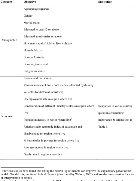
Appendix 2: List of potential explanatory variables tested within the model
Category Objective Subjective
Demographic
Age and age squared
Gender
Marital status
Educated to year 12 or above
Educated at university or above
How many adults/children live with you
Household size
Born in Australia
Born in Queensland
Indigenous status
Economic
Income and Ln Income1
Various sources of household income (denoted by dummy
variables for different industries)
Unemployment rate in region wh