How low can you go? Performance of factor analytic models in the analysis of multi-environment trials with small numbers of varieties

(1)

UNIVERSITY OF SOUTHERN QUEENSLAND

HOW LOW CAN YOU GO? PERFORMANCE OF

FACTOR ANALYTIC MODELS IN THE ANALYSIS OF

MULTI-ENVIRONMENT TRIALS WITH SMALL

NUMBERS OF VARIETIES

Bethany Macdonald B.Sc.

Faculty of Sciences,

The University of Southern Queensland

March 2018

(2)

(3)

©

by

(4)

CERTIFICATION OF DISSERTATION

I certify that the ideas, experimental work, results, analyses, software and conclusions reported in this dissertation are entirely my own effort, except where otherwise acknowl-edged. I also certify that the work is original and has not been previously submitted for any other award, except where otherwise acknowledged.

Bethany Macdonald Date

Endorsement

(5)

Abstract

Crop breeding programs test large numbers of crop varieties in field trials span-ning a range of years and locations, with these groups of trials known as multi-environment trials (MET). In the early stages of crop breeding programs large numbers of new varieties are grown in a small number of field trials. The best varieties in each stage are selected to progress to the next stage so that in the final stages a small number of elite varieties are grown in a large number of field trials across the country. These trials are conducted to determine which varieties per-form best in which environments and an appropriate statistical analysis resulting in accurate predictions of the variety by environment (VxE) effects is integral to this.

There have been many statistical approaches to the analysis of MET data, however all methods involve investigating the nature of the VxE effects. The factor analytic (FA) structure for the VxE effects allows heterogeneity of genetic variance for environments and heterogeneity of genetic covariance between pairs of environments, and is currently considered best practice in the analysis of MET data in Australia. The FA model has been shown to be the superior model for large numbers of varieties both in terms of goodness-of-fit and the selection of su-perior varieties. However, this susu-periority has not been demonstrated for small numbers of varieties, such as in the late stages of crop breeding programs, despite being regularly used in such scenarios. Five data sets with different underlying VxE patterns and numbers of trials, four numbers of varieties, and two levels of varietal concurrence were used to provide scenarios for a simulation study to investigate the adequacy of an FA variance structure for VxE effects. How the accuracy of the FA model changes as the number of crop varieties decrease, along with the implications the underlying VxE variance structure and level of varietal concurrence have on the accuracy of the FA model when dealing with small numbers of varieties were investigated. The comparisons were based on the mean square error of prediction of the VxE effects.

(6)

(7)

Acknowledgements

I would like to thank the following people and organisations for their contribu-tions toward my Honours project:

A huge thank you to Dr. Rachel King and Dr. Alison Kelly for their super-vision, guidance and advice. Their support was invaluable and made my year much less stressful than it could have been.

Col Douglas, Merrill Ryan, and Kristy Hobson for the use of their data.

(8)

(9)

List of Tables

2.1 Summary of data sets used as sources of parameter estimates for data simulation. . . 26 2.2 Summary of models used to analyse selected data sets, showing

the number of parameters estimated in the model (n), the Akaike information criterion (AIC), given here as the difference between the model and the model with the smallest AIC in each data set, the log-likelihood (Logl), and percent of genetic variance accounted for by the FA components in the model (% vaf).. . . 28 2.3 Analysis summary of mungbean data set, showing estimated trial

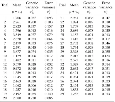
means, genetic variances and error variances. . . 30 2.4 Analysis summary of Desi chickpea data set, showing estimated

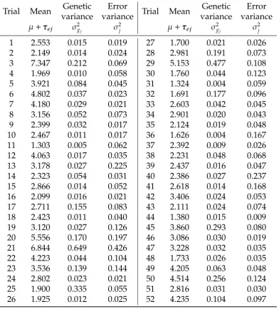
trial means, genetic variances and error variances. . . 30 2.5 Analysis summary of Kabuli chickpea data set, showing estimated

trial means, genetic variances and error variances. . . 31 2.6 Analysis summary of wheat data set, showing estimated trial

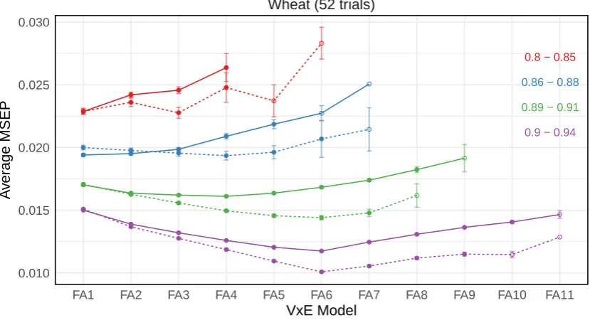
means, genetic variances and error variances. . . 32 2.7 Summary of barley data set from Kellyet al. (2007), showing

esti-mated trial means, genetic variances and error variances. . . 36 3.1 Percentage of simulations in which the unstructured model

con-verged in 500 simulations for mungbean and barley data sets. . . . 45 3.2 Percent of simulations in which model was best according to the

MSEP and log-likelihood ratio test (LLRT) for 500 simulations for the mungbean data set. . . 52 3.3 Percent of simulations in which model was best according to the

MSEP and a log-likelihood ratio test (LLRT) for 500 simulations for the barley data set. . . 53 3.4 Percent of simulations in which model was best according to a

log-likelihood ratio test (LLRT) for 500 simulations for the Desi chickpea data set. . . 54 3.5 Percent of simulations in which model was best according to a

(12)

3.6 Percent of simulations in which model was best according to a log-likelihood ratio test (LLRT) for 500 simulations for the wheat data set.. . . 56 D.1 Average mean square error of prediction for 500 simulations for the

data generation models from the mungbean variance-covariance structure. . . 95 D.2 Average mean square error of prediction for 500 simulations for

the data generation models from the barley variance-covariance structure. . . 95 D.3 Average mean square error of prediction for 500 simulations for the

data generation models from the Desi chickpea variance-covariance structure. . . 96 D.4 Average mean square error of prediction for 500 simulations for

the data generation models from the Kabuli chickpea variance-covariance structure. . . 96 D.5 Average mean square error of prediction for 500 simulations for

the data generation models from the wheat variance-covariance structure. . . 97 D.6 Average correlation for 500 simulations for the data generation

models from the mungbean variance-covariance structure. . . 98 D.7 Average correlation for 500 simulations for the data generation

models from the barley variance-covariance structure. . . 98 D.8 Average correlation for 500 simulations for the data generation

models from the Desi chickpea variance-covariance structure. . . . 99 D.9 Average correlation for 500 simulations for the data generation

models from the Kabuli chickpea variance-covariance structure. . . 99 D.10 Average correlation for 500 simulations for the data generation

models from the wheat variance-covariance structure. . . 100 D.11 Number of times model was used in 500 simulations for the data

generation models from the mungbean data set. . . 101 D.12 Number of times model was used in 500 simulations for the data

generation models from the barley data set. . . 101 D.13 Number of times model was used in 500 simulations for the data

generation models from the Desi chickpea data set. . . 101 D.14 Number of times model was used in 500 simulations for the data

generation models from the Kabuli chickpea data set. . . 102 D.15 Number of times model was used in 500 simulations for the data

(13)

D.16 Percentage of time model converged in 500 simulations for the data generation models from the mungbean variance-covariance structure. . . 103 D.17 Percentage of time model converged in 500 simulations for the data

generation models from the barley variance-covariance structure. . 103 D.18 Percentage of time model converged in 500 simulations for the data

generation models from the Desi chickpea variance-covariance structure. . . 103 D.19 Percentage of time model converged in 500 simulations for the data

(14)

(15)

List of Figures

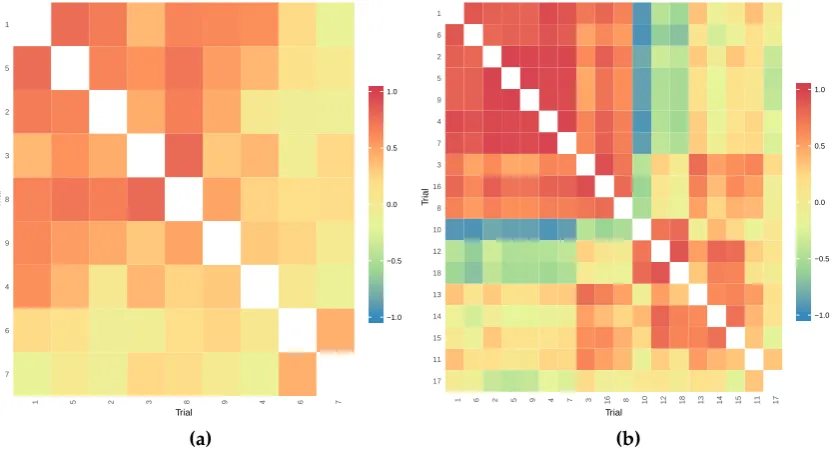
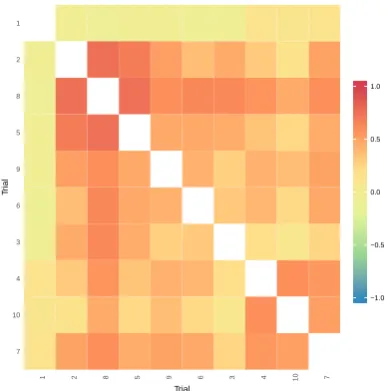
1.1 Flowchart showing the evolution of models used to analyse multi-environment trial data and how they relate to each other. . . 10 2.1 Heatmap showing the genetic correlations between trials from the

analysis of the (a) mungbean and (b) Desi chickpea data sets . . . . 29 2.2 Heatmap showing the genetic correlations between trials from the

analysis of the (a) Kabuli chickpea and (b) wheat data sets . . . 29 2.3 Flowchart demonstrating how the 40 data generation models were

formed for the simulation study. . . 34 2.4 Heatmap showing the genetic correlations between trials from the

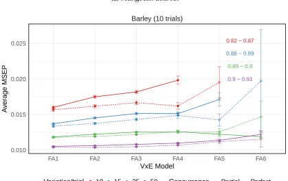
barley data set from Kellyet al. (2007). . . 36 3.1 Average mean square error of prediction (MSEP) for the FA models

from 500 simulations for the data generation models from the (a) mungbean and (b) barley variance-covariance structures . . . 41 3.2 Average mean square error of prediction (MSEP) for the FA models

from 500 simulations for the data generation models from the (a) Desi chickpea and (b) Kabuli chickpea variance-covariance structures 42 3.3 Average mean square error of prediction (MSEP) for the FA models

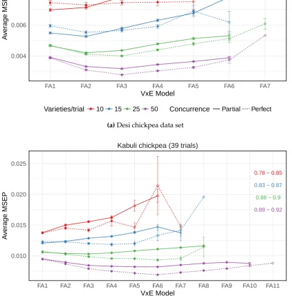
from 500 simulations for the data generation model from the wheat variance-covariance structures . . . 43 3.4 Average mean square error of prediction (MSEP) from 500

simu-lations for the data generation models from the (a) mungbean and (b) barley variance-covariance structures . . . 46 3.5 Average mean square error of prediction (MSEP) from 500

simu-lations for the data generation models from the (a) Desi chickpea and (b) Kabuli chickpea variance-covariance structures . . . 47 3.6 Average mean square error of prediction (MSEP) from 500

(16)

(17)

C

hapter

1

Literature review and introduction

Crop breeding programs conduct large numbers of field trials spanning multiple years and locations with the aim of breeding, selecting, and subsequently releas-ing crop varieties which outperform those currently available. These groups of trials are known as multi-environment trials (MET), where the term environment refers to year-location combinations. The aim of these trials is to investigate the performance of crop varieties in many environments in order to determine those which perform well across a range of environments and those which excel in specific environments (Smith et al., 2001). These trials form the foundation of crop breeding programs in Australia and many other countries and are the basis for which a crop variety may be deemed suitable for commercial release (Smith et al.,2005;Welhamet al.,2010). A variety is of the form below subspecies, having characteristics distinct from other varieties but able to be freely crossed with them.

Although the structure may differ slightly between countries, crop breeding programs typically contain multiple stages with the best varieties selected at each stage, so that the number of varieties tested decrease as the stages progress. The main focus of these breeding programs tends to be grain yield, although, many other traits may also be of interest and the concepts that will be discussed can easily be applied to other normally distributed traits. The early stages of the program consider early-generation material and large numbers of new breeding lines (usually greater than 500) are grown in a small number of field trials (usu-ally less than three), while in the final stages small numbers of elite breeding lines (usually less than 40) are grown in a large number of field trials spanning the country and consequently capturing a range of geographical locations and growing seasons (Smith et al., 2005). Due to the differences in the structure of the MET data originating from the early or late stages of the breeding programs, different considerations must be made for the analysis in each case.

1.1

Early methods for the analysis of MET data

(18)

by environment (VxE) effects, which describe the yield performance of different varieties across multiple environments. The aim is to determine whether the ob-served differences in yield are due to variety (genetic) differences, environment differences, or the interaction between variety and environment. Typically a two-stage method of analysis has been used which involves estimating the mean yield for each variety at individual trials and then combining the means from each trial to form the data for the second stage of the analysis (Smithet al.,2005). The second stage has been subject to a large range of statistical methods, with statisticians constantly attempting to better investigate the VxE interaction. Kempton(1984) discusses the classical analysis of variance (ANOVA) approach which fitted vari-ety and environment main effects along with a VxE interaction effect, partitioning the sum of squares into components accounting for varieties, environments, and the VxE interaction to gain insight into the variation in varietal response across different environments. However, this traditional approach fails to provide sub-stantial insight into the VxE interaction and in addition is difficult to interpret when there are large numbers of varieties and/or environments. Kempton(1984) mentions a number of methods that build on the traditional approach (ANOVA) with the aim of simplifying interpretation and deepening insight into the nature of the response of varieties across environments. These methods include further partitioning of the sum of squares through the classification of groups; regression analysis; principal components analysis; and the biplot technique.

Finlay & Wilkinson (1963) were some of the first authors to argue that the traditional ANOVA methods failed to adequately describe the VxE pattern and consequently proposed a linear regression method to compare the performance of varieties grown across a range of environments. The mean yield for each trial was used as an environmental index providing an evaluation of the environment. A linear regression was performed for each variety of individual yields on these environmental indices for each trial and the resulting regression coefficients used to categorise the sensitivity of a variety to environmental change. The regression coefficient along with the mean yield of a variety across environments provided an indication of a variety’s phenotypic stability and adaptability; for example a variety with a small regression coefficient and high mean yield should yield con-sistently well in all environments, meaning that it is phenotypically stable and well adapted to all environments. This method has been shown to be informative and is useful for summarising the VxE effects when the VxE effects have a strong linear association with the environmental index, however, this linear relationship may not always hold (Bythet al.,1976).

(19)

To address what they saw as the inadequacies of the regression method pro-posed byFinlay & Wilkinson(1963),Bythet al.(1976) proposed a two-way pattern analysis using numerical classification as an alternative option for investigating the VxE interaction. Pattern analysis had the advantage of not being dependent on the strength of the linear association between the VxE effects and an environ-mental index. Environments and varieties were each separately classified into 10 groups based on similarities in yield performance using the methods described byMungomeryet al.(1974). This resulted in reducing the size of the data matrix by 97 per cent but resulted in a loss of only 18 per cent of the total variation available in the full data set. Although this method summarised the data and meaning could be conveyed onto the groups in the example used byByth et al. (1976), generally these groups are arbitrary and difficult to interpret biologically, conveying little information regarding the VxE pattern (Kempton,1984).

Principal components analysis (PCA) has also been used to summarise the VxE effects. PCA is a popular multivariate technique producing linear com-binations (components) of the variables which describe variation in the data. The components are uncorrelated and are ordered such that the first component explains the largest proportion of variance in the original data, the second com-ponent explains the second largest proportion of variance and so on. Ideally the majority of the variation in the data could be described using only a small number of components, increasing the ease of interpretation. Gabriel(1971) proposed the biplot technique which provides a method to represent graphically the response of a variety across different environments. The biplot has the advantage that the expected response of a variety in a particular environment can be determined through visual inspection of the biplot. However, this method is most useful when a high proportion of the variation in the VxE effects can be explained by only one or two components, allowing the majority of the variation to be de-scribed in two dimensions, or a single biplot, as opposed to needing to interpret multiple biplots.

(20)

by the requirement of balanced data in which every variety is grown at every environment, something that is frequently not the case within breeding programs.

1.2

Linear Mixed Models

In the approaches that have been discussed variety and environment main effects and VxE interaction effects were all treated as fixed effects. When there is only interest in the treatments considered in the experiment, the effects are called fixed effects, however, when a factor in an experiment is considered to be a random sample from a population and the specific levels of the factor are of no interest, such as the effects of individual mice in an experiment, the effects are called ran-dom effects (Searle, 1997). A model that contains only fixed effects, aside from the error term which is always random, is known as a linear model, or fixed effects model. Similarly when all the effects in a model are random effects, the model is known as a random effects model and models which contain both fixed and random effects are known as mixed models. Random effects are assumed to follow a Gaussian distribution with mean zero and constant variance. The linear mixed model (LMM) is an extension of the linear model, allowing for correlated error terms and additional random components. The three advantages of the LMM compared with linear models identified by Smith et al. (2005) for MET data are the ease with which unbalanced data is handled; the potential to model within-experiment error variation more realistically; and the ability to assume some effects to be random rather than fixed. These advantages make these mod-els very flexible and underline why they have been embraced in the analysis of MET data.

In LMMs fixed effects are estimated using best linear unbiased estimation (BLUE) and random effects are estimated using best linear unbiased prediction (BLUP). There is a convention of “estimating” fixed effects and “predicting” ran-dom effects; however,Robinson(1991) states that “BLUP is a predictor only in the same way as most estimates are predictors”. In general the variance parameters necessary for the estimation of the fixed and random effects are unknown and are estimated through restricted maximum likelihood (REML,Patterson & Thomp-son 1971). Consequently the fixed and random effects are estimated as empirical BLUEs (E-BLUEs) and empirical BLUPs (E-BLUPs) respectively, as they are based on estimated, rather than known, variance parameters.

The estimation method of REML consists of maximising the likelihood of a set of selected error contrasts, which is achieved using a system of score equations that are solved iteratively.Patterson & Thompson(1971) utilised a Fisher scoring

(21)

algorithm, however, less computer intensive methods have been derived, such as first and second order derivative free methods which employ sparse matrix methods. The average information (AI) algorithm is a second order scheme pro-posed byGilmouret al.(1995), who showed it to be computationally convenient and efficient in the estimation of variance components when using REML. The AI algorithm is a modified Fisher scoring algorithm which uses an approximate average of the observed and expected information matrices rather than the ex-pected information matrix. It is especially powerful for large data sets with complex variance models (Smithet al.,2001).

Like early approaches to the analysis of MET data, early LMM applications tended to use a two-stage approach in which variety means were obtained from individual trial analyses in the first stage and then combined in an overall anal-ysis in the second stage, which can be either weighted or unweighted. However, LMMs are not restricted to a two-stage approach, and allow individual plot data from multiple trials to be analysed in a single analysis, known as a one-stage analysis. Within this one-stage analysis, a LMM approach also allows for fitting separate covariance structures for the residual effects at each trial, where residual effects refer to all effects peripheral to the VxE effects (Smithet al.,2001). Exam-ples of these include experimental design terms or terms to model field trend within a trial (see for exampleGilmouret al.(1997)).

(22)

There is some criticism of spatial models in that the estimated treatment effects rely solely on the chosen model. The advantages of spatial models are thought to outweigh the disadvantages; however, an approach that merges the randomisation and model based approaches is considered to be more robust (Smithet al.,2005). Using this merged approach the randomisation model is used as the base model and spatial models are used to explain remaining variation. When these hybrid models are applied to the analysis of MET data, they offer superior fits to the data compared to simple randomised complete block models which assume common block variance and plot variance for all trials and have rarely been found to provide good fits to Australian data (Smithet al.,2005).

1.3

Models for the VxE e

ff

ects in a LMM

Pattersonet al. (1977) were among the first to analyse MET data using a LMM, with such models becoming increasingly popular in the last three decades. Most early models included the VxE interaction effect as a random effect, and each of the variety and environment main effects as either fixed or random effects (Smith et al., 2005). Each of these random effects were assumed to follow a Gaussian distribution with mean zero and constant variance. These assumptions were somewhat limiting, assuming that environments had constant genetic variance, pairs of environments had constant genetic covariance, and environments had constant error variance. These assumptions have been acknowledged as ques-tionable by a number of authors (including Patterson & Silvey 1980; Patterson & Nabugoomu 1992;Culliset al. 1998) and consequently more complex models were proposed. However, with this added complexity comes added difficulty in fitting such models as more parameters must be estimated.

More complex mixed models made allowances for some heterogeneity of ge-netic variance between environments. Gogel et al.(1995) andNabugoomuet al. (1999) proposed a regression approach similar to the method popularised by Finlay & Wilkinson(1963), but in a mixed model setting. In these models envi-ronment means provide a quantitative grading of the envienvi-ronment and can be used as a surrogate for potentially complex environmental variables. However, it is important to note that environment means must be estimated from the data and are consequently subject to error.

Piephoet al.(1998) proposed an alternate regression based approach to explore the VxE interactions. This method modelled variety performance using covariate information on environments, such as average rainfall and soil type, rather than environment means. Piephoet al.(1998) utilised a separable variance matrix for

(23)

the VxE interaction effects which allowed for correlations between varieties. The advantage of this method over the regression method which uses environment means is that for suitable covariates (eg. rainfall or soil type), predictions of varietal performance to special environmental conditions can be generated when information on the response of a variety to environmental conditions is available.

The regression approaches proposed byGogelet al.(1995),Nabugoomuet al. (1999), andPiephoet al.(1998) have the advantage over the method popularised byFinlay & Wilkinson(1963) of being utilised in a mixed model setting. This al-lows unbalanced data to be analysed and complex covariance models to be used. However, like theFinlay & Wilkinson(1963) approach, these regression methods have the significant disadvantage of often explaining only a small proportion of the VxE interaction (Smithet al.,2005).

The multiplicative models proposed byPiepho(1997) andSmithet al. (2001) can be regarded as a random effects analogue of AMMI. The multiplicative model applied to the VxE interaction effects was that associated with the multivariate technique of factor analysis. The variance structure for the VxE effects is known as the factor analytic (FA) structure of orderk. When the FA model is applied to the variety effects in each environment, as in the case ofSmithet al.(2001), they are decomposed into a regression ofkhypothetical factors on variety scores along with a lack of fit term for the model. The FA model for the VxE effects differs from traditional random regression problems in that both the coefficients and covariates must be estimated from the data, where the covariates are known as variety scores and the coefficients as environmental loadings. This FA model re-sults in heterogeneity of variety variance and covariance between environments, rather than constraining variance and covariance parameters to be equal as in earlier models. Consequently this model allows more realistic modelling of the VxE effects. Piepho (1997) proposed a similar model, however, with random environment effects rather than random variety effects, resulting in heterogene-ity of VxE variance and covariance between varieties. The model proposed by Smithet al.(2001) also differed from that proposed byPiepho(1997) in that they allowed a separate variance to be estimated for each environment in the lack of fit component of the FA model, known as specific variances.

(24)

predict the true variety effects and assuming that the estimates of the variance parameters are sufficiently precise, this also holds true for E-BLUPs. If the aim of the analysis is selection of the best varieties, E-BLUPs are most appropriate and varieties should be treated as random because the rankings of the estimated variety effects need to be as precise as possible with regard to the rankings of the true variety effects (Smithet al.,2005). However, if the aim is to estimate the differences between specific variety effects as precisely as possible variety effects should be treated as fixed because the use of E-BLUPs are inappropriate given that the BLUP of a specific difference is biased. The aim of breeding trials is to select superior varieties and as a result the use of random variety effects is appropriate. Smith et al. (2005) highlight that with balanced data and orthogonal analyses, models with fixed or random variety effects would result in identical rankings of these effects; however, these authors prefer the use of random variety effects due to their advantage of more realistic estimates of genetic gain, as such esti-mates tend to be overly optimistic due to selection bias (Patterson & Silvey,1980).

The flexibility of the FA model means that for large data sets a substantial number of variance parameters must be estimated. Despite its power, the AI algorithm falls short for FA models when one or more of the estimates of specific variances tend towards zero, resulting in the variance matrix for VxE effects being of less than full rank (termed reduced rank). As such a modified version of the AI algorithm was necessary. Thompson et al. (2003) presented a sparse imple-mentation of the AI algorithm for REML estimation of FA variance parameters for the reduced rank case. In addition to allowing for the fitting of reduced rank variance models, this implementation also has the advantage of faster conver-gence compared to the algorithm proposed bySmithet al.(2001) when fitting FA models due to the use of sparse matrices in the estimation process.

Although a one-stage analysis is typically used in Australia for the analysis of early-generation MET analyses and short-term MET analyses, an approximate two-stage approach is used when analysing long-term METs in Australia, along with replicated late-stage MET data in the UK (Welhamet al.,2010). Welhamet al. (2010) suggest that this is due to individual plot data traditionally being difficult to find due to it not being stored electronically, along with the computational dif-ficulties involved with a single-stage analysis when complex variance models are used. Although the more efficient one-stage approach has been recommended (Smithet al.,2005),Welhamet al.(2010) formally evaluated the one- and two-stage (both weighted and unweighted) approaches using a simulation study. The study considered six statistical models and three different analysis methods, with the

(25)

three analysis methods consisting of a single-stage analysis, a weighted two-stage analysis, and an unweighted two-stage analysis. The MET data sets used in the study were simulated from the characteristics and estimated parameters from an Australian wheat breeding program and a set of UK recommended list wheat trials in order to be representative of actual data. The mean square error of pre-diction and relative genetic gain were used to assess the accuracy of the variety predictions in each environment compared to the effects used to simulate the data.

Welham et al. (2010) found that a one-stage approach resulted in the most accurate prediction of variety performance for a range of models. They also found that the unweighted two-stage analysis resulted in a loss of important information regarding estimates of variety performance, however, the weighted two-stage analysis provided an adequate approximation to the single-stage anal-ysis, and may be used for large data sets when the one-stage analysis becomes computationally impractical (Welhamet al.,2010). The range of models used to analyse MET data are summarised in Figure 1.1, with distinctions for one- and two-stage analyses. This figure demonstrates how the models evolved and how they relate to each.

1.4

Extensions to the model for VxE e

ff

ects

(26)

10

ANOVA _LMM

Data Reduction

Regression

• Finlay & Wilkinson (1963)

LMM

• Patterson & Thompson (1971)

• Patterson et al.(1977)

• Patterson & Silvey (1980)

• Patterson & Nabugoomu (1992)

Group Classification

• Mungomeryet al.(1974)

• Bythet al.(1976)

PCA

Biplot technique

• Gabriel (1971) AMMI

• Kempton (1984)

• Gauch (1992) _{LMM regression}

• Gogelet al.(1995)

• Piephoet al.(1998)

• Nabugoomuet al.(1999)

Single stage MET Analyses Spatial models

• Cullis & Gleeson (1991)

• Gilmour et al.(1997)

• Culliset al.(1998)

FA models

• Piepho (1997)

• Smith et al. (2001)

Two-stage analysis

One-stage analysis

Stage one

[image:26.595.54.777.66.458.2]

Stage two

(27)

varieties are highly inbred, non-additive effects will reflect epistatic effects (in-teractions between genes within an individual) because inbreeding will largely eliminate dominance.

Although the inclusion of pedigree information has been shown to result in superior model fit (Oakey et al., 2007; Beeck et al., 2010), the elements of the relationship matrix are approximate to true relatedness based on an average proportion of genes in common, and in reality can be quite different to what is expected (Borgognoneet al.,2016). The benefits of including pedigree information in the analysis are seen to outweigh the limitations resulting from the approx-imations necessary in forming this matrix, however, an alternative relationship matrix can be derived from the molecular marker information. Borgognoneet al. (2016) proposed using an FA model for the analysis of MET data with the ge-nomic relationship matrix rather than the additive relationship matrix to model the relationship between varieties. The form of the genomic relationship matrix still allowed for the partitioning of genetic effects into additive genetic effects and non-additive genetic effects and resulted in lower average prediction error variance of genetic effects (Borgognoneet al.,2016).

The use of FA models in the analysis of MET data also allows for investigation into the varied nature of the VxE effects, exploring patterns and irregularities in the data, along with simplifying the results and interpretation. Culliset al.(2010) proposed a number of statistical tools to explore the VxE interactions, including heatmaps which display visually the genetic correlations between environments and clustering methods which group environments in which varieties perform similarly in terms of rank position. These tools can simplify and aid in the inter-pretation of what can be large numbers of VxE effects. The use of an FA model allows for investigation into a variety’s environmental stability for the environ-ments considered in the data, through the regression form of the VxE effects. However, this regression is inherent within the FA model; no post-processing is necessary (Smithet al.,2015).

(28)

of barley varieties which maintain large, stable grain size across a range of envi-ronments. In a different approach,Christopheret al.(2014) used an FA structure to model variety effects for different traits, estimating the genetic correlations between yield, stay-green traits and normalised difference vegetative index mea-surements, where these traits were used as environments.

Stefanova & Buirchell(2010) analysed 39 trials of 25 historical lupin varieties using an FA model for the VxE effects. They found that the variety scores for the first two factors of the regression structure of the FA model were representa-tive of genetic gain and stability of varieties. This analysis allowed the authors to identify the varieties which were adapted to low, medium and high rainfall zones and to assess genetic gain over a 31 year period.

Thompsonet al. (2011) used an FA model to analyse MET data sets measur-ing the densities of root-lesion nematodesPratylenchus thorneiand Pratylenchus neglectus in chickpea. The aim of this experiment was to investigate the sus-ceptibility of Australian and international chickpea varieties to these nematodes, allowing for more informed decisions in planning rotations in fields infested with eitherP. thorneiorP. neglectus. Roddaet al.(2016) also modelledP. thorneidensity in chickpeas across a number of trials undertaken in the glasshouse and the field using an FA model. These models enabled the authors to determine that the relative differences in resistance toP. thorneiidentified were highly heritable and also that the genetic correlation between trials in the glasshouse and field were high, meaning that resistance toP. thorneiin chickpea can be effectively selected

in a limited set of environments, saving in labour and resources.

Kellyet al.(2007) investigated the accuracy of FA models for trials with large numbers of varieties. FA models were compared with LMMs fitting three models for the VxE effects. These models were a diagonal model, in which the genetic covariance between all pairs of environments is zero, a uniform model, which assumes constant genetic variance and constant genetic covariance across envi-ronments, and an unstructured model, which allows a large degree of flexibility in the genetic variance and covariance parameters across environments. The FA models were shown to generally be the model of best fit for a range of data sets taken from early-generation trials in a breeding program. Additionally the su-periority of FA models in selection of varieties was shown through a simulation study. The number of varieties considered in this study were 500, 200, and 80, which are representative of the number of varieties per trial included in the early stages of a breeding program.

(29)

1.5

Research aims

The number of varieties per trial considered in the late stages of a breeding program are substantially smaller than in the earlier stages and the accuracy of FA models for small numbers of varieties in each trial has not been properly investigated. This prompts the question, does an FA model provide the best estimate of the VxE interaction effects for METs with smaller numbers of varieties? The aims of this project are

1. to determine whether the adequacy of an FA variance structure changes as the number of crop varieties within a trial decreases;

2. to investigate the implications the underlying VxE variance structure has on the accuracy of the FA model; and

(30)

(31)

C

hapter

2

Methods

In the first section of this chapter, Section2.1, the statistical theory behind linear mixed models will be discussed. This includes the derivation of the residual likelihood and REML score equations which are used to estimate variance pa-rameters, along with the estimation of fixed and random effects. Following this, in Section2.2the selection and analysis of the primary data sets used to provide parameters for a simulation study will be detailed. The final section of this chap-ter, Section2.3, explains the simulation study that was conducted to investigate the aims of this project.

2.1

Statistical method theory

2.1.1 Linear mixed models

Consider a series ofttrials (synonymous with environments) in whichmvarieties have been grown. Ifnj are the number of plots in the jth trial,n =

Pt

j=1nj is the

total number of plots. A general linear mixed model for the n× _{1 vector of}

individual plot yields,y, ordered as plots within trials, can be written as

y=1nµ+Xeτe+Xpτp+Zgug+Zpup+e (2.1) whereµis the overall mean, τe is at×1 vector of fixed trial effects with design matrix Xe, and ug is a mt × 1 vector of random variety effects for each trial (ordered as varieties within trials) with design matrixZg. The vectorτpcontains trial specific fixed effects with corresponding design matrixXpand the vectorup contains trial specific random effects with corresponding design matrixZp. The

n×_{1 vector}_econtains residual effects. The random effects are assumed to follow

a Gaussian distribution with mean zero and variance matrix

var            ug up e            =           

Gg 0 0

0 Gp 0

0 0 R

           .

(32)

variance of the VxE effects can be partitioned into variance due to environments and variance due to varieties such that

Gg =Ge⊗Gv,

where Ge and Gv are the t×t and m×m symmetric matrices for the variance for environments and varieties respectively. A common assumption is that the variety effects are independent (Smithet al.,2001) such thatGv =Im.

The trial specific effects and the residual effects are assumed to be indepen-dent for each trial such thatGp = diag(Gpj) andR = diag(Rj), whereGpj is the

variance matrix for the trial specific random effects at the jth trial andRj is the residual variance matrix for trial j. The simplest formRj can take isRj = σ2_jInj

which assumes plot residual effects are independent. However,Smithet al.(2001) utilised the approach ofGilmouret al. (1997) incorporating a spatial correlation matrix, such thatRj =σ2_jΣcj ⊗Σrj, whereΣcj and Σrj are the correlation matrices

for columns and rows respectively, andσ2

j is the associated variance.

The traditional mixed model includes a variety main effect and a VxE inter-action effect (Pattersonet al.,1977), such that

ug =(1t⊗Im)uv+uge,

with these random effects following a Gaussian distribution with mean zero and variance matrix var       uv uge      =       σ2

gIm 0

0 σ2ge(It⊗Im)      ,

where σ2

g and σ2ge are the estimated variance components for variety and the

interaction between variety and environment respectively. This leads to

var(ug)=var((1t⊗Im)uv+uge) =(1t⊗Im)var(uv)(1t⊗Im)

0

+var(uge) =(1t⊗Im)σ2gIm(1

0

t⊗I

0

m)+σ2ge(It⊗Im) =σ2

g(1t⊗Im)(1

0

t⊗I

0

m)+σ2ge(It⊗Im) =σ2

g(1t1

0

t)⊗(ImIm)+σ2ge(It⊗Im)

=(σ2gJt+σ2geIt)⊗Im (2.2) ≡_G_e⊗_I_m,

(33)

resulting in common genetic variance,σ2

g+σ2ge, for all environments and a

com-mon genetic covariance, σ2

g, between pairs of environments. This form of Ge is known as a uniform variance structure.

An alternative, and generally preliminary, model for Ge is an independent model, also known as a diagonal (DIAG) variance model. This model allows for heterogeneity of genetic variance for different environments and assumes zero covariance between pairs of environments, such that

var(ug)=                  σ2 g1 0 σ2

g2

... ...

0 0 · · · σ2

gt                 

⊗_I_m _(2.3)

≡_G_e⊗_I_m,

whereσ2

gj is the genetic variance for the jth trial.

The most general form of the genetic variance matrix,Ge, is an unstructured matrix, which containst(t+1)/2 parameters and can be expressed as

var(ug)=                  σ2 g1

σg12 σ 2

g2

... ...

σg1t σg2t · · · σ

2 gt                 

⊗_I_m _(2.4)

≡_G_e⊗_I_m,

whereσ2

gj is the genetic variance at the jth trial, andσgi j is the genetic covariance

between trialsiand j. Although this model has desirable attributes, it is difficult

to estimate from a computational perspective. Furthermore it may be inefficient or unstable for even moderately large numbers of environments (Smith et al., 2001), andSmithet al.(2005) suggest this is also true for large numbers of vari-eties.

(34)

kcan be written as

ug =(Λ⊗Im)f +δ,

whereΛis at×_k_{matrix of environment loadings,} _f _{is a}_mk×_{1 vector of variety}

scores, andδis amt×_{1 vector of residuals for the VxE model. The joint distribution}

of f and δ are assumed to follow a Gaussian distribution with mean zero and variance matrix var       f δ      =      

Ik⊗Im 0

0 Ψ⊗_I_m      ,

whereΨis a diagonalt×_t_{matrix of elements commonly referred to as specific}

variances. The variance matrix of the variety scores is an identity matrix which means that the scores have a constant variance of 1 and are all independent of each other. The variance of the VxE effects, ug, under this model results in heterogeneity of genetic variance for different environments and heterogeneity of genetic covariance between pairs of environments.

var(ug)=var((Λ⊗Im)f +δ)

=(Λ⊗_I_m₎₍_I_k⊗_I_m₎₍Λ⊗_I_m₎0+Ψ⊗_I_m

=(Λ⊗_I_m₎_I_km₍Λ0⊗_I0

m)+Ψ⊗Im =(ΛΛ0)⊗_I_m+Ψ⊗_I_m

=(ΛΛ0+Ψ)⊗_I_m _(2.5)

≡_Ge⊗_I_m,

where the genetic variance for each trial is given by the diagonal elements of

ΛΛ0₊_Ψ_{and the genetic covariance between pairs of trials are the off-diagonal}

elements ofΛΛ0

.

2.1.2 Estimation

The variance parameters of the linear mixed model are estimated using REML and the fixed and random effects are estimated as e-BLUEs and e-BLUPs respec-tively as discussed in Section 1.2. The following section derives the residual likelihood and the REML score equations, along with the estimates of the fixed and random effects.

The model in Equation2.1can be rewritten using the general form for a linear mixed model

y=Xτ+Zu+e, (2.6)

whereτ =µ,τ0 e,τ

0 p

0

is a vector of fixed effects with design matrixX =h1nXeXp i

andu=u0 g,u

0 p

0

is a vector of random effects with design matrixZ=hZg Zpi. The

(35)

random effects are assumed to follow a Gaussian distribution, with mean zero and variance matrix

var       u e      =       G 0 0 R      ,

where G = diag(Ge,Gp). The vectors of variance parameters associated with the random and residual effects areγ =

γ0 e,γ

0 p

0

and φ respectively, such that

G= G(γ), R =R(φ). The distribution of yis consequently Gaussian with mean

Xτand variance matrixH =R+ZGZ0

.

Residual maximum likelihood

Verbyla(1990) provided a useful derivation of the likelihood function in which it is partitioned into two independent parts, relating to the treatment contrasts and the residual contrasts. Verbyla(1990) utilised a matrix,L =h L1 L2

i

, such that

L₁n×p and L₂n×(n−p) satisfy the conditions L0

1X = IP and L

0

2X = 0. L is then used to transformytoL0ysuch that

L0y=       L0 1 L0 2      y=

      y1 y2      .

The mean ofL0

yis found by

E(L0y)=L0E(y)=

      L0 1 L0 2      Xτ =

      L0

1Xτ

L0

2Xτ

     =      

Ipτ 0      =       τ 0      .

The variance ofL0

yis found by

var(L0y)=L0var(y)(L0)0 =L0HL=      

L0₁ L0 2      H h

L1 L2

i =       L0 1H L0 2H       h

L1 L2

i =       L0

1HL1 L

0

1HL2

L0

2HL1 L

0

2HL2

     .

Consequently the distribution ofL0 yis       y1 y2       ∼_N             τ 0      ,      

L0₁HL1 L

0

1HL2

L0

2HL1 L

0

2HL2

          

. (2.7)

The likelihood ofL0

ycan be expressed as the product of the conditional likelihood of y1 given y2 and the marginal likelihood of y2. The log-likelihood of these distributions can be expressed similarly such that

lF τ, κ;L 0

y =

(36)

Using the standard results in AppendixA.1and the work ofVerbyla(1990) in AppendixA.2the mean and variance of y1|y2can be found

E(y1|y2)=τ+L

0

1HL2(L

0

2HL2)

−₁

y2−0 =τ+L0₁HL2(L0₂HL2)−1y2

var(y1|y2)=L

0

1HL1−L

0

1HL2(L

0

2HL2)

−₁ L0₂HL1 =h

L0₁H−_HL₂₍_L0

2HL2)

−₁

L0₂HL1

i

=h

L0₁X(X0H−1X)−1X0L1

i

=h Ip(X

0

H−1X)−1I_p0i

=(X0H−1X)−1.

The conditional distribution ofy1|y2 is consequently

y1|y2 ∼N

τ+L0₁HL2(L₂0HL2)−1y2,(X

0

H−1X)−1

and its corresponding log-likelihood function (excluding constants) is

lT =−

1

2log|(X

0

H−1X)−1| − 1

2

y1−τ−L

0

1HL2(L

0

2HL2)

−₁ y2

₀

(X0H−1X)y1−τ−L

0

1HL2(L

0

2HL2)

−₁ y2

=− 1

2

log|₍_X0_H−1_X₎−1|+

L0₁y−τ−_L0

1HL2(L

0

2HL2)

−₁ L0₂y0

(X0H−1X)L0₁y−τ−_L0

1HL2(L

0

2HL2)

−₁ L0₂y

.

The marginal distribution ofy2is

y2 ∼N 0,L

0

2HL2

and its associated log-likelihood (excluding constants) is

lR=−

1 2

log|_L0

2HL2|+y

0 L2 L

0

2HL2

−₁ L0

2y

.

Given that the likelihood ofL0

ycan be expressed as the product of the condi-tional likelihood ofy1giveny2and the marginal likelihood of y2, its determinant

(37)

can be similarly partitioned using the determinant properties in AppendixB.3.

log|_L0_HL|=_log|_L0

2HL2|+log|(X

0

H−1X)−1|

log|_L0_L|+_log|_H|=_log|_L0

2HL2| −log|X

0 H−1X|

log|_L0

2HL2|=log|L

0

L|+_log|_H|+_log|_X0_H−1_X|

The log-likelihood of the marginal distribution ofy2, excluding constants, can be rewritten as

lR =−

1 2

log|_H|+_log|_X0_H−1_X|+_y0_L₂ _L0

2HL2

−1 L0₂y

=−1

2

log|_H|+_log|_X0_H−1_X|+ _y0_Py,

where P = L2

L0

2HL2

−1 L0

2. This residual log-likelihood is used to estimate the variance parameters.

The REML solutions forκ=γ0,φ0

0

are obtained from the solution of the set of equations

UR(κi)= ∂lR ∂κi =

0,

known as score equations, fori = 1, . . . ,nk, where nk is the number of variance

parameters inκ.

The score equation forκiis given by

UR(κi)=−

1 2

∂

∂κi

log|_H|+ ∂ ∂κi

log|_X0_H−1_X|+ ∂

∂κi

y0Py

.

Using the derivative results in SectionB.6,

∂ ∂κi

log|_H|=

trH−1Hi˙ ,

where ˙Hi = ∂H_∂κ_i, and

∂ ∂κi

log|_X0_H−1_X|=tr _X0_H−1_X−1 ∂

∂κi

X0H−1X !

=tr

X0H−1X −₁

X0 ∂ ∂κi

H−1X !

=tr

X0H−1X−1X0−H−1HiH˙ −1X

=−_tr

X0H−1X −₁

X0H−1HiH˙ −1X

(38)

Using the results in AppendixA.3,

∂ ∂κi

y0Py= y0 ∂

∂κi

(P)y

=y0PHiPy˙ .

Combining these results, the score equation forκi is

UR(κi)=−

1 2

trH−1Hi˙ −_tr

X0H−1X−1X0H−1HiH˙ −1X

−_y0_P_HiPy˙

=− 1

2

tr

H−1Hi˙ −_H−1_X_X0_H−1_X −₁

X0H−1Hi˙

−_y0_P_HiPy˙

=− 1

2

tr

H−1−_H−1_X_X0_H−1_X −₁

X0H−1

˙

Hi

−_y0_P_HiPy˙

=− 1

2

trPHi˙ −_y0_P_HiPy˙

. (2.9)

Generally solving the system of equationsUR(κ)=0 requires an iterative method

(Smithet al.,2001). One such method is the average information (AI) algorithm (Gilmouret al., 1995). The AI algorithm is a modified Fisher scoring algorithm which uses an approximate average of the observed and expected information matrix rather than the expected information matrix. As shown in Smith et al. (2005), given an estimate ofκ=κ(m)_{, it can be updated as}

κ(m+1) ₌_κ(m)₊h_I(m)i−1_U

R(κ(m)),

whereI(m)_{is the average information matrix,}_I_{, for iteration (}_m_{) given by}

I= 1

2Q

0 PQ

and the columns ofQare working variables associated withκgiven by

qκi =HiPy˙ .

Mixed model equations

Estimates of the fixed and random effects, τandu, can be found by maximising a function derived from the joint distribution ofyandu, such that

(39)

The log-density function for the joint distribution of yanduis given by

log fY(y|u)+log fU(u).

The distribution ofuis given by

u∼_{N (0},_G₎

and its associated log-density function is

logfu =−

1 2

log|_G|+_u0_G−1_u.

Using the findings in AppendixA.1the mean and variance of y|_u_{can be found}

E(y|_u₎=_Xτ+_ZGG−1₍_u−₀₎

=Xτ+Zu

var(y|_u₎=_H−_ZGG−1_GZ0

=H−_ZGZ0

=R.

The conditional distribution ofy|_u_{is consequently}

y|_u∼_{N (}_Xτ+_Zu,_R₎

and its associated log-density function is

logfY =−

1 2

log|_R|+₍_y−_Xτ−_Zu₎0_R−1₍_y−_Xτ−_Zu₎.

The log-density function for the joint distribution of yanduis given by

logfu+logfY =−

1 2

log|_G|+_u0_G−1_u

− 1

2

log|_R|+

(y−_Xτ−_Zu₎0_R−1₍_y−_Xτ−_Zu₎

. (2.10)

Differentiating Equation2.10with respect toτusing results in AppendixB.6 and equating to zero results in

(40)

X0R−1Xτˆ +X0R−1Zu˜ =X0R−1y, (2.11) where ˆτand ˜uare the estimates ofτandurespectively. Differentiating Equation

2.10with respect touusing results in AppendixB.6and equating to zero results in

2G−1u˜−₂_Z0_R−1₍_y−_Xτ_ˆ −_Z_u_˜₎=₀ G−1u˜−_Z0_R−1_y+_Z0_R−1_Xτ_ˆ +_Z0_R−1_Z_u_˜ =₀

Z0R−1Xτˆ+G−1+Z0R−1Zu˜ =Z0R−1y. (2.12) Equations2.11and2.12 are known as the mixed model equations and are more commonly expressed using matrix notation as

      X0

R−₁

X X0

R−₁ Z Z0

R−₁

X (G−₁₊ Z0

R−₁ Z)             ˆ τ ˜ u      =       X0

R−₁ y Z0

R−₁ y     

. (2.13)

Rearranging Equation2.12gives

˜

u=G−1+Z0R−1Z −₁

Z0R−1y−_Z0_R−1_Xτ_ˆ _(2.14)

and substituting Equation2.14into2.11gives

X0R−1Xτˆ +X0R−1ZG−1+Z0R−1Z−1Z0R−1y−_Z0_R−1_Xτ_ˆ=_X0_R−1_y X0R−₁

Xτˆ −_X0_R−1_Z_G−1+_Z0_R−1_Z −₁

Z0R−₁

Xτˆ =X0R−₁

y−_X0_R−1_Z_G−1+_Z0_R−1_Z −₁

Z0R−₁ y

X0

R−₁₋ R−₁

ZG−₁

+Z0

R−₁

Z−1Z0

R−₁

Xτˆ =X0

R−₁₋ R−₁

ZG−₁

+Z0

R−₁

Z−1Z0

R−₁ y.

Using the identity in Appendix B.4, this can be rewritten in terms of H−₁

, such that

X0H−1Xτˆ =X0H−1y

ˆ

τ=

X0H−1X−1X0H−1y. (2.15)

Substituting Equation2.15into2.14gives

˜

u=G−1+Z0R−1Z−1

Z0R−1y−_Z0_R−1_X_X0_H−1_X−1_X0_H−1_y

=

G−1+Z0R−1Z −₁

Z0R−1

I−_X_X0_H−1_X −₁

X0H−1

y

=

G−1+Z0R−1Z −₁

Z0R−1HPy

=h

G−_GZ0₍_R+_ZGZ0₎−1_ZGi_Z0_R−1_HPy

(41)

=GZ0hI−_H−1_ZGZ0i_R−1_HPy

=GZ0hI−_H−1₍_H−_R₎i_R−1_HPy

=GZ0hI−_I+_H−1_Ri_R−1_HPy

=GZ0H−1RR−1HPy

=GZ0Py. (2.16)

Utilising Equations 2.15 and 2.16, in conjunction with the score equations shown in Equation2.9, the fixed and random effects can be estimated. The VxE effects can be used to select the best performing varieties in each environment and the estimates of genetic variance and genetic covariance provide important information about the nature of the VxE effects and whether varieties perform similarly in certain environments. A practical example of the implementation of this process will be given in the following section.

2.2

Primary data sets and estimation of simulation parameters

Four primary data sets were selected and analysed to provide parameters to be used as the basis for a simulation study. Using these parameters 20 000 data sets were simulated to assess the performance of FA models when data sets contain trials with small to moderate numbers of varieties. The methods and results of this preliminary analysis are included in this section as they represent a necessary step towards the simulation of the data sets and the subsequent analysis of these simulated data sets, which is the focus of this research.

2.2.1 Selection of primary data sets

Four data sets originating from crop breeding programs were analysed, demon-strating the methods typically employed in the analysis of MET data. These data sets were chosen as they are representative of different crop types for late stage breeding programs in Australia. The selected data sets consist of data from the late stages of a wheat breeding program, two chickpea breeding programs (one considering Desi chickpeas and the other Kabuli chickpeas), and a mungbean breeding program. This section details the analysis of these data sets along with the results of these analyses.

(42)

unique varieties. The data sets differ in the level of varietal concurrence between trials. A measure of the average varietal concurrence for each data set is given by the number of unique trial-by-variety combinations present in the data, divided by the potential number of unique combinations given the number of trials and varieties. Both the Desi chickpea and mungbean data sets have an average of approximately 60% of varieties in common between trials, while the remaining two data sets have much lower concurrence with an average of 38% and 28% for wheat and Kabuli chickpea respectively. The poor concurrence for these two data sets is driven by the number of years considered. All of the data sets have nearly perfect concurrence between trials from the same year, however, a number of varieties are often removed from the program each year and replaced with new varieties. This results in increasingly poor concurrence as more years are consid-ered, and it is for this reason breeding programs tend to use a moving window of approximately five years for the analysis of multi-environment trial data. The analyses for all data sets were performed using yield as the dependent variable.

2.2.2 Analysis of primary data sets

The data sets were each analysed separately using standard analysis procedures for multi-environment trials. The yield data from each trial was initially analysed separately using a linear mixed model, equivalent to that shown in Equation2.1. The model fitted an overall mean and a random variety effect, along with any significant trial specific covariates (such harvesting problems or bird damage). Using the approach discussed in Section1.2(Smithet al.,2005), experimental de-sign terms were included as random effects and spatial variation was modelled following the procedure ofGilmouret al.(1997). The residual (plot) effects were modelled using a separable variance structure, with a first order autoregressive model used in both the row and column directions. Diagnostic tools were used to assess spatial variation in the field, with formal tests used to determine whether terms accounting for this spatial variation should be included in the model.

Table 2.1: Summary of data sets used as sources of parameter estimates for data simulation.

Data set Years Trials Varieties Varieties per trial Concurrence (%) Min Mean Max Overall Per year

Desi Chickpea 2 18 50 30 30 30 60 100

Kabuli Chickpea 6 39 223 51 63 85 28 99

Mungbean 2 9 78 25 52 73 66 100

Wheat 4 52 128 42 49 60 38 99

(43)

Following the single-trial analyses, trials were combined in a multi-environment trial (MET) analysis. Spatial and design terms along with residual effects were modelled separately for each trial, using the models found in the single-trial analysis. Initially the variety by environment (trial) effects were modelled in-dependently for each trial. This model was then extended to a factor analytic (FA) model of order 1. Higher order FA models were subsequently fitted to the VxE effects given they provided an improvement on the previous model and the inequality

k≤ 2t+1− √

8t+1

2 (2.17)

was satisfied, wherek is the order of FA model and tis the number of trials in the data. The Akaike information criterion (AIC) and log-likelihood ratio test were used to determine the order of the most parsimonious FA model within each data set, where all comparisons were made between nested models. Both of these are measures of goodness-of-fit, where smaller relative AIC values and a significant log-likelihood ratio test under a Chi-square distribution indicate a more parsimonious model. A summary of the models for each data set is shown in Table2.2. All analyses were undertaken using ASReml-R (Butleret al.,2009) in the R software environment (R Core Team,2016).

2.2.3 Analysis results of data sets

(44)

[image:44.595.111.428.167.557.2]

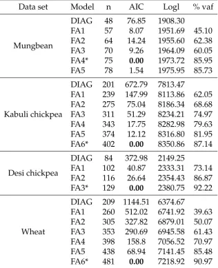
Table 2.2: Summary of models used to analyse selected data sets, showing the number of parameters estimated in the model (n), the Akaike information crite-rion (AIC), given here as the difference between the model and the model with the smallest AIC in each data set, the log-likelihood (Logl), and percent of genetic variance accounted for by the FA components in the model (% vaf).

Data set Model n AIC Logl % vaf

Mungbean

DIAG 48 76.85 1908.30

FA1 57 8.07 1951.69 45.10 FA2 64 14.24 1955.60 62.38 FA3 70 9.26 1964.09 60.05 FA4* 75 0.00 1973.72 85.95 FA5 78 1.54 1975.95 85.73

Kabuli chickpea

DIAG 201 672.79 7813.47

FA1 239 147.99 8113.86 62.05 FA2 275 75.04 8186.34 68.68 FA3 311 51.29 8234.21 74.97 FA4 343 17.75 8282.98 79.63 FA5 374 12.12 8316.80 81.95 FA6* 402 0.00 8350.86 87.14

Desi chickpea

DIAG 84 372.98 2149.25

FA1 102 40.87 2333.31 73.14 FA2 116 26.64 2354.43 86.87 FA3* 129 0.00 2380.75 92.22

Wheat

DIAG 209 1144.51 6374.67

FA1 260 512.02 6741.92 39.63 FA2 305 327.82 6879.01 50.07 FA3 353 290.69 6945.58 61.43 FA4 398 158.8 7056.52 70.97 FA5 438 68.94 7141.45 85.48 FA6* 481 0.00 7218.92 90.97

* Model which offered the best fit to the data according to a

log-likelihood ratio test.

variance than error variance. There were also two Desi chickpea trials that had much more (over 10 times) genetic variance than error variance. This preliminary analysis of these four data sets resulted in the parameters that formed the basis of the simulation study as discussed in the next section.

(45)

7 6 4 9 8 3 2 5 1

1 5 2 3 8 9 4 6 7

Tr