White Rose Research Online URL for this paper:
http://eprints.whiterose.ac.uk/80043/
Version: Published Version
Article:
Marra, WA, Parsons, DR, Kleinhans, MG et al. (2 more authors) (2014) Near-bed and
surface flow division patterns in experimental river bifurcations. Water Resources
Research, 50 (2). 1506 - 1530. ISSN 0043-1397
https://doi.org/10.1002/2013WR014215
[email protected]
https://eprints.whiterose.ac.uk/
Reuse
Unless indicated otherwise, fulltext items are protected by copyright with all rights reserved. The copyright
exception in section 29 of the Copyright, Designs and Patents Act 1988 allows the making of a single copy
solely for the purpose of non-commercial research or private study within the limits of fair dealing. The
publisher or other rights-holder may allow further reproduction and re-use of this version - refer to the White
Rose Research Online record for this item. Where records identify the publisher as the copyright holder,
users can verify any specific terms of use on the publisher’s website.
Takedown
If you consider content in White Rose Research Online to be in breach of UK law, please notify us by
RESEARCH ARTICLE
10.1002/2013WR014215
Near-bed and surface flow division patterns in
experimental river bifurcations
Wouter A. Marra1,2, Daniel R. Parsons2,3, Maarten G. Kleinhans1, Gareth M. Keevil2,
and Robert E. Thomas2,3
1Faculty of Geosciences, Universiteit Utrecht, Utrecht, Netherlands,2School of Earth and Environment, University of Leeds,
Leeds, UK,3Now at: Department of Geography Environment and Earth Sciences, University of Hull, Hull, UK
Abstract
Understanding channel bifurcation mechanics is of great importance for predicting and man-aging multichannel river processes and avulsion in distributary river deltas. To date, research on river chan-nel bifurcations has focused on factors determining the stability and evolution of bifurcations. It has recently been shown that, theoretically, the nonlinearity of the relation between sediment transport and flow discharge causes one of the two distributaries of a (slightly) asymmetrical bifurcation to grow and the other to shrink. The positive feedback introduced by this effect results in highly asymmetrical bifurcations. However, there is a lack of detailed insight into flow dynamics within river bifurcations, the consequent effect on bed load flux through bifurcating channels, and thus the impact on bifurcation stability over time. In this paper, three key parameters (discharge ratio, width-to-depth ratio, and bed roughness) were varied in order to examine the secondary flow field and its effect on flow partitioning, particularly near-bed and surface flow, at an experimental bifurcation. Discharge ratio was controlled by varying downstream water levels. Flow fields were quantified using both particle image velocimetry and ultrasonic Doppler velocity profiling. Results show that a bifurcation induces secondary flow cells upstream of the bifurcation. In the case of unequal discharge ratio, a strong increase in the secondary flow near the bed causes a larger volume of near-bed flow to enter the dominant channel compared to surface and depth-averaged flow. However, this effect diminishes with larger width-to-depth ratio and with increased bed roughness. The flow structure and division pattern will likely have a stabilizing effect on river channel bifurcations. The magnitude of this effect in relation to previously identified destabilizing effects is addressed by proposing an adjustment to a widely used empirical bed load nodal-point partition equation. Our finding implies that river bifurcations can be stable under a wider range of conditions than previously thought.1. Introduction
River deltas contain key nodes where fluid and sediment are partitioned into smaller channels. The mecha-nisms governing the division of flow and sediment at these channel bifurcations essentially control down-stream water and sediment partitioning and, in many cases, also result in an updown-stream backwater control [seeSlingerland and Smith, 2004;Kleinhans et al., 2013, for review]. The control of flow and sediment parti-tioning means that bifurcation evolution and stability is intrinsically linked with these mechanics [Kleinhans et al., 2008] and, thus, plays a significant role in the evolution of deltaic systems [Wang et al., 1995;Kleinhans et al., 2008;Edmonds and Slingerland, 2008]. Bifurcations are also a key control of braided river system behavior [Repetto et al., 2002;Bolla Pittaluga et al., 2003;Federici and Paola, 2003;Bertoldi and Tubino, 2005, 2007;Miori et al., 2006;Parsons et al., 2007]. Understanding river channel bifurcation behavior is hence of great importance for managing fluvio-deltaic and braided river plains, notably in prediction and manage-ment of flood risks and understanding the evolution of braided river systems and river delta environmanage-ments in the face of environmental change.
The inherent instability of bifurcations has traditionally been explored and explained using numerical mod-els and linear stability analysis [see review inKleinhans et al., 2013]. A qualitative description of the stability analysis is as follows. Given a nearly symmetrical bifurcation with one slightly deeper and one slightly shal-lower bifurcate, the slightly deeper bifurcate has a slightly higher discharge and flow velocity. As sediment transport is known to depend nonlinearly on flow velocity, the sediment transport capacity in the deeper bifurcate is somewhat larger than in the shallower branch. However, in the absence of topographic or Key Points:
Secondary flow in symmetrical bifurcations causes strong near-bed flow curvature
A disproportional amount of near-bed flow enters the dominant downstream channel
Flow curvature adds a stabilizing feedback on bifurcation evolution
Correspondence to:
W. A. Marra, [email protected]
Citation:
Marra, W. A., D. R. Parsons, M. G. Kleinhans, G. M. Keevil, and R. E. Thomas (2014), Near-bed and surface flow division patterns in experimental river bifurcations,Water Resour. Res.,
50, 1506–1530, doi:10.1002/ 2013WR014215.
Received 31 MAY 2013 Accepted 28 JAN 2014
Accepted article online 4 FEB 2014 Published online 22 FEB 2014
curvature-induced steering, the sediment transported through the upstream channel is partitioned
between the downstream channels in proportion to the bifurcate widths [Bolla Pittaluga et al., 2003]. Conse-quently, the sediment supplied to the slightly deeper bifurcate is smaller than the transport capacity, and this dominant channel incises. Channel deepening leads to a positive feedback wherein more water is drawn into the dominant bifurcate and more incision occurs, while the subordinate channel has reduced discharge and sediment transport capacity. As a result, the bifurcation is unstable and will become increas-ingly asymmetric [Wang et al., 1995;Bolla Pittaluga et al., 2003]. A key point of such linear stability analyses is that they evaluate the initial stability without taking the consequent morphological development into account. In the example above, the channel widths are constant and equal for both bifurcate channels. In erodible channels, the morphology will adapt to such cases over time. The study in this paper focuses on how the morphology might adapt.
Further research has focused on the effect of bifurcation angle [Klaassen and Masselink, 1992], the influence of downstream water surface slope boundary conditions [Wang et al., 1995;Kleinhans et al., 2013;Thomas et al., 2011], the morphological characteristics of bifurcations initiated by bar formation [Bertoldi and Tubino, 2005, 2007;Federici and Paola, 2003;Repetto et al., 2002], the stability and evolution of bifurcations with erodible banks [Miori et al., 2006;Edmonds and Slingerland, 2009;Kleinhans et al., 2008, 2011], and the effect of bends upstream of bifurcations [Kleinhans et al., 2008]. A curved channel upstream of the bifurcation causes helical flow, which strongly affects the sediment transport direction [Kleinhans et al., 2008] and thus controls sediment partitioning. All these effects point to the importance of secondary flow structures, which modify the sediment partitioning between the two bifurcates. This suggests that a perturbation of the detailed flow structure at a perfectly symmetrical bifurcation may also trigger the destabilization of the bifurcation. Moreover, if a perfectly symmetrical bifurcation is not perturbed at the bed but within the inher-ited flow field, the detailed flow structure determines the partitioning of bed load transport and the initial aggradation or erosion of the downstream channels.
Previous work byThomas et al. [2011] showed that secondary flow cells develop in the bifurcate channels which flow toward the inner bank at the surface. Their work mainly investigated the effect of the internal bifurcation angle on the partitioning of the flow, which had little to no influence, and the flow structure in the bifurcate channels that resulted from a range of discharge divisions ratios. An interesting observation from those experiments is that near-bed flow seemed to be steered stronger into the bifurcate channel with the highest discharge.
The objective of this paper is to investigate the detailed flow structure in a perfectly symmetrical bifurcation flume that is perturbed by a slight difference in discharge conveyance in the two bifurcate channels. We focus particularly on the near-bed flow direction as this drives the sediment transport at the onset of bifurcation destabilization. In our experiments, the discharge partitioning was unbalanced by adjusting the downstream weirs in both bifurcate channels, which has the consequence that flow at the bifurcation is preferentially curved toward the channel with the highest discharge. Helical flow intensity is inversely proportional to the bend radius relative to the channel width and depth, and inversely proportional to the Nikuradse roughness length (bed roughness) relative to channel depth. Therefore, we further vary bed roughness and width-to-depth ratio. To isolate the effect of the bifurcating planform from changes in width-to-depth or gradient advantages, we also performed control experiments where the water depths were kept equal in the upstream channel and both downstream channels. In addition to similar flow measurements [Thomas et al., 2011], we utilize Par-ticle Image Velocimetry to elucidate the flow structure very near the bed. Building on these data, we study overall flow structure and near-bed flow steering for a wide range of variables known to be relevant to bifur-cation stability, namely discharge division, width-to-depth ratio and bed roughness.
2. Methods and Materials
2.1. Experimental Setup
we also varied downstream water levels in the bifurcate channels in order to introduce a gradient advantage for one channel. This led to asymmetric discharge partitioning and strengthened secondary flows, allowing us to examine the interaction of secondary flow with WDR under asymmetric conditions. Third, we varied bed roughness by running experiments initially with a smooth bed and subsequently with an immobile gravel bed. This set of experiments was designed to capture the dampening influence of increased roughness on secondary flows and how this interacts with WDR in governing the mechanics of partitioning.
The experiments were conducted in a transparent Perspex bifurcation scale model (Figures 1a and 1b), with a 1.6 m long, 0.5 m wide inlet channel upstream of a bifurcation which splits the flow into two 0.25 m wide, 1.6 m long, distributaries (the same model as the 54setup used byThomas et al. [2011]). The entire setup was tilted at a slope of 131023. Water was pumped from a reservoir into a header tank. This header tank was filled at a controlled rate from below and contained a layer of rocks at the bottom to break any
1.6 m 2.0 m
1.6 m rocks
Fig. c
header tank inlet channel bifurcation section distributaries reservoir tank
mesh
valve / pump
weirs wall support
2.5 inch / 65 mm pipe
CS01 CS02 CS03 CS04L
CS04R
54°
0.25 m
0
.25 m
0.50 m
CS01
UDVP cross sections
PIV area with location of camera (x) b) flume setup
a) flume overview
c) model detail with measurement locations
x
x
y
x
d) UDVP transducer configuration
z
y
0.10 m x
Location and direction of UDVP transducers / arrays
Location of streamwise UDVP measurements I) cross sectional view
ii) plan view
inherited flow structure. From the header tank, the water flowed downstream through a series of flow straightening baffles into the upstream channel of the flume. The inlet flow was tested and adjusted to ensure the best possible upstream boundary conditions as will be demonstrated with measurements.
The water level and water surface slope were controlled by two weirs, one at the downstream end of each of the bifurcate channels. The water plunged over the control weirs from the bifurcate channels into a reser-voir. The flow rate was adjusted until uniform flow conditions were achieved within the system. This was achieved by equalizing the water depths in the inlet channel and downstream distributaries just upstream and downstream of the bifurcation, respectively.
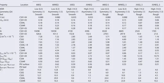
A total of eight experiments were performed (Table 1), varying three parameters: width-to-depth ratio (WDR), discharge ratio (Qr), and bed roughness. Experiments were conducted with two different WDRs namely 6.3 and 14.3, the latter representing conditions found in natural systems such as the Cumberland Marshes, Canada [Edmonds and Slingerland, 2008] and the Columbia River, Canada [Kleinhans et al., 2012]. For these ratios, water depths of 80 and 35 mm were used, abbreviated as 80xxx and 35xxx herein. Both equal (nnEQ) and unequal (nnNEQ) discharge divisions were examined; discharge ratios ofQr51 and aboutQr51.5 were used. Downstream weirs were used to control discharge ratio and water depth in each bifurcate. For the equal discharge division runs, discharge and weir heights were adjusted to acquire the required water depth and uniform flow conditions. Experiments with unequal discharge division were always run with the same discharge as their equal counterparts; in these runs uniform flow was acquired by varying weir heights. The backwater adaptation length [Ribberink and Van Der Sande, 1985;Parker, 2004 also seeKleinhans et al., 2013, for importance in bifurcations, sometimes named backwater length or backwater effect], estimated bykbw5h=3S(his water depth,Schannel slope), equals 27 m for the low width-to-depth ratio, and 12 m for the high width-to-depth ratio experiments. These values are longer than the entire flume, justifying using downstream weirs to control the division of water at the bifurca-tion. Individual runs were repeated to allow data collection with different techniques.
[image:5.630.51.584.120.390.2]All the experiments described above were conducted with a smooth bed as well as with a rough bed; experiments with a rough bed are indicated with the suffix _S for sediment. For the experiments with a
Table 1.Experiment Design Parameters and Flow Propertiesa
Property Location
Run
80EQ 80NEQ 35EQ 35NEQ 80EQ S 80NEQ_S 35EQ_S 35NEQ_S
WDR Low (6.3) Low (6.3) High (14.3) High (14.3) Low (6.3) Low (6.3) High (14.3) High (14.3) Symmetry (Qr) Symmetry (1) Asymmetry (1.5) Symmetry (1) Asymmetry (1.5) Symmetry (1) Asymmetry (1.5) Symmetry (1) Asymmetry (1.5)
Bed Smooth Smooth Smooth Smooth Rough Rough Rough Rough
H(m) CS01-04 0.080 0.080 0.035 0.035 0.080 0.080 0.035 0.035
Uxav(m/s) CS01-03 0.18 0.18 0.16 0.15 0.14 0.15 0.09 0.06
CS04L 0.18 0.14 0.16 0.10 0.14 0.12 0.07 0.04
CS04R 0.18 0.23 0.16 0.18 0.15 0.17 0.06 0.06
Fr CS01-03 0.20 0.20 0.28 0.26 0.16 0.17 0.15 0.10
Re CS01-03 10298 10358 4720 4396 8320 8605 2524 1765
We CS01-03 426.6 431.5 152.8 132.5 278.5 297.9 43.9 21.6
Q(m3/s
31023) CS01 7.28 7.22 2.85 2.69 5.71 6.02 1.65 1.16
CS02 7.14 7.16 2.83 2.62 5.74 6.00 1.41 1.10
CS03 7.03 7.21 2.81 2.60 5.90 5.91 1.49 0.92
CS04L1R 7.08 7.25 2.78 2.49 5.80 5.87 1.17 0.91
CS04L 3.56 2.71 1.37 0.88 2.85 2.40 0.61 0.36
CS04R 3.52 4.54 1.41 1.61 2.95 3.47 0.55 0.55
Qrms(m3/s31023) CS01-04 0.09 0.03 0.03 0.07 0.07 0.06 0.17 0.11
Qrmsð%Þ CS01-04 1.33 0.46 0.89 2.72 1.24 1.08 12.16 10.73
QrðQright=QleftÞ CS04 0.99 1.67 1.03 1.83 1.03 1.45 0.90 1.51
Qright=Qtotal CS04R 0.50 0.63 0.51 0.65 0.51 0.59 0.47 0.60
qsurf;right=qsurf;total PIV surface 0.51 0.62 0.50 0.56 0.49 0.55 0.50 0.51
qbed;right=qbed;total PIV bed 0.52 0.71 0.50 0.68
jC^j CS01 15.4 12.8 5.5 0.9 8.5 9.0 2.1 4.0
CS02 14.6 10.8 1.2 1.0 6.0 8.1 1.3 4.3
CS03 12.7 10.3 0.9 1.5 6.8 10.0 2.9 4.5
CS04L 18.0 29.9 9.9 7.1 24.4 31.5 8.4 8.5
CS04R 13.1 16.3 8.2 4.0 27.6 23.9 5.4 10.2
a
rough bed, a 15 mm thick immobile layer of 3–8 mm (D5055 mm) white gravel was installed at the bed of the model. The same water depths and discharge ratios were used for the runs with sediment; water levels were measured relative to the top of the gravel bed to retain the same width-to-depth ratio. To ensure uni-form flow, but to retain the same WDR, experiments 35EQ_S and 35NEQ_S and experiments 80EQ_S and 80NEQ_S were run at about 60% and 80% of the discharge of their smooth-bed counterparts, respectively. This reduced discharge is caused by slower flow induced by the increased roughness.
2.2. Data Acquisition
2.2.1. Flow Velocity Vectors (UDVP)
A series of measurements were taken from a total of four cross sections distributed throughout the model domain (Figure 1c). 1-D flow velocities were measured sequentially in the streamwiseUx, cross-streamUy
and verticalUzdirections at each cross section (Figure 1c) using an ultrasonic Doppler velocity profiling (UDVP) system [Takeda, 1991, 1995]. A Met-Flow UVP-XW ultrasonic velocity profiler was used to record a multiplexed signal from an array of 4 MHz ultrasonic transducers. The locations of the measurements were chosen such that the individual signals could be combined into time-averaged 3-D flow velocity vectors for each cross section. The positions of the transducers are described in detail in the following paragraphs (also see Figure 1d).
For the measurement of bothUxandUy, seven UDVP transducers were used. These transducers were placed at a distance of 10 mm from each other. For the lower WDR runs (runs 80xxx), all seven transducers were used to measure flow velocities. For the higher WDR runs (runs 35xxx), only three transducers were submerged due to the shallower water depth. For the measurement of cross-stream velocities, the trans-ducers were mounted on the outside of the Perspex flume wall and sounded the flow using acoustic cou-pling gel to prevent distortion of the acoustic signal through the flume walls. In the upstream section, the cross-stream measurements were repeated from both sides. Streamwise velocities were measured by insert-ing the stack of probes in the flow 100 mm downstream of the actual position of the cross section in order to minimize the influence of the probe on the measured flow field. Measurements forUxwere taken at 16 locations per cross section in the upstream channel (see Figure 1d) and at eight locations per cross section in the bifurcate channels (effectively splitting the measurement location shown in Figure 1d). For the mea-surement ofUz, 16 UDVP transducers were used in the upstream channel and 8 in the bifurcate channels. Transducers were mounted to be only slightly submerged. Locations corresponded with the location ofUx
measurements.
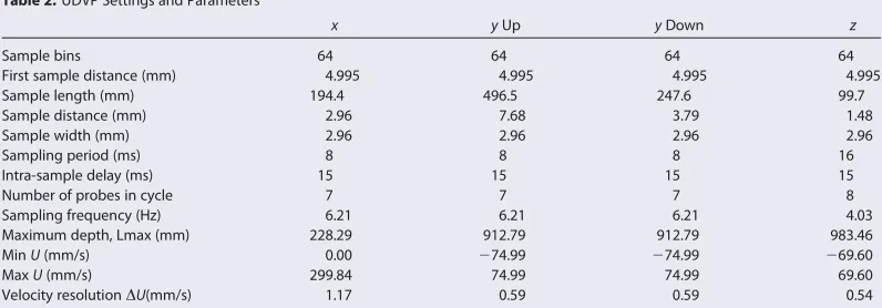
[image:6.630.184.582.108.247.2]The measured streamwise flow velocitiesUxwere in the range of 40–240 mm/s for the low-WDR runs and 10–200 mm/s for the high-WDR runs. The majority of cross-stream flow velocitiesUywere in the range of 210 to110 mm/s for the low-WDR runs and25 to15 mm/s for the high-WDR runs. Vertical flow veloc-itiesUzwere in the range of24 to14 mm/s for the low-WDR runs and21 to 1 mm/s for the high-WDR runs. These fell well within the measurable range (Table 2),UxandUywere high compared to the flow velocity resolution. Values forUzcome quite close to the minimum measurable value in the high-WDR runs.
Table 2.UDVP Settings and Parametersa
x yUp yDown z
Sample bins 64 64 64 64
First sample distance (mm) 4.995 4.995 4.995 4.995
Sample length (mm) 194.4 496.5 247.6 99.7
Sample distance (mm) 2.96 7.68 3.79 1.48
Sample width (mm) 2.96 2.96 2.96 2.96
Sampling period (ms) 8 8 8 16
Intra-sample delay (ms) 15 15 15 15
Number of probes in cycle 7 7 7 8
Sampling frequency (Hz) 6.21 6.21 6.21 4.03
Maximum depth, Lmax (mm) 228.29 912.79 912.79 983.46
MinU(mm/s) 0.00 274.99 274.99 269.60
MaxU(mm/s) 299.84 74.99 74.99 69.60
Velocity resolutionDU(mm/s) 1.17 0.59 0.59 0.54
a
For every measurement location, a total of 512 samples were collected. This value was determined using a method to estimate the optimal record length for turbulent flow [Buffin-Belanger and Roy, 2005]. This was achieved via analysis of convergence of the measured velocity to a mean value. Each transducer was set to record 1-D velocities in a profile at 64 distances from the probe. These profiles spanned different lengths for the different measurement orientations and locations: 596.5 mm for cross-stream measurements in the upstream channel, 247.6 mm for cross-stream measurements in the downstream channels, 194.4 mm for streamwise measurements and 99.7 mm for vertical measurements (see Table 2 for full set of properties). For the cross sections in the upstream channel, the cross-stream velocity was measured sequentially from both sides of the channel. At every vector location in each section, the two available values for the cross-stream component taken from either side were compared. If the difference of the two values was within one standard deviation of all cross-stream values, the mean of these values was used. Otherwise, the value with highest magnitude was used. This procedure was followed because in the cross-stream data, vertical bands with zero flow velocities were present in some of the data. It is likely that acoustic reflections from the opposite flume wall induced negative interference and caused these bands.
2.2.2. Near-Bed and Surface Flow Fields (Particle Image Velocimetry)
For all model runs, Particle Image Velocimetry (PIV) [seeAdrian, 1991, 2005] was used to record 2-D near-surface flow velocity vectors in the streamwiseUxand cross-streamUydirections. This was achieved through introduction of about 15,000 floating particlesðqs5660 kg=m3;d52:022:5 mm
Þ. Additionally, for runs with a smooth bed, near-bed velocities were also measured using PIV using about 10,000 denserðqs5 1360 kg=m3;d52:5 mmÞparticles. In contrast to classic PIV techniques with neutrally buoyant small
ticles and laser sheets, we applied PIV methods to slightly larger floating surface particles and sinking par-ticles at the channel bed [cf.Jodeau et al., 2008;Blanckaert et al., 2013]. Note that the PIV data were collected in separate, repeated runs and not simultaneously with the UDVP data.
For both the near-surface and near-bed measurements, PIV involved uniformly feeding black particles into the inlet channel over a period of about 10 s. A digital SLR camera with High Definition (HD) video capabil-ities (Canon EOS 550D) with a low-distortion wide angle lens (Canon EF-S 10–22 mm at 20 mm) was used to record the movement of the particles during the run. The camera was mounted perpendicular to the flume in the center of the channel just upstream of the bifurcation head (Figure 1c). The camera was set to shoot HD video (108031920 at 29.97 fps). Three 500 W halogen lamps, shielded to prevent reflections at the water surface, illuminated the measurement section. Single frames were extracted from 15 to 20 s of video from each run, resulting in 450–700 individual frames.
For all runs, images of different water levels were used to create image masks to remove areas outside the actual flow field. These masks represent the width of the flume for the different water levels, and effectively correct for vertical relief-displacement. Since the water surface had a low gradient, the camera was horizon-tal and centered above the flume, and its lens introduced minimal distortion, correction of barrel or per-spective distortion was not necessary. Perper-spective distortion was most significant at the edges of frames, where the angle of incidence was most oblique, but it was minimal directly beneath the camera, which cov-ered the region surrounding the bifurcation. A rectangular region centcov-ered on the inlet channel with the bifurcation head as a fixed point was cropped out of the masked image. The resulting image was converted to 8-bit gray scale, inverted and a pixel value threshold was then applied to remove irregularities introduced by the bed and walls. Lighting irregularities were minimal relative to the high contrast between the black particles and white background.
from the local mean being removed from the data set. This filtering resulted in the removal of about 10% of the vectors in the surface measurements for the smooth-bed runs and about 35% of the rough-bed runs. For the near-bed measurements of the smooth-bed runs, about 5% of the vectors were filtered. The quality of this method seems to be related to artifacts introduced by visible shadows caused by the gravel in the setup. The mean values per time series were used in further analysis. Note that no spatial filtering or any form of interpolation was performed on the data.
2.3. Data Analysis
2.3.1. Discharge and (Depth-) Averaged Velocities
The measured UDVP data were used to calculate cross-sectional discharge and average flow velocity vec-tors. The average flow velocity was calculated for each measured cross-sectioncsand at each measured depth profiley. The cross-sectional dischargeQcs(m3/s) was calculated by summing the products of stream-wise flow velocity measurementsUx(m/s) and their effective areaa(m2):
Qcs5 X
ny
y51
Xnz
z51
Uxy;zay;z
(1)
wherenyandnzare the number of depth profiles and vertical locations in each profile, respectively.ais cal-culated from the distances from the centers between measurement locations or the flow boundaries at the outer edges. The cross-sectional averaged velocityUav;csðm=sÞis the discharge through that cross section (Qcs) divided by cross-sectional areaA5WHðm2Þ:
Uav;cs5Qcs=A (2)
The discharge passing through the upstream sections CS01, CS02, and CS03, and the summed discharge of both downstream sections CS04L and CS04R were evaluated for continuity by calculating the root-mean-square (RMS) deviation from the mean dischargeQof all four sections:
Qrms5
ffiffiffiffiffiffiffiffiffiffiffiffiffiffiffiffiffiffiffiffiffiffiffiffiffiffiffiffiffiffiffi 1
n
Xn
cs51
Q2Qcs
ð Þ2
s
(3)
wherenis the number of measured cross sections. At each measured vertical profiley, the discharge per unit widthqxy(m/s) was calculated in a similar way as the cross-sectional discharge:
qxy5 Xnz
z51
Uxy;zhz
(4)
wherehzis the effective height of each measurement. For the depth-averaged flow velocity vectorsUxav;y, the discharge per unit widthqxywas divided by the flow depthH:
Uxav;y5qxy=H (5)
Equations (4) and (5) were also applied to attain depth-averaged cross-stream flow velocitiesUyav;yby sub-stituting streamwise flow velocitiesUxby cross-stream flow velocitiesUy.
2.3.2. Streamwise Circulation and Planar Vorticity
UDVP measurements were used to calculate the streamwise circulation at each cross section. PIV data were used to calculate the planar vorticity field for both the surface and the near-bed measurements.
C5 ð
z ð
y
xdydz (6)
whereC(m2/s) is the circulation andx(rad/s) is the vorticity, which is defined as the curl of the vector velocity field:
x5r3~u (7)
where~uis the 2-D vector field of cross-stream and vertical flow velocitiesUyandUzfrom UDVP measurements.
In order to compare the circulation for different cross sections, the circulation is computed using the abso-lute values of the vorticity (x5jxjin equation (6)). The vorticity is normalized using the method ofvan Balen[2010, p. 77]:
jC^j5jxjH=ðAUav;csÞ (8)
wherejC^jis the absolute normalized circulation.
Details of the secondary flow structure are also shown by the planar vorticity (in thex-yplane) using equa-tion (7), but using cross-stream flow velocities (Uy) and downstream flow velocities (Ux) for vector field~u, taken from PIV measurements of the surface flow and near-bed flow.
2.4. Data Quality
2.4.1. Development of Turbulence
We analyzed the UDVP data at CS01 to ascertain whether the flow was fully turbulent. Turbulent flow condi-tions result in a logarithmic velocity profile. We tested if such profile existed in the measured flow velocities. At each vertical profiley, we applied a logarithmic regression to predict the streamwise flow velocityUx^ as a function of the height above the bedz:
^
UxðlogðzÞÞ5a01a1logðzÞ (9) wherea0anda1are linear regression coefficients. We analyzed these profiles visually and we indicate how good the data fits the model with the coefficient of determinationR2, which is calculated as:
R2512 X
UxðzÞ2Ux^ ðzÞ
2
X
UxðzÞ2Ux
2 (10)
whereUxis the average flow velocity in the profile under consideration.
2.4.2. Scaling Assessment
We used the Froude number, Reynolds number, and Weber number to evaluate the hydraulic behavior of our experiments. We evaluated these values from UDVP measurements in the upstream section of the experiment. The Froude number (Fr) determines whether the flow is affected by downstream or upstream disturbances, respectively, subcriticalðFr<1Þor supercriticalðFr>1Þflow. Subcritical flow conditions are desirable.
Fr5 Uffiffiffiffiffiffi
gH
p (11)
Re5UR
m (12)
whereRis the hydraulic radius (m),R5ðHWÞ=ð2H1WÞ;mis the kinematic viscosity of water (m2/s),
m431025=ð201tÞ, wheretis the temperature (18C for the current experiments). We aimed for turbulent flow in our experiments.
Weber (number We) shows the relation between inertia and surface tension forces [Peakall and Warburton, 1996]. Critical values for the Weber number are uncertain and vary from 10 to 100, so we aim for values above this range.
We5U
2qH
r (13)
whereqis the density of water andris the surface tension. We used an estimate ofr5631023N=m in our
experiments as opposed to the value of 731022N=m for water because we added soap in the water to
reduce the surface tension.
3. Results
3.1. General Flow Structure
The following key flow field properties were derived from UDVP data (Table 1): (1) all equal weir runs had equal (50/50) discharge division; (2) all unequal weir runs had a discharge division close to 40/60. The meas-ured discharge was less uniform for the shallower runs with a rough bed (Table 1,QRMS), which is probably due to the higher levels of noise present in the UDVP measurements for these runs.
3.2. Effect of Flow Division on Flow Structure
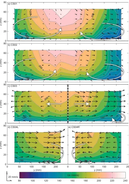
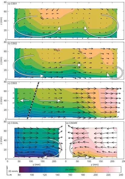
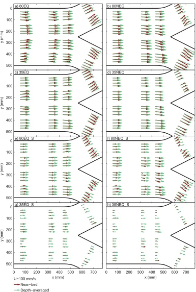
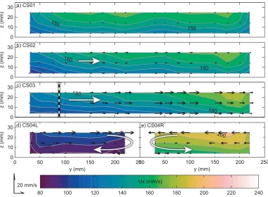
In the low-WDR smooth-bed runs with equal discharge division (Run 80EQ), the high velocity core was positioned in the center of the channel (Figure 2). In the unequal discharge division case (80NEQ), the flow velocity core was located to the right-hand side in the two downstream cross sections (Figure 3), the side with the gradient advant-age and largest discharge. In both the equal and unequal cases (80EQ, 80NEQ), two opposed secondary flow cells were present in the channel upstream of the bifurcation. These cells flowed toward the center of the channel at bed level and toward the banks at the water surface (Figures 2a, 2b and 3a, 3b). However, in the unequal discharge division case, the cell at the side of the channel with the highest discharge was smaller (Figures 3a and 3b). In both cases, the division of flow becomes visible in CS02 and dominates the flow structure in CS3. In the latter, the rota-tional flow cells are almost absent (Figures 2c and 3c). For a large portion of the width (about 80%) in the unequal discharge division case, the flow structure caused the near-bed velocities to be oriented toward the channel with the water surface gradient advantage (Figures 3c and 4b). Note that a flow direction toward the right channel does not mean that this flow indeed enters the right channel, as we will discuss later.
In both bifurcate channels, most velocity vectors were consistently directed toward the inner bank while the near-bed vectors were directed toward the outer banks (Figures 2d, 2e and 3d, 3e). This flow structure had an inverse direction of rotation compared to the flow cells upstream of the bifurcation.
The PIV vectors obtained for the near-surface and near-bed flow reveal a more detailed flow field in the hor-izontal plane than the UDVP data (Figures 5 and 6), especially in the area just upstream of the bifurcation (the downstream-most UDVP section (CS03) is located atx5431 mm in Figures 5 and 6). In this zone, the flow divergence and steering into the bifurcate channels becomes even stronger than at the locations observed with UDVP data (Figure 5). Moreover, near-bed flow accelerates closer to the bifurcation (Figures 6b and 6d). Indeed, just upstream of the bifurcation (x5550 mm, Figure 6) the near-bed velocity vectors were almost perpendicular to the outer banks in both cases with unequal discharge division (nnNEQ).
0
100
200
300
400
500 a) 80EQ
y (mm)
b) 80NEQ
0
100
200
300
400
500 c) 35EQ
y (mm)
d) 35NEQ
0
100
200
300
400
500
e) 80EQ_S
y (mm)
f) 80NEQ_S
0 100 200 300 400 500 600 700
0
100
200
300
400
500
g) 35EQ_S
x (mm)
y (mm)
0 100 200 300 400 500 600 700
h) 35NEQ_S
x (mm) U=100 mm/s
[image:13.630.192.577.93.665.2]Near−bed Depth−averaged
(Table 1); and (3) the majority of this division of near-bed flow occurred within a distance of about one chan-nel width upstream of the bifurcation (Figure 7b).
3.3. Effect of Width-to-Depth Ratio on Flow Structure
Similar flow features described above were also observed in the higher WDR runs 35EQ and 35NEQ (see Fig-ures 8, 9 and 4c, 4d), although some differences exist. There is no high flow velocity core in the middle of the channel, but the highest flow velocities are spread over a larger part of the channel (Figure 8c). More-over, there are two locations with higher velocities, one in the left and one in right part of the upstream channel, which align with the highest velocity cores in the bifurcate channels (Figures 8d and 8e). Also, in the unequal discharge case, the streamwise velocities develop toward one core of flow velocity on the side of the channel with the largest discharge (Figure 9c). The secondary flow structures upstream of the bifurca-tion consist of two counter-rotating flow cells in the middle of the channel flowing toward the banks near the bed (Figure 8a). Additionally, a third and fourth flow cell was present near the banks, with flow directed toward the banks near the water surface (Figure 8a).
[image:15.630.171.581.96.443.2]The secondary flow structure at the center of the channel in the high-WDR runs mirrored that observed in the low-WDR runs. In addition, downstream of the bifurcation, the secondary cells did not change their sense of rotation and instead continued to rotate in the same orientation as upstream of the bifurcation, with upwelling at the location of the highest streamwise velocity. These flow cells were not observed upstream of the bifurcation in the unequal discharge division high-WDR run 35NEQ (Figure 9). We speculate that the divergence close to the bifurcation and the flow cells within the bifurcate channels are comparable to the structure observed in the low-WDR runs and suppress the flow cells closer toward the bifurcation (Figures 8b and 8c). Note that the orientation of the secondary flow structures was largely inferred from the
cross-stream velocities because the vertical velocities were close to or less than the measurement resolution.
There was no clear difference in the direction of near-bed and depth-averaged flow (Figure 4). However, a divergence between near-bed and surface water was observed in the zone just upstream of the bifurcation (betweenx5400 mm and the bifurcation) in both the low-WDR runs (80EQ, 80NEQ, Figures 5a and 5b) and high-WDR runs (35EQ, 35NEQ, Figures 5c and 5d). This diversion extended farther upstream and was signifi-cantly more pronounced in the low-WDR runs. The near-surface velocities are affected by the unequal dis-charge distribution at a distance of about one channel width upstream of the bifurcation in the low-WDR run (80NEQ, Figure 7b) and about half a channel width in the high-WDR run (35NEQ, Figure 7b). Interest-ingly, the low-WDR has less impact upon near-bed cross-stream flow velocities than on the near-surface flow. This effect is shown in terms of flow division (Figure 7 and Table 1): in the high WDR run (35NEQ), a larger proportion of the near-surface flow enters the bifurcate channel with a gradient advantageðqsurf;right=
qsurf;total562%Þwhereas in the low-WDR run this is somewhat lowerðqsurf;right=qsurf;total556%Þ. The same holds for near-bed flow, but with a smaller difference observed between the two runs
(qbed;right=qbed;total571% andqbed;right=qbed;total568% for runs 80NEQ and 35NEQ, respectively).
3.4. Flow Circulation
Upstream of the bifurcation, there were two counter-rotating flow cells with upwelling flow in the middle of the channel in the low-WDR runs. These cells were symmetrical in the symmetrical bifurcation (Figure 2a) and were unequal in size in the asymmetrical bifurcation (Figure 3b). In the high-WDR runs, two counter-rotating flow cells with downward flow in the middle and two weaker flow cells with downward flow near
1.0
0.9
0.8
0.7
0.6
0.5
0.4
0.3
0.2
0.1
0.0
0.0
0.1
0.2
0.3
0.4
0.5
y/W
x/W
b) unequal discharge division (xx=NEQ)
80xx
35xx
80xx_S
35xx_S
80xx_bed
35xx_bed
0.4
0.5
0.6
a) equal discharge division (xx=EQ)
[image:16.630.183.582.91.437.2]x/W
Figure 9.3-D velocity components (UDVP data) for run 35NEQ, see Figure 2 for caption.
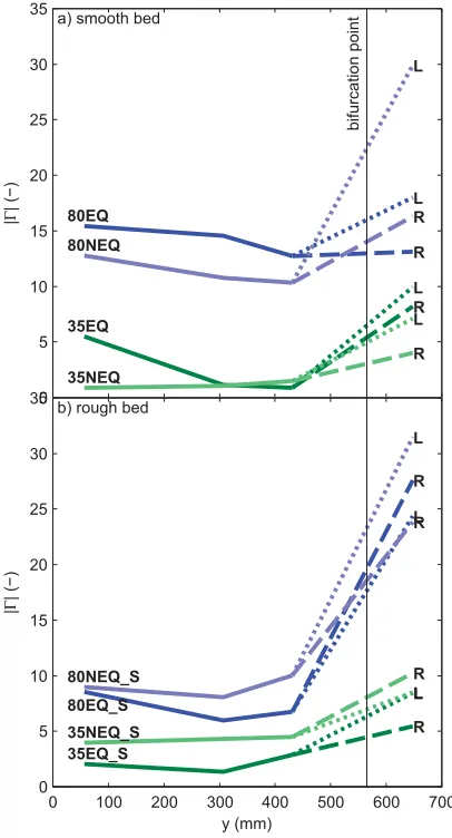
the banks on either side were observed in the symmetrical run (Figure 8a), but this structure was not observed in the unequal discharge run (Figure 9a). In all cases, these flow cells were suppressed by strong divergence closer to the bifur-cation. Downstream of the bifurcation, a single flow cell was present in each bifurcate channel with flow toward the outer bank near the channel bed (Fig-ures 2d, 2e, 3d, 3e, 8d, 8e, and 9d, 9e). The magnitude of circulation consis-tently increased downstream of the bifurcation in all runs (Figure 10). Earlier results [Thomas et al., 2011] already show the inversion of direction and increase in magnitude of flow rotation in the bifurcate channel. This effect is attributed to super-elevation of the water surface at the bifurcation point.
The low-WDR runs (80xx) had a higher relative circulation than the high WDR runs (35xx) (Figure 10). For unequal dis-charge division cases, the subordinate left channel (gradient disadvantage and thus lower discharge) had a 20–50% larger intensity of normalized circulation than the dominant right channel (Figure 10). In the equal discharge division cases, there were differences in circulation between the bifurcate channel, but these were small and not always stronger in the same channel (Figure 10). Perhaps the most notable difference was for 80NEQ, which is likely to had the strong-est transverse flow velocities because of the low-WDR and smooth bed.
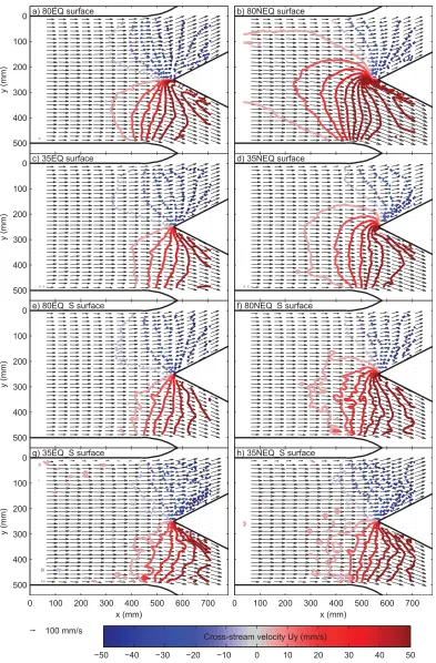
The planar vorticity of the near-surface flow field shows the presence of rotating cells in the smooth-bed runs (Figures 11a–11d). The general pat-tern corresponds with the flow structures observed in the UDVP data, with the presence of two counter-rotating flow cells in the low-WDR runs (Figures 11a and 11b) and the presence of two additional cells in the high-WDR runs (Figures 11c and 11d). The main vorticity pattern in the low-WDR runs corresponds with a high flow velocity core in the middle of the channel and slow flow on the sides, which results in rightward vorticity on the right-hand side of the channel and toward the left on the left-hand side. In the high-WDR runs, there is no concentrated velocity core in the middle of the channel, the high velocity is more spread over a larger area. In this case, the patterns of planar vorticity indicate multiple counter-rotating flow cells. In both cases, the planar vorticity pattern follows the streamline curvature. The pattern of planar vorticity in the near-bed flow (Figure 12) also shows a banded pattern. However, there are more small-scale features. These patterns do not resemble those observed in the surface data. Additionally, these patterns also show dividing and splitting circulation bands.
Spatially averaged vorticity (Figure 13) shows the cross-sectional average planar vorticity pattern in the upstream reach. The large-scale pattern for the low-WDR runs is consistent for both the equal and unequal discharge division and both smooth and rough bed runs (Figure 13a). This pattern is the result of the
[image:18.630.195.398.100.476.2]high-0 5 10 15 20 25 30 35 80EQ L R 35EQ L R 80NEQ L R 35NEQ L R bifurcation point | Γ | (−)
a) smooth bed
0 100 200 300 400 500 600 700
0 5 10 15 20 25 30 35 80EQ_S L R 35EQ_S L R 80NEQ_S L R 35NEQ_S L R | Γ | (−) y (mm) b) rough bed
flow velocity core in the center of the upstream channel which curves toward the outer banks and is con-sistent with the flow structures observed in the cross section. The vorticity pattern in the high-WDR runs shows local vorticity patterns superimposed on a large-scale vorticity pattern (Figure 13b). This pattern is
consistent with local flow structures, as also observed in cross-section data (Figures 8 and 9). Vorticity of the near-bed flow shows a local pattern without a large-scale structure (Figures 13c and 13d).
3.5. Effect of Bed Roughness on Flow Structure
In the runs with a rough bed (nnxxx_S), the deviations of the near-bed velocity from the depth-averaged velocity in the low-WDR rough bed experiments were similar to their smooth-bed counterparts (Figures 4e and 4f, 80EQ_S, 80NEQ_S). Flow velocities were lower in the rough bed cases. Additionally, the decrease in flow velocity toward the bed is stronger for the rough bed cases. The general flow structures were similar to those in their smooth-bed counterparts but were smaller in magnitude (Figures 5e–5h).
The high WDR, rough bed experiments (Figures 4g and 4h, 35EQ_S, 35NEQ_S) showed significant levels of noise induced by acoustic interference between the rough bed and the UDVP. Unfortunately, the near-bed flow field could not be quantified using PIV because of entrapment of particles in the bed sediment. In the rough bed runs, the upstream influence of the bifurcation extends for only half the distance observed in their smooth-bed counterparts. Near-surface flow is divided more equally between the distributaries (Figure 7 and Table 1,qbed;right=qbed;total555% for run 80NEQ_S) and almost equal in the higher WDR run
[image:20.630.180.590.96.443.2](qbed;right=qbed;total551% for run 35NEQ_S). Compared to the smooth-bed runs, similar vorticity patterns are visible in the rough bed cases, although these are noisier (Figures 11e–11h). The effect of bed roughness is dependent upon the WDR: in the low-WDR runs, both the smooth and rough beds show similar banding of comparable magnitude (Figure 13a) whereas in the high-WDR runs the rough bed shows similar banding, but at about a 2–4 times higher magnitude (Figure 13b, pale colored lines). This comparison shows that stronger flow structures emerged preferentially in channels with a larger width-to-depth ratio, but were reduced in channels with a larger ratio of roughness length to water depth.
4. Discussion
4.1. Scaling Assessment and Robustness of Methods
In all experimental runs, the flow was subcritical with Froude numbers between 0.1 and 0.3 (Table 1). The Reynolds number was well above the threshold for turbulent flow (Re>2000) in all low-WDR runs and in the smooth-bed high-WDR runs.Revalues for the high-WDR runs with rough bed, equal discharge division (35EQ_S) are closer to, but still above 2000. Run 35NEQ_S had a Reynolds number slightly below 2000 (Table 1). The same is shown by the flow velocity profiles at the most upstream cross section: the measured flow velocity profiles show a well-developed logarithmic profile in all low-WDR runs (Figure 14a) and in the high-WDR, smooth-bed runs (Figure 14b, closed symbols). The high-WDR, rough bed runs show more scat-tered velocity profiles (Figures 14b and 14c, open squares), which is most probably due to noise in the measurements due to the high amount of acoustic scattering on the rough bed and the limited water depth. Nevertheless, the Reynolds number is in the upper end of the transitional regime and the velocity profiles show no indication of laminar flow so we believe these experiments to have had fully turbulent flow.
Deviations from the logarithmic profile are apparent close to the flume wall (Figure 14a, probe 1). The devia-tion from a logarithmic profile is visible in all measurements and most prominent in the smooth bed, low-WDR runs (Figure 14c, closed circles). This wall friction effect is expected and is perhaps even more impor-tant in natural channels.
In small-scale experiments, surface tension might have an effect on the dominant processes. In our experi-ments, however, the relative importance of the fluid’s inertia to the surface tension is very low as the Weber number is above the critical value of 100 for most runs and well above 10 for the high-WDR, rough bed cases. Note that the reported critical values are not consistent [Peakall and Warburton, 1996].
We compared the streamwise velocity from UDVP measurements closest to the water surface to the surface PIV data at the same location (Figure 14d). Note that these two methods do not measure exactly the same flow in terms of time and space. However, the comparison is useful in that it provides a way to see whether
−1 −0.5 0 0.5 1
vorticity (rad/s)
a) low−WDR surface
80EQ 80NEQ 80EQ_S 80NEQ_S
b) high−WDR surface
35EQ 35NEQ 35EQ_S 35NEQ_S
0 0.2 0.4 0.6 0.8 1
−1 −0.5 0 0.5 1
x/W
vorticity (rad/s)
c) low−WDR near−bed
80EQ_bed 80NEQ_bed
0 0.2 0.4 0.6 0.8 1
x/W d) high−WDR near−bed
[image:21.630.204.563.97.366.2]35EQ_bed 35NEQ_bed
there are issues with any of the data. Most measurements are close to being equal, with the majority of PIV data giving slightly higher values, except in the case of the rough bed high-WDR runs where the UDVP data is noisy.
4.2. Implication for Bifurcation Instability
[image:22.630.261.502.101.597.2]Flow structure at bifurcations is determined by (1) flow forcing by streamline curvature, angular divergence upstream, and through a bifurcation and related zones of flow separation [e.g.,Ramamurthy et al., 2007]; (2)
Figure 14.(a and b) Measured streamwise velocity profiles (symbols) and logarithmic fit (lines) at CS01 at probe location 1 (next to wall), 4 and 8 (near-center) for all (a) low-WDR runs and (b) high-WDR runs. The data for Probes 4 and 8 are horizontally offset for visual clarity. Open symbols show the experiments with rough bed, pale colors are the unequal discharge division runs. (c) The coefficient of determina-tion (R2) of the logarithmic fit of flow velocities for all probes in CS01, shown against normalized distance to the wall, where the flume wall
the width-to-depth ratio and flow field inertial and momentum forces [e.g.,Bradbrook et al., 2001;Parsons et al., 2007]; (3) flow field super-elevation and related pressure gradient terms [e.g.,Shettar and Keshava Murthy, 1996]; (4) backwater surface slopes; and (5) topographic forcing by the bed [e.g.,McArdell and Faeh, 2001;Bolla Pittaluga et al., 2003;Kleinhans et al., 2008]. In this paper, two-independent flow measurement techniques have been used to quantify flow fields in a morphologically symmetrical experimental bifurca-tion. Flow structures develop that can significantly modify the near-bed flow direction at a distance of up to one channel width upstream of the bifurcation head. The character of the flow was turbulent and highly subcritical with strong backwater effects. Data obtained from control experiments with equal discharge par-titioning do not show asymmetric near-bed flow but do have some flow structures that contain counter-rotating transverse-vertical cells upstream of the bifurcation in addition to a clear signal of the bifurcating flow closer to the bifurcation. In the experiments with unequal discharge partitioning, the near-bed trans-verse flow was directed toward the bifurcate channel which had a gradient advantage and largest dis-charge. About 80% of the near-bed flow entered the larger channel. Furthermore, as expected, the
transverse flow component is larger for channels with larger water depth relative to channel width and rela-tive to the characteristic length of bed roughness. This flow structure upstream of the bifurcation is caused by flow curvature toward the bifurcate channels at the bifurcation. Such upstream influence is also observed in curved channels and may be the result of the actual flow curvature itself [Jamieson et al., 2010], or the result of backwater effects [Blanckaert et al., 2013]. Downstream of the bifurcation, the flow structure shows a pattern that is consistent with plunging water resulting from super-elevation at the bifurcation point, as shown byThomas et al. [2011].
In classical analyses of the stability of a perfectly symmetrical bifurcation, a perturbation to the bed level or water depth is introduced either in one of the distributaries or just upstream of the bifurcation [Wang et al., 1995;Bolla Pittaluga et al., 2003;Kleinhans et al., 2008]. Such a perturbation may grow or dampen depend-ing on the channel width-to-depth ratio and sediment mobility. A growdepend-ing perturbation may eventually lead to the closure of one of the bifurcate channels, i.e., the bifurcation is unstable. In the present paper, we document laboratory flume experiments in which we perturbed the bifurcation by changing the energy gradient in the bifurcate channels. Theoretically, this should always lead to the enlargement of the channel receiving the most discharge when the bifurcation is otherwise symmetrical. Our experimental findings sug-gest that the destabilization of a morphologically perfectly symmetrical bifurcation has a pronounced influ-ence on the near-bed flow over a distance of about one channel width upstream of the bifurcation, which may influence the bifurcation stability. This length scale is in agreement with the length scales and model concepts ofBolla Pittaluga et al. [2003] andKleinhans et al. [2008]. However, in these models, the upstream length of bifurcation influence is assumed to be the result of an upstream extension of topographic forcing by the bed [e.g.,McArdell and Faeh, 2001;Bolla Pittaluga et al., 2003;Kleinhans et al., 2008], which was absent in our experiments. In our case, the dividing line between near-bed flow that enters the dominant channel and near-bed flow that enters the subordinate channel is strongly curved (Figure 7). Thus, the frac-tion of upstream channel width that contributes water to the dominant bifurcate channel is much larger than expected on the basis of the relative discharges of the bifurcate channels. This novel result is not included within the depth-averaged model concepts used in bothBolla Pittaluga et al. [2003] andKleinhans et al. [2008]. The implication is that linear stability analyses of perturbed bifurcations based on depth-averaging require modification for the flow structure induced by discharge asymmetry, which is the result of a perturbation in one of the downstream channels.
The observed near-bed flow structure upstream of perturbed bifurcations has an unexpected ramification for the breakdown of symmetry of river bifurcations. In our experiments, near-bed flow is directed toward the dominant bifurcate. Such flow structure may cause an increase of sediment supply into this dominant channel. For example, for experiments where the dominant bifurcate received about 60% of the total dis-charge, about 70% of the near-bed flow was going into this bifurcate (Figure 7). We expect a similar effect on bed load partitioning in bifurcations.
upstream of the bifurcation will initially lead to sedimentation in the dominant channel because of flow convergence, but also sedimentation upstream of the subordinate channel distributary because of flow divergence. As a result, the dominant channel may aggrade initially, even if it eventually enlarges [e.g., Ber-toldi and Tubino, 2007;Bolla Pittaluga et al., 2003;Edmonds and Slingerland, 2008;Federici and Paola, 2003;
Kleinhans et al., 2008;Miori et al., 2006]. The flow structure observed in our experiments may thus cause sta-bilization of a symmetrical but perturbed bifurcation. This negative feedback has not been described before.
The question is: how important is this negative feedback in natural bifurcations? It could be argued that the sediment transport capacity of the dominant bifurcate channel would increase nonlinearly with discharge. However, the analyses ofWang et al. [1995] andBolla Pittaluga et al. [2003] demonstrate that the ratio of sediment transport in the two bifurcatesQs;right=Qs;left5 Qright=Qleft
k
, wherekis unity in the absence of a transverse bed slope and planimetric perturbation. In principle,kis to be determined empirically, but three-dimensional flow and sediment transport modeling has demonstrated thatkis approximately unity for much of the lifetimes of bifurcations formed in mobile beds [Kleinhans et al., 2008]. Herek51 means that sediment is partitioned over the downstream channels proportionally to their widths. This work was based on modeling idealized but asymmetrical bifurcations with an initially flat bed [Kleinhans et al., 2008]. There were indeed fluctuations in discharge partitioning after the start of all model runs, particularly in runs where the bifurcate channels were nearly balanced by, on the one hand, a gradient advantage for one channel, but on the other hand an advantage for the other channel caused by an upstream bend with helical flow upstream of the bifurcation that favored the subordinate channel. The models show that initially sediment always deposited in one of the channels such thatkis offset as the dominant bifurcate channel initially receives relatively more sediment despite the presence of a bend [Kleinhans et al., 2008, Figure 9]. This can be expressed empirically as:
Qs;right=Qs;left5a Qright=Qleft
k
(14)
wherea<1. In the numerical model, the ultimate bifurcation condition was asymmetrical in the manner expected from gradient or upstream bend advantage, but the evolution toward this state was delayed by the negative feedback of flow structure.
In short, previous numerical modeling work supports our hypothesis that bifurcations with subcritical flow, perturbed by asymmetrical downstream discharge conveyance, have a flow structure that may result in ele-vated sediment transport into the dominant channel, providing a negative feedback on the onset of bifur-cation destabilization. Given that the transverse bed slope upstream of the bifurbifur-cation only overcomes the initial flow and sediment attraction of the advantaged channel in a later stage, we hypothesize that balanc-ing potentially occurs when the transverse bed slope development is limited whilst the imbalance between channel width and flow discharge is large. In other words, balancing flow attraction and sediment attraction is most likely to occur where there is a large gradient or bend advantage for one channel, leading to higher discharge, whilst the other channel is equally wide or wider but has a lower discharge. Other important fac-tors are the roughness of the channel and the width-to-depth ratio of the channel, as these suppress the transverse flow and therefore the sediment attraction of the dominant channel.
The hitherto unidentified effect could lead to unexpected sedimentation in engineered bifurcations, for example, in small streams with newly created side channels. Such altered sedimentation patterns are likely in cases of low roughness. Furthermore, the flow structure and the inherited mixing of flow propagating into the downstream branches may be relevant for the aquatic chemistry of small bifurcating streams as commonly found in lowland areas, because it modifies the supply of dissolved oxygen, nutrients and organic matter. In addition, the reported effects of bifurcation perturbation on near-bed flow affect the bio-logically important benthic boundary layer.
5. Conclusions
width-to-depth ratios and either symmetrical or asymmetrical flow division forced by downstream water surface gradient.
Upstream of the bifurcation, counter-rotating flow structures emerged. In high width-to-depth ratio chan-nels, the number of flow cells increased. These flow cells were equal in size for bifurcations with equal dis-charge division, but asymmetrical for the bifurcation with unequal disdis-charge division. The flow cells diminished in strength with higher width-to-depth ratio and bed roughness. Closer to the bifurcation, flow divergence suppressed the flow structures.
Our experiments demonstrate that, under unequal discharge division, the flow is strongly curved toward the channel with the highest discharge over a length of about one channel width. The near-bed flow curva-ture was considerably larger than the surface flow curvacurva-ture, with the strongest curvacurva-ture just upstream of the bifurcation. These effects diminish with increasing width-to-depth ratio and increasing bed roughness.
Our results imply that a disproportionately large amount of sediment can be transported into the down-stream channel with the largest discharge. This could provide a negative feedback on bifurcation destabili-zation because the enhanced sediment input would reduce the expected erosion rate in that channel. This modifies the usual hypothesis that sediment division in a symmetrical bifurcation is proportional to channel width. This mechanism would act as a stabilizing effect on perturbed river bifurcations, which has not been taken into account in current theory.
References
Adrian, R. J. (1991), Particle-imaging techniques for experimental fluid mechanics,Annu. Rev. Fluid Mech.,23(1), 261–304, doi:10.1146/ annurev.fl.23.010191.001401.
Adrian, R. J. (2005), Twenty years of particle image velocimetry,Exp. Fluids,39(2), 159–169, doi:10.1007/s00348-005-0991-7. Bertoldi, W., and M. Tubino (2005), Bed and bank evolution of bifurcating channels,Water Resour. Res.,41, W07001, doi:10.1029/
2004WR003333.
Bertoldi, W., and M. Tubino (2007), River bifurcations: Experimental observations on equilibrium configurations,Water Resour. Res.,43, W10437, doi:10.1029/2007WR005907.
Blanckaert, K., M. G. Kleinhans, S. J. McLelland, W. S. J. Uijttewaal, B. J. Murphy, A. van de Kruijs, D. R. Parsons, and Q. Chen (2013), Flow sep-aration at the inner (convex) and outer (concave) banks of constant-width and widening open-channel bends,Earth Surf. Processes Landforms,38(7), 696–716, doi:10.1002/esp.3324.
Bolla Pittaluga, M., R. Repetto, and M. Tubino (2003), Channel bifurcation in braided rivers: Equilibrium configurations and stability,Water Resour. Res.,39(3), 1046, doi:10.1029/2001WR001112.
Bradbrook, K. F., S. N. Lane, K. S. Richards, P. M. Biron, and A. G. Roy (2001), Role of bed discordance at asymmetrical river confluences,J. Hydraul. Eng.,127(5), 351–368, doi:10.1061/(ASCE)0733-9429(2001)127:5(351).
Buffin-Belanger, T., and A. G. Roy (2005), 1 min in the life of a river: Selecting the optimal record length for the measurement of turbulence in fluvial boundary layers,Geomorphology,68(1–2), 77–94, doi:10.1016/j.geomorph.2004.09.032.
Edmonds, D. A., and R. L. Slingerland (2008), Stability of delta distributary networks and their bifurcations,Water Resour. Res.,44, W09426, doi:10.1029/2008WR006992.
Edmonds, D. A., and R. L. Slingerland (2009), Significant effect of sediment cohesion on delta morphology,Nat. Geosci.,3(2), 105–109, doi: 10.1038/ngeo730.
Federici, B., and C. Paola (2003), Dynamics of channel bifurcations in noncohesive sediments,Water Resour. Res.,39(6), 1162, doi:10.1029/ 2002WR001434.
Gui, L., and W. Merzkirch (1996), A method of tracking ensembles of particle images,Exp. Fluids,21(6), 465–468, doi:10.1007/BF00189049. Jamieson, E., G. Post, and C. Rennie (2010), Spatial variability of three-dimensional Reynolds stresses in a developing channel bend,Earth
Surf. Processes Landforms,35(9), 1029–1043, doi:10.1002/esp.1930.
Jodeau, M., A. Hauet, A. Paquier, J. Le Coz, and G. Dramais (2008), Application and evaluation of LS-PIV technique for the monitoring of river surface velocities in high flow conditions,Flow Meas. Instrum.,19(2), 117–127, doi:10.1016/j.flowmeasinst.2007.11.004.
Klaassen, G. J., and G. Masselink (1992), Planform changes of a braided river with fine sand as bed and bank material, in: Larsen, P. and N.E. Eisenhauer (Eds.), Sediment Management:Proceeding of 5th International Symposium on River Sedimentation, pp. 459–471, Karlsruhe, Germany.
Kleinhans, M. G., H. R. A. Jagers, E. Mosselman, and C. J. Sloff (2008), Bifurcation dynamics and avulsion duration in meandering rivers by one-dimensional and three-dimensional models,Water Resour. Res.,44, W08454, doi:10.1029/2007WR005912.
Kleinhans, M. G., K. M. Cohen, J. Hoekstra, and J. M. IJmker (2011), Evolution of a bifurcation in a meandering river with adjustable channel widths, Rhine delta apex, The Netherlands,Earth Surf. Processes Landforms,36(15), 2011–2027, doi:10.1002/esp.2222.
Kleinhans, M. G., T. Haas, E. Lavooi, and B. Makaske (2012), Evaluating competing hypotheses for the origin and dynamics of river anasto-mosis,Earth Surf. Processes Landforms,37(12), 1337–1351, doi:10.1002/esp.3282.
Kleinhans, M. G., R. I. Ferguson, S. N. Lane, and R. J. Hardy (2013), Splitting rivers at their seams: Bifurcations and avulsion,Earth Surf. Proc-esses Landforms,38(1), 47–61, doi:10.1002/esp.3268.
McArdell, B., and R. Faeh (2001), A computational investigation of river braiding, inGravel-Bed Rivers V, edited by M. Mosley, pp. 73–94, N. Z. Hydrol. Soc., Wellington.
Merzkirch, W., and L. Gui (2000), A comparative study of the MQD method and several correlation-based PIV evaluation algorithms,Exp. Fluids,28(1), 36–44, doi:10.1007/s003480050005.
Miori, S., R. Repetto, and M. Tubino (2006), A one-dimensional model of bifurcations in gravel bed channels with erodible banks,Water Resour. Res.,42, W11413, doi:10.1029/2006WR004863.
Acknowledgments
Mori, N., and K.-A. Chang (2003), Introduction to MPIV, user reference manual, p. 14. [Available at: http://www.oceanwave.jp/softwares/ mpiv.]
Parker, G. (2004), E-book: 1D sediment transport morphodynamics with applications to rivers and turbidity currents. [Available at: http:// vtchl.uiuc.edu/people/parkerg/morphodynamics_e-book.htm.]
Parsons, D. R., J. L. Best, S. N. Lane, O. Orfeo, R. J. Hardy, and R. Kostaschuk (2007), Form roughness and the absence of secondary flow in a large confluence-diffluence, Rio Parana, Argentina,Earth Surf. Processes Landforms,32(1), 155–162, doi:10.1002/esp.1457.
Peakall, J., and J. Warburton (1996), Surface tension in small hydraulic river models—The significance of the Weber number,J. Hydrol. N. Z.,
35(2), 199–212.
Ramamurthy, A. S., J. Qu, and D. Vo (2007), Numerical and experimental study of dividing open-channel flows,J. Hydraul. Eng.,133(10), 1135–1144, doi:10.1061/(ASCE)0733-9429(2007)133:10(1135).
Repetto, R., M. Tubino, and C. Paola (2002), Planimetric instability of channels with variable width,J. Fluid Mech.,457, 79–109, doi:10.1017/ S0022112001007595.
Ribberink, J. S., and J. T. M. Van Der Sande (1985), Aggradation in rivers due to overloading—Analytical approaches,J. Hydraul. Res.,23(3), 273–283, doi:10.1080/00221688509499355.
Shettar, A. S., and K. Keshava Murthy (1996), A numerical study of division of flow in open channels,J. Hydraul. Res.,34(5), 651–675, doi: 10.1080/00221689609498464.
Slingerland, R. L., and N. D. Smith (2004), River avulsions and their deposits,Annu. Rev. Earth Planet. Sci.,32(1), 257–285, doi:10.1146/ annurev.earth.32.101802.120201.
Takeda, Y. (1991), Development of an ultrasound velocity profile monitor,Nucl. Eng. Des.,126(2), 277–284, doi:10.1016/0029– 5493(91)90117-Z.
Takeda, Y. (1995), Velocity profile measurement by ultrasonic Doppler method,Exp. Therm. Fluid Sci.,10(4), 444–453, doi:10.1016/0894– 1777(94)00124-Q.
Thomas, R. E., D. R. Parsons, S. D. Sandbach, G. M. Keevil, W. A. Marra, R. J. Hardy, J. L. Best, S. N. Lane, and J. A. Ross (2011), An experimental study of discharge partitioning and flow structure at symmetrical bifurcations,Earth Surf. Processes Landforms,36(15), 2069–2082, doi: 10.1002/esp.2231.
van Balen, W. (2010), Curved open-channel flows, PhD thesis, TU Delft, Delft.