This is a repository copy of
Statistical inference and spatial patterns in correlates of IQ
.
White Rose Research Online URL for this paper:
http://eprints.whiterose.ac.uk/74907/
Article:
Hassall, C and Sherratt, TN (2011) Statistical inference and spatial patterns in correlates of
IQ. Intelligence, 39 (5). 303 - 310 . ISSN 0160-2896
https://doi.org/10.1016/j.intell.2011.05.001
[email protected] https://eprints.whiterose.ac.uk/
Reuse
See Attached
Takedown
If you consider content in White Rose Research Online to be in breach of UK law, please notify us by
1
Statistical inference and spatial patterns in correlates of IQ,
Hassall and Sherratt (2011) - SELF-ARCHIVED COPY
This document is the final, reviewed, and revised version of the manuscript
Statistical inference and spatial patterns in correlates of IQ
as submitted to
the journal Intelligence. It does not include any modifications made during
typesetting or copy-editing by the Intelligence publishing team. This document
was archived in line with the self-archiving policies of the journal Intelligence,
which can be found here:
http://www.elsevier.com/about/open-access/open-access-policies/article-posting-policy#accepted-author-manuscript
The version of record can be found at the following address:
http://www.sciencedirect.com/science/article/pii/S0160289611000572
The paper should be cited as:
2
Title: Statistical inference and spatial patterns in correlates of IQ
Authors: Christopher Hassall and Thomas N. Sherratt
Address: Department of Biology, Carleton University, 1125 Colonel By Drive, Ottawa, K1R 5B6, Canada
Email address: [email protected]
Telephone: 00 1 (613) 520 2600 (ext. 3866)
Fax: 00 1 (613) 520 3539
3 Abstract
Cross-national comparisons of IQ have become common since the release of a large dataset of
international IQ scores. However, these studies have consistently failed to consider the potential lack of independence of these scores based on spatial proximity. To demonstrate the importance of this omission, we present a re-evaluation of several hypotheses put forward to explain variation in mean IQ among nations namely: (i) distance from central Africa, (ii) temperature, (iii) parasites, (iv) nutrition, (v) education, and (vi) GDP. We quantify the strength of spatial autocorrelation (SAC) in the predictors, response variables and the residuals of multiple regression models explaining national mean IQ. We outline a procedure for the control of SAC in such analyses and highlight the differences in the results before and after control for SAC. We find that incorporating additional terms to control for spatial interdependence increases the fit of models with no loss of parsimony. Support is provided for the finding that a national index of parasite burden and national IQ are strongly linked and temperature also features strongly in the models. However, we tentatively recommend a physiological via impacts on host-parasite interactions rather than evolutionary explanation for the effect of temperature. We present this study primarily to highlight the danger of ignoring autocorrelation in spatially extended data, and outline an appropriate approach should a spatially explicit analysis be considered necessary.
4 1. Introduction
The measurement of intelligence is a controversial field (Gould, 1981; Jensen, 1982), particularly where comparisons are made among races (Hunt & Carlson, 2007) or nations (Lynn & Vanhanen, 2006). The recent compilation of an international dataset of IQ results from a wide range of countries (Lynn & Vanhanen, 2006) has made possible broad comparisons between nations, of which a great many have already been published (see Wicherts, Dolan, & van der Maas, 2010 for a review of this literature). While criticisms have been levelled at how this IQ dataset was collated (Wicherts, Dolan, & van der Maas, 2010), there are statistical issues with international comparisons even with perfectly-collated data due to the potential lack of independence of individual data points driven by spatial proximity. We first highlight the general nature of this problem and explain why it matters. We then re-evaluate a set of hypotheses that have been put forward to explain variation in national IQ as a case study to provide guidance for future studies. Note that while the global variation in mean national IQ has received considerable recent attention, it remains debateable whether variation in national IQ is a strict reflection of variation in underlying cognitive abilities that they are proposed to measure, since their psychometric properties may also vary across space (Wicherts, Dolan, Carlson, & van der Maas, 2010) and time (Wicherts, et al., 2004). For example, recent work has indicated that IQ score may vary with individual motivation, and that this simple phenomenon may confound relationships between individual IQ and late-life outcomes (Duckworth, Quinn, Lynam, Loeber, & Stouthamer-Loeber, in press). Thus, while we have followed others in focusing on national mean IQ as the key dependent variable of interest, we recognize at the outset that it has significant limitations as a measure of latent intelligence.
2. Why spatial autocorrelation matters
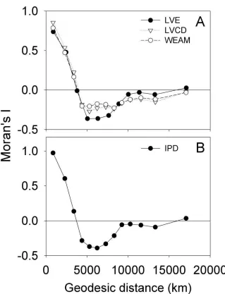
Recently, Gelade (2008) used spatial autocorrelation analysis to show that nations that are geographical neighbors have more similar mean IQs than nations that are far apart. One might equally find positive autocorrelation in candidate predictor variables of national mean IQ such as average temperature, or national per capita income T (1970) F L G everything else, but near things are more related than
5
another than to countries on different continents both in terms of national mean IQ and any number of potential predictors (e.g. disease burden as shown in Figure 1 and as hypothesised by Eppig et al., 2010). Additional statistical controls must be taken into account to explicitly deal with the spatial relationships among data points. Specifically, without controlling for autocorrelation, tests of association between spatially autocorrelated variables can lead to an inflated proportion of Type I errors (rejection of the null hypothesis when true), since the effective sample size is always smaller than the total number of genuinely independent data points (Clifford, Richardson, & Hemon, 1989; Legendre & Fortin, 1989; Legendre & Legendre, 1998). The problem may also be more severe than simply inflating Type I error rate. In particular, Lennon (2000) argued that correlations between an autocorrelated response variable and a set of candidate predictors will be strongly biased in favour of identifying autocorrelated predictors as significant over non-autocorrelated predictors.
While many papers have highlighted the problems posed by spatial autocorrelation in data, far fewer studies have offered a solution (Dale & Fortin, 2002). These solutions include discarding data, adjusting the Type I error rate, adjusting the effective sample size to control for lack of independence and accounting for spatial structure directly in the fitted model (Dale & Fortin, 2002). Whatever the remedy, one simply cannot ignore spatial autocorrelation and hope for the best (Beale, Lennon, Yearsley, Brewer, & Elston, 2010). Of course, it is quite possible for a spatially autocorrelated predictor to generate independent yet spatially autocorrelated responses when the response variable would not otherwise be autocorrelated. Using the example above, a positive correlation between national mean IQ and temperature would, by virtue of the spatial structure in temperature, produce a spatial structure in national IQ. Thus the two variables would be spatially autocorrelated but with an independent relationship. Therefore, conservatively controlling for spatial autocorrelation in predictor and response can throw the baby out with the bathwater and leave researchers with little additional variation to explain other than processes operating at different (usually smaller) spatial scales. Arguably therefore, controlling for a lack of spatial independence is only essential when the residuals of fitted models continue to show significant spatial signature (Diniz-Filho, Bini, & Hawkins, 2003) above and beyond those accounted for by the predictor, which will arise when the response continues to show a lack of independence even after controlling for Here we adopt this conservative approach in re-evaluating competing hypotheses to explain geographical patterns in national mean IQ. We show that spatial autocorrelation is present not only in the predictors of national mean IQ, but also in the residuals of models used to describe national IQ. The best fitting models exhibit greater explanatory power after control for spatial autocorrelation so, rather than obliterate any pattern, they remain capable of yielding insights into the question of how and why IQ varies across nations.
3. Competing hypotheses to explain geographical variation in mean IQ
Since Lynn and Vanhanen published their monographs on geographical variation in IQ (Lynn & Vanhanen, 2001), a number of competing hypotheses have emerged to explain variation between countries. We present a subset of representative hypotheses which can be classified using three broad categories:
6
Distance from the environment of evolutionary adaptedness (hereafter, "DEEA") (Kanazawa, 2008) Kanazawa proposed that the human brain was adapted to a particular ancestral environment: the savannah of central Africa. In order to exploit environments that differ from this habitat, the human brain would need to be able to adapt to solve new challenges. Kanazawa proposes that this requirement for greater intelligence is what selected for higher-IQ individuals in locations further from the environment of evolutionary adaptedness (EEA).
Temperature (Kanazawa, 2008; Templer & Arikawa, 2006) In a similar hypothesis, a variety of authors have suggested that cold weather and harsh winters select for higher intelligence to be able to cope with the extremes of climate.
Physiological hypotheses:
Nutrition (Lynn, 1990) Lynn observed that changes in height and head size were occurring over time. He hypothesised that this was the result of increasing levels of nutrition, citing evidence that nutritional deficiencies retard growth. Citing correlations between head size, brain size and IQ, Lynn then proposes that increases in nutrition are also increasing national mean IQ.
Parasite burden (Eppig, Fincher, & Thornhill, 2010) Significant international variation in IQ can be explained by variation in the disability-adjusted life years (DALY, a measure of disease burden) due to parasitic and infectious disease. The reasoning behind this hypothesis is that the response to parasites by the immune system requires energy which can then not be used in cognitive development.
Socioeconomic hypotheses:
Education (Barber, 2005) This hypothesis assumes that the amount of time put into education is related to the extent of cognitive development, which then influences IQ. Evidence for such a causal relationship has been presented using longitudinal studies (e.g. Richards & Sacker, 2003). Marks (2010) has argued that geographical variation in IQ is purely an artefact of literacy levels. However, literacy data are no longer collected in many high-income countries which are typically considered to be 99% literate (e.g. United Nations Development Programme, 2009). Here we assume that Marks' hypothesis based on literacy can be tested using data on education.
Gross domestic product (GDP) (Lynn & Vanhanen, 2002) GDP per capita is related to development which, in turn, is related to the average amount of education. For reasons described in the previous hypothesis, it might be expected that a higher general level of education would result in higher IQ.
All studies cited above have provided significant statistical results to support their hypotheses. However, none so far has either tested for or controlled for the spatial structure of the data in a rigorous way.
7
We begin by describing the sources for our data (which are provided in Appendix 1). We then demonstrate the extent of the spatial autocorrelation in the raw predictor and response variables. We show that strong correlations exist between all six candidate predictors and three measures of national mean IQ, even when spatial autocorrelation is taken into account. We use an exhaustive model selection method to find the most parsimonious model to explain variation in national mean IQ. Next, and most importantly, we show that the residuals of these best-fit multiple regression models exhibit spatial autocorrelation, which even by the least conservative standards necessitates the control of this autocorrelation in the analysis of the model (Diniz-Filho, et al., 2003). Finally, we then carry out the model selection procedure, this time including control for SAC.
Data sources
Data sources were used mostly as specified in Eppig et al. (2010): national IQ data were taken from Lynn and Vanhanen (2006) with 17 alternative values from Wicherts, Dolan, & van der Maas (2010); disability life-adjusted year (DALY) values for infectious and parasitic diseases (hereafter "IPD") and nutritional deficiencies ("Nut") were generated by the World Health Organisation (2004); average years in education ("AVED"), % population reaching enrolment in secondary education ("Sec_E") and % population completing secondary education ("Sec_C") from Barro & Lee (2010) and data at
http://www.barrolee.com/ for 2010; and GDP per capita ("GDP") from the CIA World Factbook (2007). Three IQ datasets were defined, as in Eppig et al: Lynn and Vanhanen's (2006) data based only on censuses ("LVCD"), Lynn and Vanhanen's data with estimates for missing values ("LVE") and LVE with the 17 alternative values from Wicherts, Dolan, & van der Maas (2010) ("WEAM"). Distance from the point 5°S, 25°E (the "environment of evolutionary adaptedness") to the centroid of each country ("DEEA") was calculated in ArcGIS v9.2 (ESRI, 2006). Centroids were also used in subsequent control for SAC. As an index of temperature, we calculated the mean temperature of the coldest quarter ("MTCQ") for each country using the WORLDCLIM dataset (Hijmans, Cameron, Parra, Jones, & Jarvis, 2005) in ArcGIS v9.2 (ESRI, 2006). Countries lacking any data were excluded leaving a total of 137 countries for the comparison (Table S1). IPD, Nut, GDP and DEEA were log-transformed for normality. The three education measures were highly collinear (Sec_E vs. Sec_C, r=0.942, p<0.001; Sec_E vs. AVED, r=0.935, p<0.001; Sec_C vs. AVED, r=0.892, p<0.001). Therefore, the three education variables were entered into a principal components analysis to produce a single education measure ("ED") from the first principal component which explained 97.7% of the variance in the three measures.
Data analysis
(i) SAC in predictors and responses
8
A distance matrix was first calculate based on great circle distances between each pair of country centroids using the "distCosine" function in the R package geosphere (Hijmans, Williams, & Vennes, 2011). Great circle distances take into account the curvature of the earth when calculating distances between two sets of latitude-longitude coordinates. The "Moran.I" function in the R package APE (Paradis, Claude, & Strimmer, 2004) was used to calculate the global Moran's I value for each of the nine variables. We have attached the R code for this operation in Appendix 2. To further illustrate the pattern of SAC in the data, the three IQ variables and IPD, highlighted as the most important predictor in a recent analysis (Eppig, et al., 2010) were analysed in SAM v4.0 (Rangel, Diniz-Filho, & Bini, 2006) over a range of distances. SAM ("Spatial Analysis in Macroecology") is free software available from
http://www.ecoevol.ufg.br/sam/. This software provides tools to carry out a variety of analyses including spatial eigenvector mapping, the quantification of SAC using Moran's I, and multimodel inference using A I C AIC).
(ii) Correlations between national mean IQ and predictors
Correlations between each of the predictors and the three national IQ indices were assessed using Pearson product-moment correlations (Table 2). Having previously demonstrated the presence of spatial autocorrelation in the predictors and response variables, it was clear that the degrees of freedom in the tests would be artificially inflated due to the lack of independence between data points. The "spatial correlation" function in SAM was used to recalculate the geographically effective degrees of freedom according to the method of Clifford et al. (1989). This allows a more accurate calculation of statistical significance.
(iii) First model construction
9
& Omland, 2004) A AIC AIC
of <2 indicates that there is substantial evidence for the given model above alternative candidate
models AIC AIC
(Burnham & Anderson, 2002). We also calculate R2 (the proportion of overall variance explained by the fitted model) as an absolute measure of goodness-of-fit to complement the relative measure provided by AICc. Six predictors yield a potential 63 models including a null model (with only a floating intercept) and each of these was constructed in R for each of the three IQ variables. The resulting models were compared using the "aictab" function in the AICcmodavg package (Mazerolle, 2010) in R. We have provided the R code for this stage of the analysis in Appendix 3.
(iv) SAC in model residuals
As stated above, the presence of SAC in model residuals indicates a need to account for SAC in the model itself. We tested for evidence of spatial autocorrelation in the best fitting models (for which
AIC IQ T M I R
described above, for the residuals of each of the models.
(v) Control for SAC
Having demonstrated that the residuals of the best fitting models exhibited spatial autocorrelation, the model selection procedure was carried out a second time with a control for SAC. The incorporation of SAC into these models was through a technique called "spatial eigenvector mapping" (SEVM) and was carried out in SAM. This method decomposes the spatial relationships between data into explanatory variables which capture spatial effects at different spatial resolutions. The method can be viewed as equivalent to a principal components analysis carried out on the distance matrix of the data (Dormann, et al., 2007). Whereas selection of relevant components in PCA hinges on their eigenvalues, we based selection of eigenvectors on the minimisation of Moran's I (to a threshold of 0.05) in the model residuals. The resulting eigenvectors are then included in all models during the model selection procedure. Global Moran's I was calculated for the residuals of each of the best fitting ( AIC
to evaluate the success of the method.
4. Results
(i) SAC in predictors and responses
10
distance from another given point. This near-tautological example of SAC is instructive in demonstrating the importance of accounting for lack of independence in analyses.
(ii) Correlations between national IQ and predictors
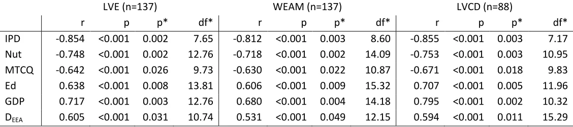
Before control for SAC, there were strong, significant (p<0.001 in all cases) correlations between all six predictor variables and the three national IQ measures (Table 2). The proportion of variance in the national IQ measures that was explained by the individual predictors range from 28% to 73%, with the strongest correlations between national IQ and IPD and the weakest between IQ and DEEA. When SAC was controlled for in these pairwise correlations there were still significant correlations at the reduced degrees of freedom. It is worth noting that the variables with higher SAC in Table 1 (IPD, DEEA and MTCQ) are those which have the greatest reduction in degrees of freedom in Table 2. However, this method still gives us no reason to choose between the competing hypotheses as all terms remain significant.
(iii) First model construction
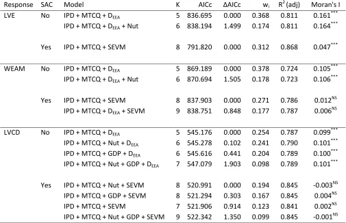
An exhaustive search of models prior to control for SAC yielded very similar models for each of the three national IQ measures (Table 3). In each of the LVE, WEAM and LVCD measures, IPD, MTCQ and DEEA
formed the top model and AIC N
second-ranking models in each case, and GDP featured in the third- and fourth-ranking models for LVCD. All models explain a large proportion of the variance in the response variables (between 72.3 and 81.1%).
(iv) SAC in model residuals
Examining the residuals for SAC we see that there is highly significant autocorrelation in the residuals of all the top models (Table 3). While this SAC is not as strong as that present in the raw data (Table 1), it provides strong evidence for a continuing effect of spatial interdependence in the models.
(v) Control for SAC
The inclusion of spatial eigenvectors in the model selection procedure, results in a change in our interpretation of the results. The first is that the explanatory power of all models increases (note the adjusted R2 values in Table 3). The lower AICc values demonstrate that this increase in goodness-of-fit does not come at a cost of decreased parsimony. In fact, the model fit according to AIC is substantially better after control for SAC, with AIC values comparing best-fit models before and after SAC of 44.875, 31.286 and 24.185 for LVE, WEAM and LVCD, respectively.
11
Third, the composition of the models changes. There is consistent evidence for an effect of IPD and MTCQ in the top models before controlling for SAC and this remains after the control is applied (Table 3). The most noticeable difference in model composition is the omission of DEEA (distance from the environment of evolutionary adaptedness) from most of the models after control for SAC. Having been present in all top models prior to control for SAC, DEEA occurs only once in the second-best fit model for the WEAM IQ measure. Nut also seems to increase in importance but only in the LVCD IQ measure, where GDP also remains in the best-fit models.
5. Discussion
We have highlighted the importance of dealing with spatial autocorrelation when analysing spatial patterns, and re-examined competing hypotheses explaining geographical variation in national IQ to illustrate our case. Cross-national research in mean IQ is a relatively new field but has already produced a number of studies which have sought predictors of variation in IQ. Such putative predictors have included temperature and skin colour (Templer & Arikawa, 2006), evolutionary novelty (Kanazawa, 2008), irreligion (Lynn, Harvey, & Nyborg, 2009), inbreeding (Woodley, 2009) and a range of economic factors (e.g. Dickerson, 2006). While these studies may provide interesting results, none have explicitly considered spatial autocorrelation. It has long been appreciated (e.g. Clifford, et al., 1989) that not accounting for spatial autocorrelation in the response variable results in inflated significance due to overestimation of the true sample size of data. While this is true for any spatial analysis, different fields have taken different lengths of time to address the problem. Geography was among the first (Cliff & Ord, 1970), with ecology following later (Legendre, 1993) and other subdisciplines of biology only now incorporating the issues into their paradigms (Valcu & Kempenaers, 2010). In this paper we highlight the issue of spatial autocorrelation in the context of spatial variation in intelligence.
Correcting for SAC in conjunction with exhaustive model selection enables us to circumvent the twin problems of spatial autocorrelation and collinearity among variables. This permits the most comprehensive and statistically rigorous assessment of six potential hypotheses explaining variation in geographical patterns in IQ that has yet been conducted. When a comprehensive model comparison was conducted to analyse national variation in IQ scores, then infectious and parasitic diseases (IPD) and temperature (mean temperature of the coldest quarter) were the only two variables consistently included in models. Mortality and morbidity resulting from nutritional deficiencies (Nut), GDP, and distance from the environment of evolutionary adaptedness (DEEA) also feature in some of the best fitting models. However, it is worth noting that DEEA becomes far less important in models after controlling for SAC. This is not surprising given that the variable itself is, by definition, autocorrelated across space. It seems likely that the distance from the environment of evolutionary adaptedness has no causal link with national mean IQ.
12
the interaction between humans and their diseases. Temperature influences a number of disease-related parameters such as disease distribution (Guernier, Hochberg, & Guégan, 2004), transmission seasons (e.g. malaria, Hay, Guerra, Tatem, Noor, & Snow, 2004), the ability of insect vectors to transmit diseases (Cornel, Jupp, & Blackburn, 1993) and the development and survival of parasites and host susceptibility (Harvell, et al., 2002). It may be that temperature is having an effect on national mean IQ by mediating the response to infectious diseases rather than via environmental complexity.
We have highlighted SAC as a cause for concern in these analyses of geographic variation in IQ and briefly mentioned multicollinearity in the predictor variables as a second issue. While we use exhaustive (or "all-subsets") modelling to avoid issues with collinear predictor variables and model construction, an alternative method would be structural equation modelling (SEM, or "path analysis") (Graham, 2003); (van der Maas, et al., 2006). SEM involves the explicit, a priori statement of causal and correlative relationships between variables and provides estimates of the relative strengths of interactions. Where, for example, changes in sanitation are thought to cause changes in disease, or changes in nutrition cause changes in infant mortality, these effects can be stated and the direct and indirect effects on national IQ can be assessed. While this approach shows promise for testing hypotheses of national IQ variation, there are cases in which the nature of relationships are unclear. For example, does GDP exert a causal relationship on other factors? Does education improve nutrition and/or disease incidence?
Socioeconomic factors do not feature strongly in the analysis when other factors are taken into account. GDP is present in some of the best-fitting models but it is unclear as to how this variable is acting. There has been debate in the literature over the competence of IQ tests to accurately measure intelligence over a range of education or literacy levels (Barber, 2005), with some researchers claiming that global variation in IQ is entirely an artefact of varying literacy (Marks, 2010). We find no evidence to support this. However, we stress that our measure of education, despite being a composite statistic will not have captured all aspects of educational experience, so as always, alternative measures could have given different results. Intriguingly, cross-fostering studies have demonstrated that socio-economic factors can influence IQ, with children from high socioeconomic status (SES) parents who were subsequently fostered by low SES parents having lower IQ scores than those children from high SES families who were then fostered by other high SES parents. Conversely, children from low SES parents who were fostered by high SES foster parents exhibited higher IQ scores than did children from low SES parents who were fostered by low SES foster parents (Capron & Duyme, 1989). It is worth noting that this study was conducted only in France, and so the results may not be applicable to a global study with far greater variations in SES. It may be that SES acts at a smaller scale that is dwarfed by other factors on a global level.
13
end of the IQ distribution (Colom, Lluis-Font, & Andrés-Pueyo, 2005). Parasites in host populations commonly exhibit aggregation, with a few individuals carrying large numbers of parasites and most individuals carrying few (Anderson & Gordon, 1982). It could be reasoned that either improved hygiene or clinical intervention for diseases and parasites is benefitting those few heavily infected individuals disproportionately and, if those individuals also exhibit low IQ as a result of their disease burden, IQ would also increase to the greatest extent at the lower end of the scale. Thus, a parasite-induced depression in IQ with subsequent improvement due to hygiene and medicine could provide an explanation for the Flynn Effect (Eppig, et al., 2010).
Controlling for autocorrelation may remove real biological patterns and this has been offered as an argument against controlling for both spatial (Legendre, 1993) and phylogenetic (Ricklefs & Starck, 1996) autocorrelation. However, any statistical analysis with an inherent spatial component should consider spatial autocorrelation, if only to demonstrate that its control is not necessary. Failure to account for this lack of independence in data violates statistical assumptions and renders statistical inference invalid. The initial dogmatism with which controls for spatial and phylogenetic autocorrelation were enforced has now given way to an acceptance that such controls are not always necessary. However, with the advent of numerous tools and techniques (such as those presented here) for assessing this need, we encourage researchers to at least give the topic due consideration as it can substantially influence results.
Acknowledgements
We would like to thank the Carleton University ECO-EVO Group for discussion. Conor Dolan, Douglas Detterman, Jelte Wicherts and an anonymous referee provided comments which greatly improved the manuscript. CH was supported by an Ontario Ministry of Research and Innovation Postdoctoral Fellowship and TNS is funded by NSERC.
References
Anderson, R. M., & Gordon, D. M. (1982). Processes influencing the distribution of parasite numbers within host populations with special emphasis on parasite-induced host mortalities. Parasitology, 85, 373-398.
Barber, N. (2005). Educational and ecological correlates of IQ: A cross-national investigation. Intelligence, 33, 273-284.
Barro, R. J., & Lee, J.-W. (2010). A new data set of educational attainment in the world, 1950-2010 (Vol. 15902). Cambridge, USA: National Bureau of Economic Research.
Beale, C. M., Lennon, J. J., Yearsley, J. M., Brewer, M. J., & Elston, D. A. (2010). Regression analysis of spatial data. Ecology Letters, 13, 246-264.
Burnham, K. P., & Anderson, D. R. (2002). Model Selection and Multimodel Inference: A Practical Information-Theoretic Approach (2nd ed.). New York: Springer-Verlag.
Capron, C., & Duyme, M. (1989). Assessment of effects of socio-economic status on IQ in a full cross-fostering study. Nature, 340, 552-553.
14
Cliff, A. D., & Ord, K. (1970). Spatial autocorrelation: a review of existing and new measures with applications. Economic Geography, 46, 269-292.
Clifford, P., Richardson, S., & Hemon, D. (1989). Assessing the significance of the correlation between two spatial processes. Biometrics, 45, 123-134.
Colom, R., Lluis-Font, J. M., & Andrés-Pueyo, A. (2005). The generational intelligence gains are caused by decreasing variance in the lower half of the distribution: Supporting evidence for the nutrition hypothesis. Intelligence, 33, 83-91.
Cornel, A. J., Jupp, P. G., & Blackburn, N. K. (1993). Environmental temperature on the vector competence of Culex univittatus (Diptera: Culicidae) for West Nile Virus. Journal of Medical Entomology, 30, 449-456.
Dale, M. R. T., & Fortin, M.-J. (2002). Spatial autocorrelation and statistical tests in ecology. Ecoscience, 9, 162-167.
Dickerson, R. E. (2006). Exponential correlation of IQ and the wealth of nations. Intelligence, 34, 291-295.
Diniz-Filho, J. A. F., Bini, L. M., & Hawkins, B. A. (2003). Spatial autocorrelation and red herrings in geographical ecology. Global Ecology and Biogeography, 12, 53-64.
Dormann, C. F., McPherson, J. M., Araújo, M. B., Bivand, R., Bolliger, J., Carl, G., Davies, R. G., Hirzel, A., Jetz, W., Daniel Kissling, W., Kühn, I., Ohlemüller, R., Peres-Neto, P. R., Reineking, B., Schröder, B., Schurr, F. M., & Wilson, R. (2007). Methods to account for spatial autocorrelation in the analysis of species distributional data: a review. Ecography, 30, 609-628.
Duckworth, A. L., Quinn, P. D., Lynam, D. R., Loeber, R., & Stouthamer-Loeber, M. (in press). Role of test motivation in intelligence testing. Proceedings of the National Academy of Sciences.
Eppig, C., Fincher, C. L., & Thornhill, R. (2010). Parasite prevalence and the worldwide distribution of cognitive ability. Proceedings of the Royal Society: Series B (Biological Sciences), First cite, doi:10.1098/rspb.2010.0973.
ESRI. (2006). ArcGIS v.9.2. Redlands: Environmental Systems Research Institute, Inc. Gelade, G. A. (2008). The geography of IQ. Intelligence, 36, 495-501.
Gould, S. J. (1981). The Mismeasure of Man. New York: W.W. Norton & Co.
Graham, M. (2003). Confronting multicollinearity in ecological multiple regression. Ecology, 84, 2809-2815.
Guernier, V., Hochberg, M. E., & Guégan, J.-F. (2004). Ecology drives the worldwide distribution of human diseases. PLoS Biology, 2, e141.
Harvell, C. D., Mitchell, C. E., Ward, J. R., Altizer, S., Dobson, A. P., Ostfeld, R. S., & Samuel, M. D. (2002). Climate warming and disease risks for terrestrial and marine biota. Science, 296, 2158-2162. Hay, S. I., Guerra, C. A., Tatem, A. J., Noor, A. M., & Snow, R. W. (2004). The global distribution and
population at risk of malaria: past, present and future. Lancet Infectious Diseases, 4, 327-336. Hijmans, R. J., Cameron, S. E., Parra, J. L., Jones, P. G., & Jarvis, A. (2005). Very high resolution
interpolated climate surfaces for global land areas. International Journal of Climatology, 25, 1965-1978.
15
Hunt, E., & Carlson, J. (2007). Considerations relating to the study of group differences in intelligence. Perspectives on Psychological Science, 2, 194-213.
Jensen, A. R. (1982). The debunking of scientific fossils and straw persons. Contemporary Education Review, 1, 121-135.
Johnson, J. B., & Omland, K. S. (2004). Model selection in ecology and evolution. Trends in Ecology & Evolution, 19, 101-108.
Kanazawa, S. (2008). Temperature and evolutionary novelty as forces behind the evolution of general intelligence. Intelligence, 36, 99-108.
Kutner, M., Nachtsheim, C., Neter, J., & Li, W. (2005). Applied Linear Statistical Models (5th ed.). Irwin, CA: McGraw-Hill.
Legendre, P. (1993). Spatial autocorrelation: trouble or new paradigm? Ecology, 74, 1659-1673. Legendre, P., & Fortin, M.-J. (1989). Spatial pattern and ecological analysis. Vegetatio, 80, 107-138. Legendre, P., & Legendre, L. (1998). Numerical Ecology. Amsterdam: Elsevier Science.
Lynn, R. (1990). The role of nutrition in secular increases in intelligence. Personality and Individual Differences, 11, 273-285.
Lynn, R., Harvey, J., & Nyborg, H. (2009). Average intelligence predicts atheism rates across 137 countries. Intelligence, 37, 11-15.
Lynn, R., & Vanhanen, T. (2001). National IQ and economic development: a study of eighty-one nations. Mankind Quarterly, 41, 415-435.
Lynn, R., & Vanhanen, T. (2002). IQ and the Wealth of Nations. Westport, CT: Praeger. Lynn, R., & Vanhanen, T. (2006). IQ and global inequality. Augusta, GA: Washington Summit.
Marks, D. F. (2010). IQ variations across time, race and nationality: an artifact of differences in literary skills. Psychological Reports, 106, 643-664.
Mazerolle, M. J. (2010). AICcmodavg: model selection and multimodel inference based on (Q)AIC(c). R package version 1.13: http://CRAN.R-project.org/package=AICcmodavg.
Paradis, E., Claude, J., & Strimmer, K. (2004). APE: analyses of phylogenetics and evolution in R language. Bioinformatics, 20, 289-290.
Rangel, T. F. L. V. B., Diniz-Filho, J. A. F., & Bini, L. M. (2006). Towards an intergrated computational tool for spatial analysis in macroecology and biogeography. Global Ecology and Biogeography, 15, 321-327.
Richards, M., & Sacker, A. (2003). Life course antecedents of cognitive reserve. Journal of Clinical Experimental Neuropsychology, 25, 614-624.
Ricklefs, R. E., & Starck, J. M. (1996). Applications of phylogenetically independent contrasts: a mixed progress report. Oikos, 77, 167-172.
Sokal, R. R., & Oden, N. L. (1978). Spatial autocorrelation in biology 1. Methodology. Biological Journal of the Linnaean Society, 10, 199-228.
Templer, D. I., & Arikawa, H. (2006). Temperature, skin color, per capita income, and IQ: An international perspective. Intelligence, 34, 121-139.
Tobler, W. (1970). A computer movie simulating urban growth in the Detroit region. Economic Geography, 46, 234-240.
16
Valcu, M., & Kempenaers, B. (2010). Spatial autocorrelation: an overlooked concept in behavioral ecology. Behavioral Ecology, 21, 902-905.
van der Maas, H. L. J., Dolan, C. V., Grasman, R. P. P. P., Wicherts, J. M., Huizenga, H. M., & Raijmakers, M. E. J. (2006). A dynamical model of general intelligence: the positive manifold of intelligence by mutualism. Psychological Review, 113, 842-861.
WHO. (2004). Global burden of disease: 2004 update. Geneva, Switzerland: World Health Organisation. Wicherts, J. M., Borsboom, D., & Dolan, C. V. (2010). Why national IQs do not support evolutionary
theories of intelligence. Personality and Individual Differences, 48, 91-96.
Wicherts, J. M., Dolan, C. V., Carlson, J. S., & van der Maas, H. L. J. (2010). Raven's test performance of sub-Saharan Africans: mean level, psychometric propoerties and the Flynn Effect. Learning and Individual Differences, 20, 135-151.
Wicherts, J. M., Dolan, C. V., Hessen, D. J., Oosterveld, P., van Baal, G. C. M., Boomsma, D. I., & Span, M. M. (2004). Are intelligence tests measurement invariant over time? Investigating the nature of the Flynn effect. Intelligence, 32, 509-537.
Wicherts, J. M., Dolan, C. V., & van der Maas, H. L. J. (2010). A systematic literature review of the average IQ of sub-Saharan Africans. Intelligence, 38, 1-20.
Woodley, M. A. (2009). Inbreeding depression and IQ in a study of 72 countries. Intelligence, 37, 268-276.
17 Tables
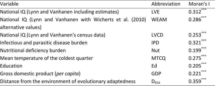
Table 1 Three measures of national IQ and six predictor variables with the extent of spatial autocorrelation (global Moran's I). Each of these variables exhibit highly significant (denoted ***) spatial structuring, in that we can readily reject the null hypothesis of no spatial structure (p<0.001). N=137, except for LVCD where N=88.
Variable Abbreviation Moran's I
National IQ (Lynn and Vanhanen including estimates) LVE 0.312*** National IQ (Lynn and Vanhanen with Wicherts et al. (2010)
alternative values)
WEAM 0.286***
National IQ (Lynn and Vanhanen's census data) LVCD 0.253*** Infectious and parasitic disease burden IPD 0.321***
Nutritional deficiency burden Nut 0.199***
Mean temperature of the coldest quarter MTCQ 0.275***
Education Ed 0.205***
[image:18.612.72.501.149.321.2]18
Table 2 Product moment coefficients and significance of correlations between three national IQ measures (see text for details) and eight putative predictors (see text for definitions) before (r and p) and after (p*=corrected p-value, df*=estimated corrected degrees of freedom) control for spatial autocorrelation. Degrees of freedom prior to correlation for autocorrelation are 135 for LVE and WEAM and 85 for LVCD.
LVE (n=137) WEAM (n=137) LVCD (n=88)
r p p* df* r p p* df* r p p* df*
[image:19.612.30.594.165.290.2]19
Table 3 Model selection table for exploratory analysis before (SAC is "no") and after (SAC is "yes") control for spatial autocorrelation. For definitions of model terms see text and Table 1. Significance of Moran's I is indicated by: ***=p<0.001, NS=p>0.05. Note that after control for SAC, Moran's I for the model explaining LVE is still significant. This is due to the SEVM routine acting to reduce the magnitude of SAC below a specific threshold (0.05), rather than reducing the significance of the pattern.
Response SAC Model K AICc AIC wi R2 (adj) Moran's I
LVE No IPD + MTCQ + DEEA 5 836.695 0.000 0.368 0.811 0.161*** IPD + MTCQ + DEEA + Nut 6 838.194 1.499 0.174 0.811 0.164***
Yes IPD + MTCQ + SEVM 8 791.820 0.000 0.312 0.868 0.047***
WEAM No IPD + MTCQ + DEEA 5 869.189 0.000 0.378 0.724 0.105*** IPD + MTCQ + DEEA + Nut 6 870.694 1.505 0.178 0.723 0.106***
Yes IPD + MTCQ + SEVM 8 837.903 0.000 0.271 0.786 0.012NS IPD + MTCQ + DEEA + SEVM 9 838.751 0.848 0.177 0.787 0.006NS
LVCD No IPD + MTCQ + DEEA 5 545.176 0.000 0.254 0.787 0.099*** IPD + MTCQ + Nut + DEEA 6 545.278 0.102 0.241 0.790 0.101*** IPD + MTCQ + GDP + DEEA 6 545.616 0.441 0.204 0.789 0.100*** IPD + MTCQ + Nut + GDP + DEEA 7 547.079 1.903 0.098 0.789 0.101***
[image:20.612.71.576.150.476.2]20 Figure legends
21
[image:22.612.147.466.82.499.2]22
Appendix 1 Raw data
Country/Region LVE LVCD WEAM IPD Nut WMH MTCQ Sec_E Sec_C AVED GDP DEEA Long (°E) Lat (°N)
Afghanistan 84 -- 84 12010.86 1515.57 8 -0.22 32 20 3.33 1000 6099.23 66.024 33.841
Albania 90 -- 90 488.65 620.97 13 3.60 121.7 43.2 10.38 6400 5155.07 20.081 41.141
Algeria 83 -- 83 1974.29 439.38 17 13.14 81.5 47.2 7.04 7100 4397.88 2.630 28.159
Andorra 98 -- 98 274.39 76.91 -- -2.40 -- -- -- 44900 5790.11 1.578 42.533
Angola 68 -- 68 19078.39 2142.56 23 18.79 -- -- -- 8400 1154.33 17.541 -12.312
Antigua and Barbuda 70 -- 70 953.56 196.59 -- 24.85 -- -- -- 17800 9833.34 -61.788 17.316
Argentina 93 93 93 836.38 175.63 -- 8.00 90.1 45 9.28 13400 9702.72 -65.188 -35.401
Armenia 94 -- 94 1003.55 171.94 2 -4.49 171.8 97.2 10.79 5500 5433.52 44.939 40.301
Australia 98 98 98 155.27 36.39 -- 14.72 157 94.7 12.04 40000 11693.66 134.493 -25.744
Austria 100 100 100 188.31 78.77 0 -3.20 131.6 69.6 9.77 39200 5943.62 14.151 47.591
Azerbaijan 87 -- 87 1993.68 509.98 3 1.51 -- -- -- 10400 5535.39 47.540 40.269
Bahrain 83 -- 83 546.60 247.13 20 17.90 129.8 63.5 9.42 38800 4415.61 50.574 26.020
Bangladesh 82 -- 82 4959.85 716.59 26 19.84 56.4 25.7 4.77 1500 7757.80 90.263 23.895
Barbados 80 80 80 1371.81 122.77 -- 24.20 114 27.6 9.34 17700 9544.84 -59.531 13.184
Belarus 97 -- 97 664.02 354.60 5 -5.34 -- -- -- 12500 6515.06 28.051 53.535
Belgium 99 99 99 173.03 76.16 4 2.34 131.4 79.6 10.57 36800 6485.28 4.669 50.633
Belize 84 -- 84 1615.56 404.98 -- 22.60 53.1 27.6 9.18 8300 12687.09 -88.699 17.169
Benin 70 -- 70 10870.93 1143.10 27 25.21 33.2 17.5 3.25 1500 2991.75 2.338 9.628
Bermuda 90 90 90 -- -- -- 3.11 -- -- -- 69900 10281.90 -64.760 32.305
Bhutan 80 -- 80 4542.08 861.62 10 17.50 -- -- -- 4700 7882.89 90.443 27.425
Bolivia 87 87 87 3401.17 796.83 -- 0.25 106.2 62.4 9.20 4700 9812.51 -64.667 -16.713
Bosnia and Herzegovina 90 -- 90 286.73 358.41 -- 14.64 -- -- -- 6400 5514.50 17.789 44.167
Botswana 70 -- 70 32483.12 532.08 24 3.90 107 35.7 8.90 12800 1915.18 23.806 -22.185
Brazil 87 87 87 1575.02 363.48 -- 22.95 77.9 37.6 7.18 10100 8606.73 -53.100 -10.784
Brunei 91 -- 91 655.77 146.07 30 26.52 99.1 45.1 8.57 51200 10018.49 114.702 4.534
Bulgaria 93 93 93 300.30 352.63 4 0.43 109.5 57.4 9.95 12500 5310.37 25.249 42.757
Burkina Faso 68 -- 68 15706.29 1405.28 33 25.61 -- -- -- 1200 3526.84 -1.765 12.265
Burundi 69 -- 69 18706.93 1439.56 29 18.92 11.1 4.9 2.69 300 578.49 29.942 -3.336
Cambodia 91 -- 91 8687.43 1238.76 31 24.85 24.1 9.3 5.77 1900 9045.27 104.946 12.718
Cameroon 64 64 64 16696.47 821.09 30 23.07 43.2 17.7 5.91 2300 1805.84 12.759 5.693
Canada 99 99 99 183.10 62.08 -- -23.33 147.3 83.6 11.49 38200 12214.43 -98.348 61.290
Cape Verde 76 -- 76 3558.65 520.18 -- 19.38 -- -- -- 3600 5868.58 -23.931 16.039
Central African Republic 64 64 71 20453.29 922.71 32 23.66 27.7 11.7 3.54 700 1380.58 20.491 6.571
Chad 68 -- 68 18199.74 1104.79 32 21.97 -- -- -- 1900 2366.71 18.672 15.341
Chile 90 90 90 491.35 122.76 -- 4.80 109.8 66.8 9.74 14600 10224.69 -71.293 -37.287
China 105 105 105 985.88 252.96 7 -7.02 106.9 50.4 7.55 6600 9350.61 103.841 36.567
Colombia 84 84 84 1167.21 228.23 -- 23.79 88.1 49.7 7.34 9200 10937.90 -73.073 3.903
Comoros 77 -- 77 5218.65 868.15 -- 20.50 -- -- -- 1000 2206.53 43.801 -11.965
Cook Islands 89 89 89 1613.48 272.12 -- 21.80 -- -- -- 9100 17127.24 -158.998 -20.673
23
Côte d'Ivoire 69 -- 69 21244.21 900.05 31 24.81 30.4 12.8 3.31 1700 3669.27 -5.557 7.628
Croatia 90 90 90 167.40 102.71 12 1.62 99.3 42.5 8.98 17500 5633.15 16.413 45.073
Cuba 85 85 85 454.12 201.51 -- 22.35 120 51.8 10.20 9700 11654.51 -78.967 21.587
Cyprus 91 -- 91 385.54 88.89 16 10.57 119 75.2 9.75 21000 4541.20 33.277 35.090
Czech Republic 98 98 98 131.48 104.19 1 -1.85 157.3 81.3 12.32 24900 6156.59 15.377 49.734 Democratic Republic of the Congo 64 64 75.9 18840.98 1151.02 27 23.01 35.7 13.7 3.47 300 279.35 23.657 -2.875
Denmark 98 98 98 162.10 70.94 3 0.37 101.3 58.1 10.27 36000 6919.03 10.010 55.989
Djibouti 68 -- 68 10816.33 705.65 29 23.32 -- -- -- 2700 2688.32 42.551 11.726
Dominica 67 67 67 950.01 149.43 -- 22.80 -- -- -- 10200 9766.43 -61.356 15.430
Dominican Republic 82 82 82 2897.34 347.07 -- 22.09 58.5 30.2 6.91 8300 10764.20 -70.493 18.933
East Timor 87 -- 87 8065.04 746.23 -- -- -- -- -- 2400 -- -- --
Ecuador 88 88 88 1764.69 355.49 -- 20.16 71.6 43.7 7.59 7500 11510.93 -78.706 -1.432
Egypt 81 81 81 1208.84 378.90 20 13.89 79.7 37.9 6.40 6000 3542.55 29.868 26.508
El Salvador 80 -- 80 2044.62 457.71 -- 23.24 69.1 36.8 7.54 7200 12711.49 -88.837 13.733
Equatorial Guinea 59 59 59 17396.06 972.55 31 21.93 -- -- -- 37500 1788.14 10.366 1.699
Eritrea 68 -- 85 7081.69 730.49 26 22.98 -- -- -- 700 2728.59 38.856 15.342
Estonia 99 99 99 537.88 178.28 4 -5.45 160.7 93.9 12.01 18500 7082.46 25.585 58.692
Ethiopia 64 64 69.4 14752.42 1487.59 24 21.21 -- -- -- 900 2219.29 39.632 8.618
Federated States of Micronesia 84 -- 84 1801.25 341.85 -- 26.10 -- -- -- 2200 14946.08 159.192 6.568
Fiji 85 85 85 1766.66 1212.72 -- 22.35 155.9 80.7 11.04 3900 15803.90 174.124 -17.474
Finland 99 99 99 124.36 71.95 5 -10.33 109.6 66.9 10.29 34100 7731.33 26.268 64.523
France 98 98 98 224.51 64.15 8 3.35 132.7 72 10.43 32600 6145.07 2.542 46.556
Gabon 64 -- 64 12506.99 440.29 28 22.91 69.5 37.3 7.50 14000 1545.46 11.796 -0.604
Georgia 94 -- 94 1099.73 341.79 7 -1.57 -- -- -- 4400 5570.18 43.535 42.170
Germany 99 99 99 173.31 70.47 2 0.14 160.2 87.5 12.21 34100 6391.60 10.401 51.098
Ghana 71 71 73.3 11517.62 554.42 33 25.24 76.2 19.3 7.09 1500 3245.01 -1.224 7.937
Greece 92 92 92 153.65 74.16 11 5.75 122.8 78.9 10.50 31000 4905.96 22.867 39.076
Grenada 71 -- 71 1347.46 313.44 -- -- -- -- -- 10300 9762.71 -61.659 12.145
Guatemala 79 79 79 2383.29 712.70 -- 21.05 30 14.8 4.07 5100 12870.04 -90.359 15.684
Guinea 67 67 67 11303.92 943.06 31 23.92 -- -- -- 1000 4331.22 -10.924 10.412
Guinea-Bissau 67 -- 67 15144.15 1411.63 29 24.70 -- -- -- 1100 4802.78 -14.914 12.051
Guyana 87 -- 87 4231.33 588.69 -- 25.31 66.8 29.6 7.96 6500 9390.28 -58.986 4.790
Haiti 67 -- 67 10121.21 1808.30 -- 22.18 52.3 24.2 4.90 1300 10995.20 -72.691 18.947
Honduras 81 81 81 2503.42 646.62 -- 21.72 51.5 23.7 6.50 4100 12472.03 -86.628 14.824
Hong Kong 108 108 108 -- -- 18 -- 111.6 58.7 10.02 42800 -- -- --
Hungary 98 98 98 234.23 191.62 1 -0.11 159.6 78.6 11.67 18800 5826.80 19.426 47.170
Iceland 101 101 101 156.63 65.13 2 -3.22 101.6 67.3 10.41 39600 8553.61 -18.565 64.986
India 86 86 86 4753.22 798.66 19 17.66 43.4 10.6 4.40 3100 6689.39 79.606 22.901
Indonesia 87 87 87 3099.10 534.30 30 24.44 51.3 26.2 5.82 4000 10240.12 117.299 -2.262
Iran 84 84 84 945.47 412.24 13 6.26 92.6 55.6 7.25 12500 5197.54 54.305 32.559
Iraq 87 87 87 3589.48 1247.97 17 9.90 50.8 28.1 5.56 3800 4672.31 43.765 33.066
Ireland 92 92 92 154.21 80.40 8 4.87 134.3 83 11.61 41000 7174.64 -8.144 53.178
24
Italy 102 102 102 193.46 93.81 11 4.42 112.2 49.1 9.30 29900 5469.60 12.100 42.777
Jamaica 71 71 71 2009.08 235.95 -- 22.59 113 55.4 9.63 8400 11479.68 -77.313 18.155
Japan 105 105 105 164.38 121.96 5 -0.17 135.2 90.2 11.48 32700 12371.04 138.082 37.630
Jordan 84 84 84 659.38 414.30 12 9.17 110.5 63 8.65 5200 4217.21 36.754 31.229
Kazakhstan 94 -- 94 1773.43 447.08 7 -11.24 145.4 70.2 10.37 11800 7198.73 67.283 48.156
Kenya 72 72 80.4 20742.34 648.00 25 22.81 32 5.8 6.95 1600 1553.54 37.853 0.511
Kiribati 85 -- 85 2831.69 958.37 -- -- -- -- -- 6100 19575.96 -157.381 1.846
Kuwait 86 86 86 347.74 147.28 16 13.32 70.2 30.6 6.10 52800 4514.29 47.571 29.329
Kyrgyzstan 90 -- 90 1919.37 395.93 1 -13.14 125.9 57.8 9.27 2200 7203.28 74.597 41.473
Laos 89 89 89 5878.70 1335.93 28 19.01 38.6 13.7 4.58 2100 9007.13 103.767 18.494
Latvia 98 -- 98 484.91 185.92 4 -4.89 148.2 71.2 10.42 14400 6875.93 24.933 56.837
Lebanon 82 82 82 845.15 232.97 14 7.40 -- -- -- 13200 4474.79 35.876 33.907
Lesotho 67 -- 67 32692.74 791.27 16 5.83 34.9 13.5 5.78 1600 2754.93 28.225 -29.587
Liberia 67 -- 67 18575.71 1592.94 30 24.54 38.4 20 3.93 400 4014.22 -9.304 6.428
Libya 83 -- 83 974.18 329.67 17 13.02 76.1 43 7.26 13400 3640.01 18.021 27.032
Lithuania 91 91 91 394.24 403.27 5 -4.28 165.6 97.4 10.91 15500 6708.79 23.890 55.327
Luxembourg 100 -- 100 194.83 84.20 3 1.38 114.2 60.7 10.09 79600 6355.57 6.120 49.763
Madagascar 82 82 82 7071.54 1010.55 -- 19.70 -- -- -- 1000 2843.71 46.712 -19.372
Malawi 69 -- 69 28720.38 1490.11 23 18.64 23.6 8.6 4.24 800 1367.06 34.288 -13.197
Malaysia 92 92 92 1754.50 348.67 29 24.93 108.2 52.7 9.53 14900 9461.21 109.723 3.800
Maldives 81 -- 81 2096.54 560.42 -- -- 47.5 14.4 4.74 4300 5450.07 73.298 3.629
Mali 69 -- 74.1 16123.99 1824.26 32 22.10 8.9 4.8 1.38 1200 3998.16 -3.525 17.348
Malta 97 97 97 203.19 79.23 -- 12.40 89.9 31.6 9.93 24300 4676.29 14.455 35.875
Marshall Islands 84 84 84 3032.30 517.28 -- -- -- -- -- 2500 15945.34 168.291 8.364
Mauritania 76 -- 76 8766.12 841.17 29 20.75 22.1 10.2 3.74 2000 4772.86 -10.332 20.257
Mauritius 89 89 89 1027.27 247.19 -- 19.40 73.8 28.1 7.18 13000 3931.62 57.819 -20.265
Mexico 90 90 90 787.46 240.87 -- 15.31 90.3 48.4 8.52 13200 14026.68 -102.516 23.943
Moldova 96 -- 96 803.91 514.09 1 -2.10 137.4 60.1 9.68 2300 5812.95 28.494 47.186
Monaco -- -- -- 240.78 57.01 -- 6.60 -- -- -- 30000 5700.06 7.419 43.748
Mongolia 101 -- 101 1955.47 250.38 19 -18.35 130 60.1 8.31 3100 9513.05 103.051 46.831
Morocco 84 84 84 1336.15 553.12 18 9.75 44 25.3 4.37 4700 5274.83 -6.326 31.900
Mozambique 64 64 64 20148.13 1075.78 26 20.49 5.5 2.4 1.21 900 1782.92 35.529 -17.282
Myanmar 87 -- 87 6649.77 939.78 28 18.70 30.8 19.5 3.97 1100 8312.78 96.520 21.197
Namibia 70 -- 74 19094.46 664.94 21 14.78 74 29.9 7.37 6600 2082.17 17.236 -22.152
Nauru -- -- -- 3216.93 400.25 -- -- -- -- -- 5000 15741.83 166.924 -0.527
Nepal 78 78 78 5467.80 1219.41 18 7.28 36.7 11.5 3.24 1200 7305.85 83.942 28.252
Netherlands 100 100 100 174.44 78.51 5 2.46 144.7 81.8 11.17 39500 6625.59 5.635 52.265
New Caledonia 85 85 85 -- -- -- 18.81 -- -- -- 15000 14821.87 165.624 -21.305
New Zealand 99 99 99 144.22 28.92 -- 5.46 112.8 89.4 12.51 27400 13827.31 171.916 -41.788
Nicaragua 81 -- 81 1498.59 476.38 -- 23.87 59.3 37.6 5.77 2800 12300.08 -85.035 12.837
Niger 69 -- 69 19113.87 1612.52 34 20.36 7.9 3.9 1.44 700 3024.05 9.412 17.421
Nigeria 69 69 83.8 17976.10 835.71 31 24.21 -- -- -- 2300 2478.12 8.107 9.605
25
North Korea 106 -- 106 2859.10 653.64 1 -9.21 -- -- -- 1900 11402.46 127.206 40.140
Northern Mariana Islands 81 81 81 -- -- -- -- -- -- -- 12500 13443.99 145.691 15.097
Norway 100 100 100 138.12 59.58 2 -7.36 159.5 88.4 12.63 57400 7766.91 14.041 64.369
Oman 83 -- 83 556.23 284.78 25 20.51 -- -- -- 25000 4432.51 56.109 20.621
Pakistan 84 84 84 4503.59 575.07 20 9.82 59.7 30.6 4.87 2500 6117.79 69.384 29.957
Palau -- -- -- 1975.90 334.69 -- -- -- -- -- 8100 12238.51 134.619 7.579
Panama 84 -- 84 1445.01 316.40 -- 24.40 103.1 63.7 9.39 12100 11750.23 -80.134 8.528
Papua New Guinea 83 83 83 6463.42 1380.44 -- 22.83 28.5 11.1 4.34 2300 13254.52 145.184 -6.465
Paraguay 84 84 84 1468.57 691.77 -- 18.91 81.4 37.5 7.70 4600 9114.62 -58.394 -23.231
Peru 85 85 85 2052.19 513.03 -- 17.88 112.1 65.9 8.66 8500 10943.62 -74.380 -9.173
Philippines 86 86 86 2904.62 523.09 30 24.30 107 71.8 8.66 3300 10973.38 122.849 11.832
Poland 99 99 99 220.21 182.96 0 -2.98 102.2 34.3 9.95 17900 6373.77 19.409 52.122
Portugal 95 95 95 465.84 78.35 13 9.16 58.5 28.6 7.73 21700 6018.33 -8.307 39.592
Puerto Rico 84 84 84 -- -- -- 22.33 -- -- -- 17100 10340.89 -66.516 18.237
Qatar 78 78 78 605.09 180.21 22 18.24 87.8 49.4 7.28 119500 4399.42 51.183 25.310
Republic of Macedonia 91 -- 91 304.20 140.93 5 0.44 -- -- -- 9100 5192.36 21.724 41.600
Republic of the Congo 65 65 77.8 15033.42 716.28 28 23.32 56.4 12.5 5.88 3900 1181.33 15.213 -0.831
Romania 94 94 94 520.16 256.40 2 -1.60 134.3 57.3 10.44 11500 5654.86 24.967 45.855
Russia 97 97 97 1228.54 537.08 13 -24.70 143.6 63.1 9.83 15100 9562.15 96.743 61.948
Rwanda 70 -- 70 19857.85 1615.08 26 18.60 11.8 5.5 3.35 1000 639.10 29.918 -2.009
Saint Kitts and Nevis 67 -- 67 1188.24 278.12 -- -- -- -- -- 14700 9930.25 -62.709 17.278
Saint Lucia 62 62 62 692.67 204.73 -- -- -- -- -- 10900 9709.89 -60.989 13.898
Saint Vincent and the Grenadines 71 71 71 2113.27 356.88 -- 23.20 -- -- -- 10200 9724.08 -61.190 13.237
Samoa 88 88 88 2072.92 357.89 -- 23.50 -- -- -- 5400 17192.59 -172.279 -13.713
San Marino -- -- -- 215.92 74.43 -- -- -- -- -- 41900 5584.15 12.466 43.933
São Tomé and Príncipe 67 -- 67 7931.82 2425.99 -- -- -- -- -- 1700 2118.33 6.713 0.412
Saudi Arabia 84 -- 84 825.48 234.02 25 15.84 87.4 46.5 7.78 20600 3862.39 44.581 24.024
Senegal 66 -- 66.3 9251.88 768.96 26 24.68 23.3 12 4.45 1600 4854.92 -14.461 14.368
Serbia and Montenegro -- -- -- 254.77 217.62 -- -- 102.6 48.3 9.55 10600 -- -- --
Seychelles 86 -- 86 1295.18 284.13 -- 24.40 -- -- -- 20800 3069.10 52.712 -6.131
Sierra Leone 64 64 91.3 21162.37 2296.15 29 24.84 16.9 3.4 2.88 900 4348.60 -11.791 8.548
Singapore 108 108 108 488.58 133.34 -- 26.40 89.1 46.9 8.83 52200 8779.08 103.784 1.372
Slovakia 96 96 96 177.55 198.34 1 -2.45 126.6 55.2 11.56 21100 5996.59 19.492 48.713
Slovenia -- -- -- 129.35 108.48 2 -0.39 84.9 43.1 9.03 27700 5774.44 14.838 46.138
Solomon Islands 84 -- 84 2733.19 581.55 -- 24.75 -- -- -- 2500 14760.47 159.692 -8.891
Somalia 68 -- 68 14369.42 1057.82 30 24.25 -- -- -- 600 2619.56 45.840 6.048
South Africa 72 72 77.1 22646.43 875.85 19 11.26 89.9 30.9 8.21 10300 2668.49 25.073 -28.998 South Korea 106 106 106 401.67 141.20 3 -1.29 140.5 92.2 11.64 28100 11487.36 127.862 36.412
Spain 98 98 98 276.88 81.33 12 6.06 111.6 63.4 10.35 33600 5820.38 -3.621 40.267
Sri Lanka 79 79 79 1143.63 372.36 25 24.92 87.3 32.6 8.21 4500 6338.37 80.715 7.637
Sudan 71 71 71 9923.59 741.00 32 22.52 21.3 8.4 3.14 2300 2167.53 30.058 13.836
Suriname 89 89 89 2388.03 283.57 -- 25.56 -- -- -- 9500 9044.15 -55.915 4.118
26
Sweden 99 99 99 151.96 63.59 2 -7.99 156.5 94.3 11.62 36600 7570.07 16.741 62.787
Switzerland 101 101 101 181.55 56.70 1 -2.39 122.3 72.3 10.26 41400 5992.56 8.225 46.806
Syria 83 83 83 769.13 505.19 11 7.55 31.9 11.1 4.88 4600 4668.41 38.498 35.016
Taiwan 105 105 105 -- -- 21 14.09 122.7 76.5 11.03 32000 10837.73 120.970 23.754
Tajikistan 87 -- 87 3981.91 540.31 1 -9.77 138.5 54.7 9.82 1900 6771.82 71.062 38.544
Tanzania 72 72 72 20028.42 1215.46 28 20.66 9.1 2.4 5.11 1400 1096.22 34.822 -6.286
Thailand 91 91 91 4471.42 265.20 30 23.34 48.4 28 6.56 8200 8663.04 101.027 15.123
The Bahamas 84 -- 84 3329.15 138.35 -- 22.11 -- -- -- 29700 11392.89 -76.426 24.129
The Gambia 66 -- 66 8692.63 746.76 31 24.71 29.1 7 2.79 1400 4914.07 -15.460 13.430
Togo 70 -- 70 14131.60 658.83 31 24.94 43.8 16.5 5.27 900 3062.99 0.958 8.566
Tonga 86 86 86 1873.64 285.87 30 -- 132.5 54.4 10.46 6300 16387.41 -175.100 -20.990
Trinidad and Tobago 85 -- 85 2048.20 208.02 -- 24.83 85.9 22.7 9.24 21300 9702.29 -61.270 10.464
Tunisia 83 -- 83 1425.32 292.50 15 10.48 62 30.9 6.48 8200 4641.30 9.561 34.110
Turkey 90 90 90 821.97 474.91 6 0.88 60.4 32.3 6.47 11400 5010.85 35.186 39.068
Turkmenistan 87 -- 87 2761.55 415.64 3 2.42 -- -- -- 6700 6043.43 59.361 39.138
Tuvalu -- -- -- 3629.01 487.39 -- -- -- -- -- 1600 16724.66 178.081 -7.417
Uganda 73 73 83.9 22335.54 944.69 26 21.53 20.5 9.6 4.72 1200 1079.04 32.391 1.297
Ukraine 97 -- 97 1545.08 526.50 1 -3.62 160.3 106 11.28 6300 6039.92 31.398 49.031
United Arab Emirates 84 -- 84 554.56 288.02 23 19.67 120.7 63.7 9.27 38900 4524.57 54.353 23.939
United Kingdom 100 100 100 187.20 47.90 6 2.94 84 37.4 9.27 34800 7062.37 -2.878 54.082
United States of America 98 -- 98 330.23 44.89 -- -5.38 166.1 105.4 12.45 46000 13912.35 -112.463 45.674
Uruguay 96 96 96 1006.51 147.61 -- 12.07 79.3 33.8 8.41 12600 8868.06 -56.021 -32.793
Uzbekistan 87 -- 87 2131.58 448.21 3 -1.56 -- -- -- 2800 6476.53 63.192 41.730
Vanuatu 84 -- 84 2692.56 575.30 -- 22.06 -- -- -- 5300 15279.06 167.634 -16.164
Venezuela 84 84 84 917.00 252.18 -- 24.87 40.3 24.2 6.19 13000 10207.67 -66.194 7.120
Vietnam 94 -- 94 2365.26 536.21 25 19.46 40.8 19 5.49 2900 9244.92 106.292 16.699
Yemen 85 85 85 3488.33 1069.67 28 18.52 24.3 10.8 2.50 2500 3401.07 47.643 15.814
Zambia 71 71 78.5 34593.00 1106.03 24 17.47 48.1 14.7 6.54 1600 989.47 27.789 -13.463
27
Appendix 2
G
M
I
# This code allows the calculation of global Moran's I for a given variable in R # Install and load the "ape" and "geosphere" packages
install.packages("ape") install.packages("geosphere") library(ape)
library(geosphere)
# Load data with the (i) variable of interest, (ii) latitude and (iii) longitude in different columns data<-read.table("data.txt",header=T)
# Define a pairwise matrix with a row and column for each location dists<-matrix(ncol=nrow(data),nrow=nrow(data))
# These two loops take each pair of latitude-longitude coordinates and calculate the distance to every other pair of coordinates
for(x in 1:nrow(data)){ for(y in 1:nrow(data)){
# For each location, calculate the great circle distance to each other location, assuming a radius of the # earth at 6378137m
dists[x,y]<-distCosine(c(data$Longitude[x],data$Latitude[x]),c(data$Longitude[y],data$Latitude[y]),r=6378137) }
}
# invert the matrix dists.inv <- 1/dists
# define the diagonal as zero diag(dists.inv) <- 0
28
Appendix 3 Multi-model inference
# This code performs multimodel inference on all possible subsets models of six variables (63 models # including a null model) for a single response variable (LVE) without control for SAC. This code was run # six times in total: once for each of three IQ variables without control for SAC and once for each IQ # variable with control for SAC. SAC was controlled for by including selected spatial eigenvectors as # variables in all models (see main text for details).
# Install and load library "AICcmodavg" install.packages("AICcmodavg") library(AICcmodavg)
# Load and attach data
data<-read.table("data.txt",header=T) attach(data)
# Define the model set. This may be easier to carry out in a spreadsheet before copying to a text editor mod1<-lm(LVE~IPD_log)
mod2<-lm(LVE~Nut_log) mod3<-lm(LVE~MTCQ) mod4<-lm(LVE~GDP_log) mod5<-lm(LVE~DEEA_log) mod6<-lm(LVE~Ed)
mod7<-lm(LVE~IPD_log+Nut_log) mod8<-lm(LVE~IPD_log+MTCQ) mod9<-lm(LVE~IPD_log+GDP_log) mod10<-lm(LVE~IPD_log+DEEA_log) mod11<-lm(LVE~IPD_log+Ed) mod12<-lm(LVE~Nut_log+MTCQ) mod13<-lm(LVE~Nut_log+GDP_log) mod14<-lm(LVE~Nut_log+DEEA_log) mod15<-lm(LVE~Nut_log+Ed) mod16<-lm(LVE~MTCQ+GDP_log) mod17<-lm(LVE~MTCQ+DEEA_log) mod18<-lm(LVE~MTCQ+Ed)
mod19<-lm(LVE~GDP_log+DEEA_log) mod20<-lm(LVE~GDP_log+Ed) mod21<-lm(LVE~DEEA_log+Ed)
mod22<-lm(LVE~IPD_log+Nut_log+MTCQ) mod23<-lm(LVE~IPD_log+Nut_log+GDP_log) mod24<-lm(LVE~IPD_log+Nut_log+DEEA_log) mod25<-lm(LVE~IPD_log+Nut_log+Ed) mod26<-lm(LVE~IPD_log+MTCQ+GDP_log) mod27<-lm(LVE~IPD_log+MTCQ+DEEA_log) mod28<-lm(LVE~IPD_log+MTCQ+Ed)
29 mod32<-lm(LVE~Nut_log+MTCQ+GDP_log)
mod33<-lm(LVE~Nut_log+MTCQ+DEEA_log) mod34<-lm(LVE~Nut_log+MTCQ+Ed)
mod35<-lm(LVE~Nut_log+GDP_log+DEEA_log) mod36<-lm(LVE~Nut_log+GDP_log+Ed) mod37<-lm(LVE~Nut_log+DEEA_log+Ed) mod38<-lm(LVE~MTCQ+GDP_log+DEEA_log) mod39<-lm(LVE~MTCQ+GDP_log+Ed) mod40<-lm(LVE~MTCQ+DEEA_log+Ed) mod41<-lm(LVE~GDP_log+DEEA_log+Ed)
mod42<-lm(LVE~IPD_log+Nut_log+MTCQ+GDP_log) mod43<-lm(LVE~IPD_log+Nut_log+MTCQ+DEEA_log) mod44<-lm(LVE~IPD_log+Nut_log+MTCQ+Ed)
mod45<-lm(LVE~IPD_log+Nut_log+GDP_log+DEEA_log) mod46<-lm(LVE~IPD_log+Nut_log+GDP_log+Ed) mod47<-lm(LVE~IPD_log+Nut_log+DEEA_log+Ed) mod48<-lm(LVE~IPD_log+MTCQ+GDP_log+DEEA_log) mod49<-lm(LVE~IPD_log+MTCQ+GDP_log+Ed) mod50<-lm(LVE~IPD_log+GDP_log+DEEA_log+Ed) mod51<-lm(LVE~Nut_log+MTCQ+GDP_log+DEEA_log) mod52<-lm(LVE~Nut_log+MTCQ+GDP_log+Ed) mod53<-lm(LVE~Nut_log+MTCQ+DEEA_log+Ed) mod54<-lm(LVE~Nut_log+GDP_log+DEEA_log+Ed) mod55<-lm(LVE~MTCQ+GDP_log+DEEA_log+Ed)
mod56<-lm(LVE~IPD_log+Nut_log+MTCQ+GDP_log+DEEA_log) mod57<-lm(LVE~IPD_log+Nut_log+MTCQ+GDP_log+Ed) mod58<-lm(LVE~IPD_log+Nut_log+MTCQ+DEEA_log+Ed) mod59<-lm(LVE~IPD_log+Nut_log+GDP_log+DEEA_log+Ed) mod60<-lm(LVE~IPD_log+MTCQ+GDP_log+DEEA_log+Ed) mod61<-lm(LVE~Nut_log+MTCQ+GDP_log+DEEA_log+Ed)
mod62<-lm(LVE~IPD_log+Nut_log+MTCQ+GDP_log+DEEA_log+Ed) mod63<-lm(LVE~1)
# Define the names of the models
model.names<-c("IPD_log" , "Nut_log" , "MTCQ" , "GDP_log" , "DEEA_log" , "Ed" , "IPD_log+Nut_log" , "IPD_log+MTCQ" , "IPD_log+GDP_log" , "IPD_log+DEEA_log" , "IPD_log+Ed" , "Nut_log+MTCQ" , "Nut_log+GDP_log" , "Nut_log+DEEA_log" , "Nut_log+Ed" , "MTCQ+GDP_log" , "MTCQ+DEEA_log" , "MTCQ+Ed" , "GDP_log+DEEA_log" , "GDP_log+Ed" , "DEEA_log+Ed" , "IPD_log+Nut_log+MTCQ" , "IPD_log+Nut_log+GDP_log" , "IPD_log+Nut_log+DEEA_log" , "IPD_log+Nut_log+Ed" ,
"IPD_log+MTCQ+GDP_log" , "IPD_log+MTCQ+DEEA_log" , "IPD_log+MTCQ+Ed" , "IPD_log+GDP_log+DEEA_log" , "IPD_log+GDP_log+Ed" , "IPD_log+DEEA_log+Ed" , "Nut_log+MTCQ+GDP_log" , "Nut_log+MTCQ+DEEA_log" , "Nut_log+MTCQ+Ed" , "Nut_log+GDP_log+DEEA_log" , "Nut_log+GDP_log+Ed" , "Nut_log+DEEA_log+Ed" ,
"MTCQ+GDP_log+DEEA_log" , "MTCQ+GDP_log+Ed" , "MTCQ+DEEA_log+Ed" , "GDP_log+DEEA_log+Ed" , "IPD_log+Nut_log+MTCQ+GDP_log" , "IPD_log+Nut_log+MTCQ+DEEA_log" ,
30
"IPD_log+Nut_log+GDP_log+Ed" , "IPD_log+Nut_log+DEEA_log+Ed" , "IPD_log+MTCQ+GDP_log+DEEA_log" , "IPD_log+MTCQ+GDP_log+Ed" , "IPD_log+GDP_log+DEEA_log+Ed" , "Nut_log+MTCQ+GDP_log+DEEA_log" ,
"Nut_log+MTCQ+GDP_log+Ed" , "Nut_log+MTCQ+DEEA_log+Ed" , "Nut_log+GDP_log+DEEA_log+Ed" , "MTCQ+GDP_log+DEEA_log+Ed" , "IPD_log+Nut_log+MTCQ+GDP_log+DEEA_log" ,
"IPD_log+Nut_log+MTCQ+GDP_log+Ed" , "IPD_log+Nut_log+MTCQ+DEEA_log+Ed" , "IPD_log+Nut_log+GDP_log+DEEA_log+Ed" , "IPD_log+MTCQ+GDP_log+DEEA_log+Ed" ,
"Nut_log+MTCQ+GDP_log+DEEA_log+Ed" , "IPD_log+Nut_log+MTCQ+GDP_log+DEEA_log+Ed" , "1") # Create a list of the models defined above
model.set<-list(mod1 , mod2 , mod3 , mod4 , mod5 , mod6 , mod7 , mod8 , mod9 , mod10 , mod11 , mod12 , mod13 , mod14 , mod15 , mod16 , mod17 , mod18 , mod19 , mod20 , mod21 , mod22 , mod23 , mod24 , mod25 , mod26 , mod27 , mod28 , mod29 , mod30 , mod31 , mod32 , mod33 , mod34 , mod35 , mod36 , mod37 , mod38 , mod39 , mod40 , mod41 , mod42 , mod43 , mod44 , mod45 , mod46 , mod47 , mod48 , mod49 , mod50 , mod51 , mod52 , mod53 , mod54 , mod55 , mod56 , mod57 , mod58 , mod59 , mod60 , mod61 , mod62 , mod63)
# The function "aictab" produces a table which compares the AICc values for each of the models Model.table<-aictab(model.set,model.names)
# Save that table to file