HIERARCHICAL CLASSIFICATION TREE MODELING OF
NONSTATIONARY NOISE FOR ROBUST SPEECH RECOGNITION
Petr Zelinka, Milan Sigmund
Brno University of Technology, Faculty of Electrical Engineering and Communication, Dept. of Radio Electronics Purkynova 118, 612 00 Brno, Czech Republic
e-mail: [email protected], [email protected]
Abstract. Noise robustness is a key issue in successful deployment of automatic speech recognition systems in demanding environments such as hospital operating rooms. Perhaps the most successful way to overcome the additive noise obstacle is to employ a model adaptation scheme built around a set of dedicated clean speech and noise-only statistical models. Existing recognizer designs generally rely on relatively simple noise models, as more detailed ones would increase computational demands significantly. Simple models are, however, unable to provide accurate characterization of highly nonstationary noise present in real-world noisy facilities and thereby provide only limited reduction in error rate of the recognizer. The present article describes a novel approach to nonstationary acoustical noise modeling via a set of hierarchically tied hidden Markov models in a classification tree structure. Proposed statistical structure allows detailed description of nonstationary ambient acoustical noise while maintaining low computational costs during recognition. Modeling performance of the proposed construction is verified on a real background noise recorded during a neurosurgery in a hospital operating room.
Keywords: speech recognition, hidden Markov models, classification tree.
1. Introduction
Recognizing speech in adverse acoustic conditions requires proper treatment of all kinds of nonstationary ambient noise that interferes with the speech signal produced by the speaker. Automatic speech recogni-tion (ASR) systems trained on clean speech only show major drop in performance if the noise level is increased [18]. The primary reason for this is the mismatch between the training and testing conditions rendering available speech acoustical models inap-plicable. Many approaches to deal with this issue have been developed so far providing decent results in laboratory conditions. Common speech enhancement and noise suppression strategies, however, tend to oversimplify the background noise characteristics. It is not unusual for ASR systems to have hundreds or thousands of parameters characterizing the speech statistical models and much less elaborate noise-re-lated descriptors. More detailed noise models are often prohibitive due to high computational burden involved in their real-time evaluation. Universal recognizers also lack the necessary prior information of the target environment in the design stage hence must be able to quickly acquire relatively well-performing simple noise description during the actual recognition.
This article explores a computationally feasible way to enhance noise robustness of a speech
recognizer by utilizing a noise model based on clas-sification tree hierarchy of hidden Markov models (HMM). Used hierarchical structure reduces the amount of model states evaluated in every time step during the recognition. Unlike the traditional hierarchical hidden Markov model (HHMM) [5], the proposed algorithm takes into consideration only the most likely set of sub-HMMs throughout the hierar-chy. This allows reduction of computational demands compared to a HHMM.
Experimental part of the described research uti-lizes a recognizer designed for use in the specific acoustical environment of a hospital operating room. This involved obtaining a representative (several hours lasting) sample of the acoustical background noise needed for robust model construction. The recording took place during a neurosurgery in an operating room at the University Hospital in Marburg, Germany.
2. Current Approaches for Noise-Robust Speech Recognition
• Speaker-induced changes in speech due to indi-vidual speaker characteristics, stress, emotions, fatigue, Lombard effect, etc.
• Environmental noise – additive noise, convolutio-nal noise (transmission channel characteristics). Additive noise is usually the limiting factor for ASR usefulness in noisy environments such as the operating room for which our system is being developed. Existing methods for alleviation of the additive noise negative impact generally follow the usual structure of a recognizer consisting of a prepro-cessing stage, feature extraction and enhancement, and a statistical models-based recognition block.
Noise-robust parameterization methods try to achieve noise invariance of parametric speech repre-sentation by replacing usual types of features such as MFCCs (mel-scale frequency cepstral coefficients) [10] with more robust ones. For instance, the RCC (root cepstrum coefficients) can reportedly improve the relative recognition accuracy of noisy speech by as much as 5% [23]. A popular enhancement of PLP coefficients is the RASTA-PLP (relative spectra - perceptive linear predictive) [9] feature representation utilizing modulation spectrum filtering in time direction. By constraining spectral components’ dynamics according to human vocal tract capabilities, decent reduction in error rate of up to 34% was reported [9]. Experiments with broader range of various time-dimension filtering techniques on feature vectors can be found in [24]; compared to MFCCs, the proposed filtered coefficients yield 40-70% relative reduction of error rate in “factory noise” case. Com-mon shortcoming of most feature-enhancement techni-ques is their dependency on sufficient dissimilarity between the speech signal and the background noise and rather strong assumptions on speech properties.
Speech enhancement methods try to filter out noise either in time or frequency domain (or even in feature-vector domain) to obtain clean speech from captured input noisy speech signal. Popular methods include nonlinear spectral subtraction, cepstrum mean (and/or variance) normalization, and their derivatives [18]. More elaborate approaches use e.g. Wiener filter [16] or other adaptive filters.
Model-based techniques focus on the classification stage of the recognizer where acoustical hidden Mar-kov models of speech are employed in Viterbi decoder to find the most probable word sequence. A straight-forward way to make speech models “aware” of additive noise would be to train them directly on noisy speech where all possible noise types would be pre-sent. Such training would, however, lead to models with flat probability densities with poor discriminative power [22]. The multiple-model framework [22] with a set of noisy speech models each for a different kind of noise provide lower intra-class variance, neverthe-less a separate noise type classifier is needed. Methods focusing on real-time modification of existing clean speech models provide higher level of flexibility and
currently offer the most promising results in noise-robust speech recognition. A very widely used universal adaptation method is the MLLR (maximum likelihood linear regression) [14]. The need for sufficiently slow variation of background noise pro-perties, however, reduces the MLLR usefulness in nonstationary noise conditions. Similar results can be obtained using the MAP (maximum aposteriori probability) criterion-based adaptation [12] with slightly lower computational costs. If complete online adaptation is not required, i.e. if the target environ-ment is sufficiently known beforehand, the PMC (parallel model combination) method [6] provides premium noise robustness comparable to the dedicated noisy speech models [20]. In PMC, a separate acous-tical model for clean speech and additive noise is trained in design stage. During the actual recognition, both models are combined based on the current SNR (signal-to-noise ratio) to produce noisy speech acous-tical model that fits well to the input signal. Other methods, mostly based on the VTS (vector Taylor series) approach [1], offer also on-line adaptation of the noise model and are hence more suitable for unknown target environments.
In our experiments we concentrated on the PMC method with log-normal approximation as a basic framework allowing assessment of the new noise model performance.
3. Parallel Model Combination Method
ASR systems utilizing separately trained acoustical models for clean speech and noise provide many advantages compared to noisy speech-trained ones. They eliminate cumbersome formulation of noisy speech learning data to begin with and allow easy expansion of an existing system by simply adding a new speech/noise definition. Generally low memory requirements compared to multiple-model framework is also an important point.
The PMC [6] method uses separate set of continuous density HMMs for speech units (words/phonemes) and a GMM (Gaussian mixture model) or entire HMM for characterization of expec-ted additive noise. The noisy speech HMM is inferred on-line during recognition by properly combining parameters (HMM prior and transition probabilities, covariance matrices, mean vectors) of pre-trained clean speech and noise models. The combination of emission probabilities is carried out in linear spectral domain; hence transformation from cepstral domain is needed for MFCC coefficients. The first step is to map model parameters from cepstral to log-spectral domain using
c
l C μ
μ = −1 (1)
( )
Tc l =C−1Σ C−1
Σ (2)
log-spectral and cepstral domain, respectively. C is the DCT (direct cosine transform) matrix, T denotes mat-rix transpose. Mapping from log-spectral to linear spectral domain is accomplished element-wise by
⎟ ⎠ ⎞ ⎜
⎝ ⎛ +
= l
ii l i
i μ Σ
μ
2 1
exp (3)
( )
(
exp −1)
= l
ij j i
ij μμ Σ
Σ . (4)
The log-normal variant of PMC approximates the sum of two log-normally distributed random variables by another log-normal distribution. As such, noisy speech model parameters in linear spectral domain are given by
n s
y gμ μ
μ ≈ + (5)
n s
y g Σ Σ
Σ ≈ 2 + (6)
where indices s, n, and y denote clean speech, noise, and noisy speech, respectively. The gain term g
compensates for level differences. Having the noisy speech model parameters in linear spectral domain, an inverse mapping back into cepstral domain is applied.
Many other variants of PMC exist offering various trade-offs between accuracy and computational comp-lexity. The most common ones include [6, 13] DPMC (data-driven PMC), FPMC (fast PMC), and others. In larger vocabulary recognition tasks the dynamic meters (delta, acceleration) are often used. These para-meters can also be included into PMC framework [20] with resulting performance better than of standard VTS approach in continuous speech recognition tasks.
4. Construction of an Accurate Noise Model
Accurate statistical modeling of nonstationary acoustical noise is somewhat overlooked issue. Yet, proper noise model plays an essential role in overall ASR performance, especially in low SNR. It is a common practice to use only one GMM or just a few-state HMM to characterize the background noise [17, 7, 11]. Real-world ambient noises are, however, nonstationary in nature and often demonstrate quite complex patterns even for just one target environment. Therefore much larger noise HMMs seem more appro-priate. Proper initialization of such model is a nontri-vial task and should take into account both global and local patterns emerging in a given acoustical environ-ment. Individual states of the resulting HMM (normal-ly initialized via some clustering algorithm) must well characterize the underlying random process.
A straightforward way of unsupervised clustering of all feature vectors within a given background noise training sample would neglect the local signal depen-dencies. Hence, rather chaotic dispersion of feature vectors amongst the clusters would result to individual HMM states providing little consistency in timely manner (notice that a HMM state should theoretically emit stationary signal portion).
Our experiments are targeted towards the specific noisy environment of a hospital operating room. The obtained background noise sample shows many re-peating patterns of local stationarity (caused mostly by present machinery). Inspired by human processing of audio stimuli known from ASA (auditory scene ana-lysis) research field [3], a sensible first step is to proceed with pre-segmentation based on local spatio-temporal patterns. Our previous study [25] proved the usefulness of BIC (Bayes information criterion) [19] based segmentation of the training recording followed by noise states clustering. This model-selection scheme is popular for its robustness and optimality. Applied to signal’s natural boundaries detection, BIC is used to perform a statistical test deciding whether the current signal portion is better described by only one normal distribution or as a split pair of two. Given a parameterized signal portion starting at time a, ending at time c and possibly having a boundary between a and c on the position b, the ΔBIC score can be computed [19]
(
−)
−=
Δ ab c c a logΣac
2 1 ) , , BIC(
(
b−a)
logΣab −(
c−b)
logΣbc −(
N)
(
c a)
N
N ⎟ −
⎠ ⎞ ⎜
⎝
⎛ + −1 log
2 1 2
1λ (7)
where Σac is the covariance matrix of a normal
distribution computed from the (a;c) interval, Σab the
covariance matrix of the (a;b) interval, and Σbc the
covariance matrix of the (b;c) interval. N is the width of the used feature vector. Coefficient λ sets the level of detail of resulting segmentation. If ΔBIC(a,b,c) is higher than zero, a boundary at b for a given interval (a;c) is found.
Once natural boundaries in a signal are identified, resulting segments can be clustered into predefined number of groups serving as templates for HMM states.
High number of noise HMM states can provide good characterization of the background noise; re-sulting computational costs in a model combination procedure might, however, be a limiting factor in prac-tical usability. Therefore a way to reduce the number of noise states evaluated in every time step of Viterbi decoding is needed.
5. Proposed Hierarchical Noise Model
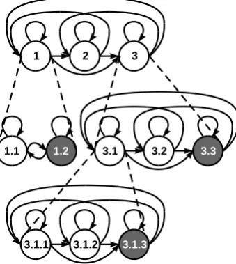
simple Gaussians, where each HMM state serves as a distinct splitting point as well as an emitting node. The resulting hierarchically tied set of HMMs somewhat resembles the well-known hierarchical hidden Markov model (HHMM) [5], nevertheless the classification tree principle considerably limits the number of states to be evaluated in every time step. Of course, boosting the evaluation speed by limiting the searched set of states introduces certain compromise to the achievable modeling performance compared to an elaborate HHMM. In the proposed structure, the most funda-mental constraint inheres in strict top-down depen-dency, i.e. lower layers have no impact on the upper layers as dictated by the classification tree principle. Consequently, sub-trees growing from individual states of a HMM in one layer do not interfere with each other. Hence, decisions made in certain position of the tree influence only nested nodes down the current tree context. Figure 1 illustrates an example of the proposed noise HMM tree structure.
1 2 3
3.1 3.2 3.3
1.1 1.2
3.1.1 3.1.2 3.1.3
Figure 1. Noise HMM tree structure
All nodes in the entire tree are emitting ones (contrasting to HHMMs where abstract nodes are usually used in all but the last layer). The root HMM consists of 3 states that compose the layer 1 of the hierarchy. Each of these states expands to a new HMM lined in layer 2. The white states of layer 2 HMMs expand further to layer 3. The dark grey nodes do not have associated sub-HMMs and inherit output distribution of the parent state. From the emission probability distribution point of view, entering such state is effectively returning parse to the parent HMM hence limiting the nesting depth. Yet, no explicit bottom-up dependence is introduced preserving the classification tree principle. This allows flexible auto-matic choice of model degree of generality based on currently observed noisy data in relation to the trained noise characteristics.
5.1. Noise Model Training
The layered structure of the proposed model is intended to catch up both general global as well as detailed local noise properties. As the hierarchy unrolls, more detailed and localized HMMs take place. Setting the model structure properly is essential for good performance, yet no exact solution to this issue is available. We decided to set the model hierarchy on the basis of unsupervised iterative hierarchical top-down segmentation employing the aforementioned BIC criterion. The segmentation algorithm is as fol-lows (symbols correspond to Eq. 7):
1) Start with (a; c) interval covering the entire trai-ning noise recording defitrai-ning the highest perspec-tive in which a boundary shall be searched for. 2) If a boundary within (a; c) is found, break the
interval into according pair and perform a new BIC search on each subinterval, i.e. (a; b) and (b;
c). If there is no boundary among (a; c) detected, divide the interval into two equal parts and run the BIC search on each of the two subintervals. Proceed recursively on all new subsections. 3) If the (a; c) interval in any iteration falls below a
preset number of segments 2ε, quit the current thread. The ε must be set reasonably to provide enough data for meaningful local statistics. The b
search within (a; c) should also be limited to (a+ε;
c-ε) interval so that the Σab and Σbc matrices have
enough training data. Utilization of diagonal matrices instead of full ones reduces the parame-ters fluctuations and allows lower ε values. The segmentation process is illustrated in Figure 2.
0 0.5 1 1.5 2 2.5 3 0
426 852 1278 1704 2130 2556
time (s)
Figure 2. Top-down iterative BIC segmentation of noise recording
Lower part of the figure shows noise spectrogram (frequency axis in logarithmic mel scale); blocks in the upper part demonstrate hierarchical structure of evaluated intervals starting with first layer on the top of the figure. Vertical black lines indicate identified
boundaries with corresponding depth of segmentation hierarchy they occurred in.
Once the hierarchical segmentation is completed, assignment of noise signal frames to HMM states can be accomplished. Our current implementation of noise model comprises 3 layers; each layer is set a prede-fined average HMM state duration (5 s, 1 s, and 0.2 s, respectively) to ensure intended "generality gradient" through the layers. Based on the predefined durations, a horizontal cut in segmentation hierarchy gives a set of BIC boundaries for the given HMM layer. Starting from the top layer, signal chunks defined by BIC bor-ders are clustered via k-means algorithm according to the intended number of HMM states. Portions of noise signal assigned to each HMM state are then concate-nated and used for GMM estimation by the split-merge EM (expectation maximization) algorithm [2] forming the state’s emission probability distri-bution. From layer 2 on, only signal portions associa-ted to corresponding state in preceding layer are used for sub-HMM construction, hence the parent state uses a superset of training samples assigned to individual states of the current layer HMM. Transition probabi-lities and priors are obtained via expected likelihood estimation (ELE) [15] from observed bigram frequen-cies. This ensures nonzero probability even for spar-sely observed transitions. Utilization of ELE plays a key role in defining the probabilities of entering the non-expanding states that are clearly never observed within the training data. ELE introduces additive smoothing to empirical probability Pˆ(y) which is computed from the observations of random variable Y
with sample space of ny possible values and (absolute) observed frequency f(y) by
Y
n k n
k y f y Y P
⋅ +
+ = = ) ( ) (
ˆ . (8)
The factor k=0.5 is dictated by the Jeffrey-Perks law [15]; n is the total number of observations. Resulting individual HMMs are ergodic ones with emitting states only.
An alternative training data/HMM state assign-ment was also considered based on Baum-Welch rees-timation and Viterbi forced alignment. After defining one layer, the resulting HMM was reestimated and new BIC segmentation was executed on all parts devolved to each state according to Viterbi alignment. Such a procedure, however, yielded worse perfor-mance than the proposed global BIC segmentation approach.
5.2. Speech Recognition Using the Noise Model
Our testing system performs isolated voice com-mands recognition by utilizing whole word left-right HMMs with usual trailing non-emitting states (see Figure 3). During the recognition, all speech HMMs are combined with the current noise HMM in current layer resulting in ergodic HMM with emitting states only. The combined model thus contains all
combi-nations of speech and noise states as well as noise-only states to account for pauses between words.
Figure 3. A word HMM (3 emmiting states, 2 non-emitting)
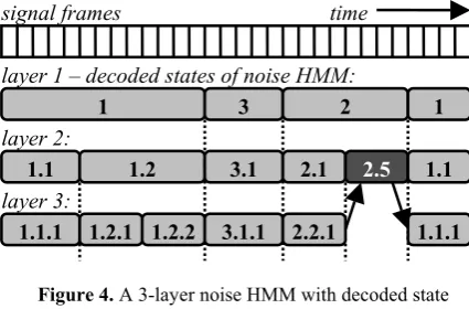
Given three layers of noise model, three Viterbi decoders must run in parallel. The first decoder uses noisy speech model where noise HMM comes from the first layer only. The Viterbi decoding selects the most probable sequence of noisy speech HMM states. From this sequence, the path through noise-only HMM is extracted (see layer 1 in Figure 4). According to parent noise HMM states in layer 1, the second Viterbi runs on noisy speech models composed of corresponding noise sub-HMMs of 2nd layer and
speech HMMs (see Figure 4 – decoded noise-only HMM states in layer 2). Analogically, the third Viterbi uses noisy speech model comprising layer 3 noise HMMs according to decoded noise HMM states in layer 2. A non-expanding state is illustrated in layer 2 (see state 2.5 in Figure 4).
Figure 4. A 3-layer noise HMM with decoded state sequence
The final outcome of noisy speech recognition, i.e. the speech HMM states sequence (and corresponding words sequence), is obtained from Viterbi decoding of noisy speech HMM associated with the last layer of noise HMM hierarchy. Speech states decoded within the upper layers are ignored as the noisy speech HMM served only for obtaining the most probable noise HMM states alignment.
Proper decoding of layers 2 and 3 requires certain modifications to the standard Viterbi algorithm [15]. Let the variable δlj(t) stores the most probable path through the trellis that leads to a node Xl
t = j, 1 ≤j≤N at time t in layer l
) | , ,
( max )
( 1 1 1 1
1 1
λ j X o o X X P
t l
t t l
t l X X l j
t
=
= − −
−
" "
"
δ (9)
where ot denotes observations and λ represents HMM parameters. The number of states N of the combined noisy speech model is given by
N N
S N N
N
N = ⋅ + (10)
1 3 2 1
1.1 1.2 3.1 2.1 2.5 1.1
1.1.1 1.2.1 1.2.2 3.1.1 2.2.1 1.1.1 layer 1 – decoded states of noise HMM:
layer 2:
layer 3:
where
∑
= = W w w N N 1 SS (11)
is the sum of the number of emitting states of all W
words (each whole word left-right HMM having NS w emitting states apart from one non-emitting state on each end) and NN is the number of states of the current
noise HMM (ergodic structure, only emitting states). Each time the noise HMM in preceding layer enters a new state, a boundary of two different noisy speech HMMs caused by unrelated noise HMMs in current layer appears (e.g. between noise states 1.2 and 3.1 in Figure 4). Yet, the “speech” portion of the noisy speech HMMs on each side of the boundary must seamlessly continue. Hence the current layer’s trellises on the left and right side of the boundary must be properly “connected”. Notice that due to variable number of states of neighboring noise HMMs the noisy speech HMMs’ number of states (and likewise the trellis vertical sizes) Nleft and Nright may vary. An iteration of δlj(t + 1) over the boundary follows the induction step of Viterbi decoding
) ( ) ( max ) 1 ( 1
1≤≤ +
=
+ ij j t
l i N i l
j t leftδ t a b o
δ , 1≤ j≤Nright (12)
where bj(ot+1) is the likelihood of observing ot+1 in state j. Factor aij represents transition probability from state i of the left trellis to the state j of the right one. Depending on the contents of the nodes i and j, 5 different formulas for obtaining aij come into question: 1) If state i within the left trellis belongs to a noisy word h(i) and state j within the right trellis belongs to the same word h(j) = h(i), then
(
) (
)+
= S f(),f( ) N g( ) )
h( i j j
aij A j π
(
f(),out)
S( ) (
f( ) N g( ))
) h( S ) h( S S )
h( j j
N W
p
i j
j
j π π
A ⋅
⋅
⋅ . (13)
2) If state i within the left trellis belongs to a noisy word h(i) and state j within the right trellis belongs to a different word h(j) ≠ h(i), then
(
)
⋅ ⋅ ⋅ = S ) h( S S )h( f(),out
j j ij N W p i a A
( ) (
f( ) N g( ))
S )
h(j j π j
π . (14)
3) If state i within the left trellis belongs to a noisy word h(i) and state j within the right trellis belongs to a noise-only state g(j) (i.e. pause between words), then
(
f(),out)
(1 S) N(
g( ))
S )
h( i p j
aij =A j ⋅ − ⋅π . (15) 4) If state i within the left trellis belongs to a
noise-only state g(i) and state j within the right trellis belongs to word h(i), then
( ) (
f( ) N g( ))
S ) h( S ) h( S j j N W p a j j
ij= ⋅ ⋅π π . (16)
5) If state i within the left trellis belongs to a noise-only state (regardless which one) and state j with-in the right trellis belongs to a noise-only state g(j), then
(
g( ))
) 1
( pS N j
aij= − ⋅π . (17)
In the preceding equations, f(i) returns a word HMM state index given noisy speech HMM state i; g(i) returns noise HMM state index given noisy speech HMM state i; h(i) returns the word index (out of W words available); AS
h(j)(u,v) is the uth row and vth
column of word h(j) HMM transition matrix (symbol “out” represents transition into trailing non-emitting state); πS
h(j)(u) is the uth element of word h(j) HMM
prior probability vector; πN denotes noise HMM prior
probability vector; pS is the probability of observing a
word; (1 - pS) is the probability of observing a pause
between words (noise-only portion of the signal). The above equations exploit the simplifying assumption that decoded states in all upper layers (from the point of view of the current layer) are all considered certain events, hence they do not explicitly figure in formulas (13) to (17). This assumption is dictated by the classification tree nature of the proposed noise model.
If the preceding layer in the current time step con-tains a non-expanding state, the noisy speech HMM for the current layer takes a special form. Since the noise-only HMM states in upper layers are now fixed, only the “speech” part of the noisy speech HMM is to be decoded. Thus the noisy speech HMM is formed by speech HMMs combined with only one noise HMM state – the one decoded in the preceding layer.
The backward Viterbi run follows standard algo-rithm with appropriate processing of the mentioned borders.
6. Experimental Results
All experiments were conducted using a 2 hours long audio recording of an operating room back-ground noise recorded during a neurosurgery at the University Hospital in Marburg, Germany. The avail-able sound data were divided into training and testing sets of equal sizes; the training set was then used for noise model construction as described earlier. HMMs in all layers were restricted to have a maximum of 5 states; smaller HMMs were occasionally inflicted by the available amount of training data assigned to the respective parent HMM state. In all experiments, feature vectors comprised of 19 MFCC coefficients computed from 32 ms frames with 10 ms advance.
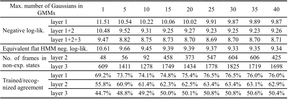
Obtained likelihoods can be found in the tables. The split-merge EM algorithm used for GMM estimation of the noise HMMs emission probabilities sets automatically the appropriate number of Gaussians. We, however, limited the maximum allowed number of Gaussians in several steps ranging from 1 to 40 to see the impact of model complexity on the overall
performance. It can be seen, that with the number of Gaussians increasing up to approx. 20, the negative log-likelihood decreases and then levels off. The tests were first conducted starting with single-layer model and then repeated with two-layer and three-layer model, respectively. Obtained likelihoods show better fit as the number of layers increases.
Table 1. Results of model fit ability to the training portion of the noise recording
Max. number of Gaussians in
GMMs 1 5 10 15 20 25 30 35 40 layer 1 11.51 10.54 10.22 10.06 10.02 9.91 9.87 9.89 9.87 layer 1+2 10.48 9.52 9.31 9.25 9.27 9.23 9.25 9.23 9.26 Negative log-lik.
layer 1+2+3 9.47 8.82 8.75 8.73 8.70 8.69 8.70 8.70 8.71 Equivalent flat HMM neg. log-lik. 10.61 9.66 9.45 9.39 9.39 9.37 9.33 9.35 9.34
layer 2 48 56 92 458 373 547 604 606 425 No. of frames in
non-exp. states layer 3 609 1411 1278 1749 1434 1778 1825 1719 1698 layer 1 69.2% 73.7% 74.1% 74.8% 75.4% 76.5% 76.5% 76.0% 76.0% layer 2 55.8% 60.9% 61.4% 62.3% 62.5% 63.4% 63.4% 63.1% 62.9%
Trained/recog-nized agreement
layer 3 44.7% 48.8% 49.2% 50.0% 50.1% 50.8% 50.8% 50.6% 50.4%
Table 2. Results of model fit ability to the testing portion of the noise recording
Max. number of Gaussians in
GMMs 1 5 10 15 20 25 30 35 40 layer 1 11.82 10.95 10.64 10.53 10.45 10.41 10.38 10.39 10.37 layer 1+2 10.84 9.98 9.83 9.78 9.78 9.77 9.78 9.76 9.77 Negative log-lik.
layer 1+2+3 9.89 9.36 9.31 9.28 9.26 9.25 9.26 9.27 9.26 Equivalent flat HMM neg. log-lik. 10.92 10.07 9.93 9.81 9.90 9.86 9.85 9.85 9.84
layer 2 43 83 86 217 330 370 334 263 285 No. of frames in
non-exp. states layer 3 660 1580 1660 1865 1868 1914 1866 1768 1834
The same task was also carried out using a traditional noise-trained flat-structured ergodic HMM with the number of states equivalent to the sum of maximal number of states in each of the three layers of the hierarchical model within one branch. Decoding using such HMM therefore involves equivalent com-putational demands. Achieved likelihoods are compar-able to something between one- and two-layered hie-rarchical model. This clearly shows, that the tested 3-layered structure provides better performance/com-putational demands ratio.
Tables 1 and 2 also show the number of frames within which the Viterbi decoder chose the non-ex-panding states in 2nd and 3rd layer (out of approx. 48k
frames total). With increasing number of Gaussians, the models are getting more specific and, subse-quently, more often the lower layers provide “over-fitted” models. This results in automatic reduction of the average depth of the used noise HMM hierarchy. It is also apparent that testing set data were more often modeled by upper layers, which corresponds with the fact that training data are logically more congruent with the given model.
The rows in Table 1 showing percentages of agree-ment between the prescribed noise HMM labels im-posed during training and actual recognized states in a given signal frames demonstrate the dependence among layers. Each lower layer depends on the upper layers, thus the amount of "hits" is ever decreasing as the depth grows. These numbers suggest that the maximum usable number of layers is not arbitrarily high and should be properly balanced according to the available amount of training data.
testing words in a random sequence divided by approx. 1 second pauses. The operating room noise was then added to the testing sound in time domain under several SNR ratios. Note that the indicated SNRs are only approximative broadly averaged va-lues, as the local power levels of the operating room noise fluctuate significantly. Table 3 summarizes ob-tained WERs (word error rates), i.e. the number of insertions I, deletions D, and substitutions S relative to the total number of words M in the recording
M I D S
WER= + + . (18)
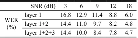
Table 3. Results of noisy speech recognition
SNR (dB) 3 6 9 12 18 layer 1 16.8 12.9 11.4 8.8 6.0 layer 1+2 14.4 11.0 9.7 8.2 4.8 WER
(%)
layer 1+2+3 14.4 10.0 8.4 7.8 4.7
The results in Table 3 support the premise of consistent performance gains with increasing number of layers used in the noise model. It is, however, also apparent that the deeper the hierarchy goes, the less pronounced the gains are. An appropriate number of layers should be therefore carefully weighted for a particular application of the proposed model based on the available amount of training data and tolerable computational demands.
7. Conclusion
The proposed nonstationary noise statistical model composed of classification tree hierarchy of HMMs presents a feasible way to increase noise robustness of ASR systems without seriously impacting the com-putational demands. Unlike traditional HHMMs, the total number of states to be evaluated in every time step is limited by the sum of maximal number of states within one branch over the given number of layers. Classification tree nature of the noise model thereby allows omitting most of the available stored HMMs and considering only the most probable ones. Experi-ments conducted on highly nonstationary operating room acoustical background noise proved better modeling ability compared to a single flat HMM with equivalent computational demands. The proposed model can be employed in any noise-robust ASR system targeted for a specific environment using a model combination approach.
Acknowledgements
Research described in the paper was financially supported by the Czech Grant Agency under grant No. 102/08/H027 and by the research program MSM 0021630513 Advanced Electronic Communication Systems and Technologies (ELCOM). Authors wish to thank Prof. Dr. med. Christopher Nimsky and Dr. med. Christoph Kappus for allowing the sound
recording in the operating room at the University Hospital in Marburg and Prof. Dr. Detlef Richter for valuable support.
References
[1] A. Acero, L. Deng, T. Kristjansson, J. Zhang. HMM Adaptation Using Vector Taylor Series for Noisy Speech Recognition. In Proceedings of ICSLP 2000, Beijing, 2000, 869 – 872.
[2] K. Blekas, I. E. Lagaris. Split-merge incremental learning (SMILE) of mixture models. In Proceedings of ICANN 2007, Porto, 2007, 291 – 300.
[3] P. Divenyi. Speech Separation by Humans and Ma-chines. Kluwer Academic Publishers, 2005.
[4] K. Driaunys, V. Rudžionis, P. Žvinys. Implemen-tation of Hierarchical Phoneme Classification Ap-proach on LTDIGITS Corpora. Information Techno-logy and Control, 2009, Vol. 38, No. 4, 303 - 310.
[5] S. Fine, Y. Singer, N. Tishby. The hierarchical hid-den Markov model: analysis and applications.
Machine Learning, 1998, Vol. 32, 41–62.
[6] M.J.F. Gales, S.J. Young. Robust continuous speech recognition using parallel model combination. IEEE Transactions on Speech and Audio Processing, 1996,
Vol. 4, No. 5, 352–359.
[7] M. Graciarena, H. Franco. Unsupervised noise mo-del estimation for momo-del-based robust speech recognition. In Proceedings of ASRU IEEE Workshop on Automatic Speech Recognition and Understanding, 2003, 351-356.
[8] H. Hermansky. Perceptual linear prediction (PLP) analysis of speech. Journal of the Acoustical Society of America, 1990, Vol. 87, No. 4, 1738–1752.
[9] H. Hermansky, N. Morgan. RASTA processing of speech. IEEE Trans. on Speech and Audio Processing, 1994, Vol. 2, No. 4, 578–589.
[10] D. Jurafsky, J.H. Martin. Speech and Language pro-cessing: An Introduction to Natural Language Proces-sing, Computational Linguistics, and Speech Recogni-tion. Prentice Hall, 2009.
[11] H.K. Kim, R.Rose. Cepstrum-domain model combi-nation based on decomposition of speech and noise for noisy speech recognition. In Proceedings of ICASSP-2002, 2002, 209-212.
[12] D. Kim, D. Yook. Fast Channel Adaptation for Con-tinuous Density HMMs Using Maximum Likelihood Spectral Transform. IET Electronics Letters, 2004,
Vol. 40, No. 10, 632 – 634.
[13] T. Kosaka, H. Yamamoto, M, Yatnada, Y. Komori. Instantaneous environment adaptation techniques based on fast PMC and MAP-CMS methods. In Proceedings of ICASSP, Atlanta, 1998, 789–792.
[14] C.J. Leggetter, P.C. Woodland. Maximum Like-lihood Linear Regression for Speaker Adaptation of Continuous Density Hidden Markov Models.
Computer Speech & Language, 1995, Vol. 9, No. 2, 171 – 185.
[16] G. Matz, F. Hlawatsch, A. Raidl. Signal-adaptive ro-bust time-varying Wiener filters: best subspace selection and statistical analysis. In Proceedings of ICASSP-2001, Salt Lake City, 2001, 3945–3948.
[17] S. Rennie, T. Kristjansson, P. Olsen, R. Gopinath. Dynamic Noise Adaptation. In Proceedings of ICASSP-2006, Vol. 1, 2006.
[18] R. Rose. Environmental robustness in automatic speech recognition. In Proceedings of Robust 2004, Norwich, 2004, 1-7.
[19] S. Shaobing, P. Gopalakrishnan. Speaker, environ-ment and channel change detection and clustering via the Bayesian information criterion. In Proceedings of DARPA Broadcast News Transcription and Understanding Workshop, Virginia, 1998, 127-132.
[20] R.C. Van Dalen, M.J.F. Gales. Covariance Model-ling for Noise-Robust Speech Recognition. In Proceedings of INTERSPEECH 2008, Brisbane, 2008.
[21] K. West, S. Cox. Features and classifiers for the automatic classification of musical audio signals. In Proceedings of ISMIR '04, Barcelona, 2004.
[22] H. Xu, Z. Tan, P. Dalsgaard, B. Lindberg. Robust Speech Recognition Based on Noise and SNR Classi-fication – A Multiple-Model Framework. In Procee-dings of INTERSPEECH-2005, Lisbon, 2005, 977 – 980.
[23] U. Yapanel, J.H.L. Hansen, R. Sarikaya, B. Pellom. Robust digit recognition in noise: an evaluation using the Aurora corpus. In Proceedings of
EUROSPEECH-2001, Aalborg, 2001, 209–212.
[24] K. Yuo, H. Wang. Robust Features for Noisy Speech Recognition Based on Temporal Trajectory Filtering of Short-Time Autocorrelation Sequences. Speech Communication, 1999, Vol. 28, No. 1, 13 – 24.
[25] P. Zelinka, M. Sigmund. Towards Reliable Speech Recognition in Operating Room Noise Environment.
In Proceedings of Radioelektronika 2010, Brno, 2010, 31 – 34.