promoting access to White Rose research papers
Universities of Leeds, Sheffield and York
http://eprints.whiterose.ac.uk/
This is an author produced version of a paper published in
Transportation
Research Part B: Methodological.
White Rose Research Online URL for this paper:
http://eprints.whiterose.ac.uk/43556/
Paper:
Carey, M (2012)
Dynamic traffic assignment approximating the kinematic wave
model: system optimum, marginal costs, externalities and tolls.
Transportation
Dynamic traffic assignment approximating the kinematic wave model: system optimum, marginal costs, externalities and tolls
Malachy Carey. Institute for Transport Studies, University of Leeds, Leeds LS2 9JT. Tel: +44 28 90 203 659, Email: [email protected]
Abstract
System marginal costs, externalities and optimal congestion tolls for traffic networks are generally derived from system optimizing (SO) traffic assignment models and when these are treated as varying over time they are all referred to as dynamic. In dynamic SO network models the link flows and travel times or costs are generally modelled using so-called „whole link‟ models. Here we instead develop an SO model that more closely reflects traffic flow theory and derive the marginal costs and externalities from that. The most widely accepted traffic flow model appears to be the LWR (Lighthill, Whitham and Richards) model and a tractable discrete implementation or approximation to that is provided by the cell transmission model (CTM) or a finite difference approximation (FDA). These handles spillbacks, traffic controls and moving queues in a way that is consistent with the LWR model (hence with the kinematic wave model and fluid flow model). An SO formulation using the CTM is already available, assuming a single destination and a trapezoidal flow-density function. We extend the formulation to allow more general nonlinear flow density functions and derive and interpret system marginal costs and externalities. We show that if tolls computed from the DSO solution are imposed on users then the DSO solution would also satisfy the criteria for a dynamic user equilibrium (DUE). We introduce constraints on the link outflow proportions at merges and inflow proportions at diverges. We also extend the model to elastic demands and establish links with previous dynamic traffic assignment (DTA) models.
Keywords: cell transmission model; system optimum; dynamic traffic assignment; marginal costs;
externalities; optimal tolls
1. Introduction
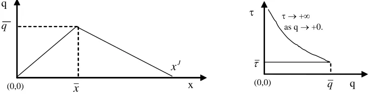
This paper is concerned with deriving system marginal costs, externalities and hence system optimizing congestion tolls for road networks when traffic flows and travel times are varying over time. In view of that it adopts a dynamic system optimizing (DSO) formulation. We present and analyse a DSO model for dynamic traffic assignment (DTA) in which the traffic flows are modelled by approximation to the widely accepted traffic flow model originated by Lighthill and Whitham (1955), Richards (1956), referred to as the LWR model. Since the latter is a differential equation model, continuous in time and space, it is not analytically or computationally tractable for general traffic network modelling and it is more convenient to approximate it by a finite difference approximation, as in Daganzo (1994, 1995a, 1995b). Daganzo (1994, 1995a) developed the cell transmission model (CTM) that approximates the LWR model when the flow-density function is assumed to be triangular or trapezoidal, as in Fig. 1. Daganzo (1995b) extended the analysis to allow general nonlinear flow-density functions as in Fig. 2 and refers to this model as a finite difference approximation (FDA) to the LWR model. For brevity we will often refer to both the CTM and FDA model as the CTM. For each of these models he showed that as the discretisation of time and space is refined to the continuous limit the model converges to a correct solution of the LWR model.
In the above papers and in various later papers the CTM in a network context is usually presented as a simulation model in which traffic at junctions and intersections merges and diverges in fixed proportions at each point in time and route choice is fixed. Later the CTM was used as the network loading
prespecified. To solve the user equilibrium formulation the spatial route allocations are iteratively adjusted until an equilibrium is achieved.
Ziliaskopoulos (2000) reformulated a relaxed form of the CTM as a set of linear constraints and hence developed a linear programming model for the single-destination system optimum DTA problem for a network. The model was further analysed and applied by Waller (2000), Li et al. (2003), Alecsandru (2006), Ukkusuri and Waller (2008), Zeng (2009 and Lin and Liu (2010). The present paper introduces a similar system optimizing formulation, though it instead assumes that the flow-density function for each link may have a general nonlinear form rather than the triangular or trapezoidal form usually assumed in the CTM. The latter forms can be thought of as special cases of a general nonlinear form. This yields a nonlinear convex DSO model rather than a linear programme.
Though this paper is concerned with marginal costs, externalities and optimal congestion tolls or prices for road traffic it does not further pursue the various aspects of congestion pricing. For a comprehensive discussion of the mathematical and economic theory of road pricing see Yang and Huang (2005). Also, the focus in the paper deterministic rather than stochastic: some recent stochastic extensions and
applications of the CTM can be found in Karoonsoontawong and Waller (2005), Alecsandru (2006), Boel and Mihaylova (2006), Szeto (2008) and Sumalee et al. (2010).
For various reasons we assume a general nonlinear form of flow-density function rather than the usual triangular or trapezoidal form. First, it can include the piecewise linear forms as special cases. Second, in some cases one may wish to avoid some properties of the triangular or trapezoidal form. For example, a triangular flow-density function implies that travel time as a function of flow is initially a horizontal line until it switches to backward-sloping (as in Fig. 1(b)), and a trapezoidal flow-density function has a similar implication except that the travel time function has a vertical piece before sloping backwards. Neither form allows an upward sloping travel time function, which is widely used in static traffic
assignment. A further and more immediate reason for assuming a nonlinear flow-density function in this paper is that it can be assumed differentiable whereas piecewise linear forms are not. Differentiability is very convenient for the derivation and analysis of marginal costs in this paper. However, for readers who prefer a triangular or trapezoidal flow-density function, or a more general piecewise-linear flow-density function, it is worth noting that a nonlinear differentiable curve can be chosen to fit as closely as we wish to any piecewise linear curve. To obtain a smooth differentiable curve we need only assume an arbitrarily small rounding or smoothing at the break-points of the piecewise linear curve. This rounding can be assumed so small that it does not affect numerical results – is less than the working tolerance in computations.
q
x
xq
(0,0)
J
x
+ as q +0.
q q
(0,0)
[image:3.612.111.490.535.632.2]
Fig. 2. A nonlinear flow-density or flow-occupancy function.
A system optimising formulation can lead to the phenomenon of “holding back” of flows on some links, which has been identified by a number of authors as a common feature in models that seek to optimize traffic flows on a network over time. By holding back some of the traffic that would otherwise enter a link it may be possible to keep the traffic density from moving onto the downward-sloping (congested) part of the flow density function. Moving onto that portion of the curve would reduce the traffic outflow and eventually cause a reduction in inflow and throughput and hence increase overall system travel times or costs. Holding back of traffic could be used to reduce or prevent that and hence can be interpreted as a desirable form of traffic flow control (as in Carey (1987) and Ziliaskopoulos (2000)). Such flow controls could potentially be implemented by variable speed controls, ramp metering or other methods associated with future intelligent traffic and transport systems.
Section 2 outlines the Daganzo (1995a) finite difference approximation to the LWR model and re-writes the max function from this as inequalities. This allows flow controls of the type mentioned in the previous paragraph. Section 3 extends this formulation from a single link to a network of such links and formulates the traffic DSO assignment problem as a convex nonlinear programme. The merge and diverge proportions at junctions are determined endogenously within the programme so as to minimize travel costs or maximise traveller net benefits. Section 4 derives, analyses and interprets optimality conditions, marginal costs, externalities and optimal tolls. Section 5 introduces constraints on merge and diverge proportions at junctions (nodes) to more realistically reflect actual constraints on these. Section 6 discusses extending to cost-elastic travel demand functions and Section 7 concludes. Appendix A considers relationships between the CTM and the Merchant-Nemhauser model and Appendix B considers other forms of cost-elastic travel demand functions for Section 6.
2. A finite difference approximation to the LWR model
The LWR traffic flow model (Lighthill and Whitam (1955) and Richards (1956) assumes that the flow at each point in space and time (z,t) depends only on the density at that point, and not at any later or earlier points, hence can be stated as a flow-density equation q(z,t)Q(k(z,t),z,t). Here, as is commonly done, we assume that the link is homogeneous over space and time: if capacity changes along a link it can be sub-divided into homogeneous links. This reduces the flow-density function to
)) , ( ( ) ,
(z t Qk z t
q (1)
In the LWR model this is combined with a conservation or continuity equation
t t z k z t z
q
( , )/ ( , )/ (2)
To approximate (1)-(2) by a difference equation Daganzo (1995b) discretised (1)-(2) as follows. Divide the time span into time intervals t = 1, …, T, each of length t, and divide the link into j = 1, …, J, segments or cells such that the free-flow travel time for each cell is one time interval. This satisfies the Courant-Friedrichs-Lewy (CFL) condition (Courant et al. (1967)) that the cell lengths travelled per time
q q
x
J
x
x
step should not exceed one, which is a necessary condition for the convergence of a finite difference approximation to solve a partial differential equation as the step sizes go to zero. Daganzo shows that the scheme converges without explicitly referring to the CFL condition.
We can assume that the given link is homogeneous, so that all cells will be of the same length d. Let kjt
denote the cell density, which can be assumed constant along the cell length or can be taken as the mean density in the cell. The flow-density function for a cell can then be written as qjt Qj(kjt), but it is
convenient here to work in terms flow-occupancy xjt kjtd rather than flow-density kjt. Substituting
d x
kjt jt/ in the flow-density function gives the flow-occupancy function denoted gj(xjt). From the
latter, construct two functions gj(xjt) and gj(xjt): gj(xjt) is obtained by taking the upward sloping
part of gj(xjt) and extending it to the right via a horizontal straight line from its peak, and gj(xjt) is
obtained by taking the downward sloping part of gj(xjt) and extending it back to the vertical axis via a
horizontal straight line from its peak. Then, as in Daganzo (1995b), for consistency with the continuous LWR model, the number of vehicles exiting from cell j into the next downstream cell j+1 in time interval t should satisfy
jt
v = min{gj(xjt), gj1(xj1,t)} (3) = min{(sending capacity of cell j in time interval t),
(receiving capacity of the next downstream cell j+1 in time interval t)}.
Except for the final cell on a link, the outflow vjt from cell j in any time interval equals the inflow uj1,t
to next downstream cell j+1 in the same interval, thus
t j jt u
v 1, (4)
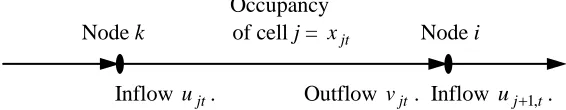
as illustrated in Fig. 3. The number of vehicles in cell j in time interval t+1 is the number present in time interval t plus the inflow minus the outflow in interval t, thus,
jt jt jt t
j x u v
x ,1 (5)
Equations (3)-(5) comprise a finite difference approximation to the LWR model (1)-(2). Equation (3) can
be rewritten as vjt gj(xjt) and vjt gj1(xj1,t) if we assume for the moment that the outflow vjt is held at the maximum consistent with these inequalities, so that one or other of these inequalities is a strict equality. In that case (3)-(4) can be rewritten as
) ( jt j
jt g x
v and uj1,t gj(xj1,t) (6.1)
if the flow vjt uj1,t is at the maximum consistent with (6.1). (6.2)
The finite difference approximation to the LWR model now consists of (4)-(6.2). The advantage of the inequalities in (6.1), for the purposes of a mathematical programming model below, is that they represent convex sets, since gj(xjt) and gj(xj1,t) can be assumed to be concave functions. In contrast, (3) is a
If the flow vjt uj1,t is less than the maximum given by (6.1) then the outflow from cell j to j+1 will is
less than the flow rate given by the CTM equation (3). However, this shortfall may be interpreted as a traffic control system “holding back” the “natural” flow rate, as already mentioned in the Introduction.
Occupancy
Node k of cell j = xjt Node i
[image:6.612.89.372.132.187.2]Inflow ujt. Outflow vjt. Inflow uj1,t.
Fig. 3. Inflow, outflow and occupancy (ujt, vjt and xjt) for cell j.
3. A system optimising DTA model based on a finite difference approximation to the LWR model
Consider a network consisting of a set of nodes NO connected by a set of directed links AO, with individual nodes and links denoted i NO and j AO respectively. Let each of the original links in the network be divided into cells, introduce an artificial node between each pair of neighbouring cells and treat each cell as a link between these neighbouring nodes. Denote this expanded set of nodes as N and expanded set of links as A, thus NON and AOA. Let B(i) denote the set of links immediately before node i (pointing into node i) and A(i) denote the set of links immediately after node i (pointing out of node i).
Extending the cell conservation equation (5) to a network. To extend (5) to the network, simply rewrite it
for all cells j A in the network, thus
jt jt jt t
j x u v
x ,1 jA. (7)
Extending the node conservation equation (4) to a network. To ensure conservation at all nodes i N of
the network, let the sum of the inflows to each node equal the sum of the outflows from the node, thus
jA(i)ujt Dit jB(i)vjt i N (8)
where Dit is the exogenous travel demand from node i to the destination. We can assume an artificial link or cell exiting from the destination node. For the new nodes along the original links (nodes i N, i NO),
it
D = 0 and (8) reduces to (4), i.e. vjt uj't where j' is the (single) cell immediately after cell j.
Extending the exit flow equations (6.1)-(6.2) to a network.
Applying (6.1) and (6.2) to all cells on all links we have the following. For each cell j the outflow vjt should not exceed the sending capacity gj(xjt) of the cell, thus,
) ( jt j
jt g x
v . j A (9.1)
and for each cell j the inflow ujt should not exceed the inflow capacity or receiving capacity gj(xjt)
of
the cell, thus,
) ( jt j
jt g x
and
either (9.1) or (9.2) is a strict equality j A. (9.3)
Condition (9.3) is needed to be consistent with (6.2) and hence (3). However, we wish to construct a mathematical programming model for system optimizing and an either-or constraint such as (9.3) converts a convex programme to a combinatorial problem or 0-1 integer programme, which is nonconvex. Such a programme is potentially very time consuming to solve because of the very large number of cells in the network. Fortunately, in the mathematical programme that we construct later below, condition (9.3) is frequently satisfied in a solution of the mathematical programme without having to be imposed as an explicit constraint. Furthermore, any deviation from satisfying (9.3) may be interpreted as a system optimising flow control, as noted in the Introduction.
A system optimising DTA model
We can now set up a system optimising dynamic traffic assignment model, consisting of minimising the network travel costs for all users, subject to the constraints (7)-(9.2). Let the length of each time interval be 1. Then the total time spent by users xjt in cell j in time interval t is 1xjt, the total time spent by all
users on the network is
Tt1 jAxjt and the total cost of this user time is
T
t j Acjtxjt
C 1 (10)
where cjt is the users‟ cost per unit of time spent in cell j in time interval t. To obtain system optimising
flows on the network, minimise (10) subject to (7)-(9.2) and nonnegativity of all the variables. This is set out more formally as follows.
S: Minimise (10)
subject to, for all time intervals t = 1, …, T,
(jt 0) vjt gj(xjt) j A (11.1)
(jt 0) ujt gj(xjt) j A (11.2)
(jt) xj,t1 xjt ujt vjt j A (11.3)
(it) jA(i)ujt Dit jB(i)vjt i N (11.4)
xjt 0, ujt 0, vjt 0 jA. (11.5)
The variable in brackets before each equation (i.e., jt 0, jt 0, jt and jt) is a dual variable or
In model S it is implicitly assumed that at a merge node the flows on the links pointing into the junction (node) can enter it in any proportions, subject only to flow conservation. Similarly, at a diverge node it is assumed that the flows on the links pointing out of the junction can exit from it in any proportions. However, the layout of the junction and/ or the traffic control system may impose additional restrictions on these proportions. This is ignored here but is reintroduced in Section 5. Until then it can be assumed that the layout and controls can be adjusted to accommodate whatever solution is given by Programme S.
It is interesting to consider what happens if the equations (11.2) are dropped from the above model S. Equations (11.2) are redundant if all links in the solution of S are uncongested, that is, if the cell
occupancies xjt are never in the downward sloping part of the exit-flow functions gj(xjt). Without
(11.2), the above model becomes formally the same as the DTA model of Merchant and Nemhauser (1978a, 1978b) except that, in the latter, the equations (11.1) are written as strict equalities whereas here they relaxed to inequalities. The MN model with (11.1) as inequalities was introduced by Carey (1987), where it was noted that it converts the nonconvex optimisation model of MN to a convex model. The latter is formally the same as the above model, except that the MN model has usually been applied to networks with each link treated as a whole link. However, the MN model can equally well be applied after first discretising the whole links into cells and discretising time as in the above model S. Further relationships between the CTM, FDA and LWR models on the one hand and the MN model on the other are discussed in Appendix A and in Carey and McCartney (2004).
Solving programme S.
The above convex nonlinear programme S is linear except for the concave functions in (11.1) and (11.2) hence can be solved easily in various ways. It can be solved by using linear programming if we first piecewise linearise the concave functions (11.1) and (11.2). Many commercial LP (or mathematical programming) packages include a facility for automatically performing such piecewise linearization. Alternatively, the programme S can be solved using available commercial packages for solving convex programming problems with nonlinear constraint (e.g., Minos, Conopt, or other solvers available with GAMS). Or special purpose solution algorithms can be devised to take advantage of the special structure of the model. As already noted, the programme S is similar to the form of DTA model formulated in Merchant and Nemhauser (1978), except for the additional constraints (11.2). Various algorithms were devised to take advantage of the structure of the latter model and these could be extended to the present model. The model S also has another special feature which would speed up its solution: most of the links j in S were formed by discretising the original links in the network, hence are have only a single link (cells) pointing in and out of them. That simplifies the structure and greatly increases the sparsity of the matrix of constraint coefficients, which may make standard mathematical programming algorithms competitive with special purpose algorithms.
4. Properties of the model: system marginal costs, externalities and optimal tolls
To investigate the properties of solutions of Programme S we use the Kuhn-Tucker (K-T) optimality conditions which can be set out as below. These conditions are necessary and sufficient to characterise an optimal solution of S since the objective function and constraint set of S are convex.
The K-T conditions for Programme S consist of the following, for t = 1, …, T:
Equations (11.1)-(11.5) (12.0)
(ujt 0) jt kt jt, j A(k), k N (12.1)
(vjt 0) jt it jt, j B(i), i N (12.2)
(xjt 0) jtgj'(xjt)jtgj'(xjt)cjt (jt j,t1), j A (12.3)
Complementarity for the pairs of inequalities in (12.1)-(12.3).
Complementarity or „complementary slackness‟ means that, in a solution of the K-T conditions, if either one of a pair of inequalities is a strict inequality then the other one must be a strict equality.
To interpret the above optimality conditions we first consider the system marginal costs (s.m.c‟s). In a constrained optimisation programme such as S, the Lagrange multiplier or dual variable associated with any constraint is the amount by which the optimal value of the objective function will change per unit change in the value of a constant term in the constraint, such as the Dit term in (11.4), while holding all other parameters fixed. This is also referred to as the system marginal cost, hence it is the s.m.c. of increasing Dit. Since a unit increase in Dit will move through the network, governed by (10)-(11.5), until it exits at the destination, it can be described as the s.m.c. of travelling from node i in time interval t to the destination.
In a similar way the dual variables in (12.1)-(12.2), i.e. jt, kt, it, jt and jt, can be interpreted as follows. For time interval t:
jt
is the s.m.c. of adding an extra unit of traffic to cell j in (11.3), i.e. the s.m.c. of travelling from cell j to the destination.
kt
and it are the s.m.c‟s per extra unit of traffic travelling to the destination from node k (at the
entrance of cell j) and node i (at the exit of cell j) respectively.
jt
and jt are s.m.c‟s incurred by the capacity restrictions (11.1) and (11.2) on entering and exiting cell j.
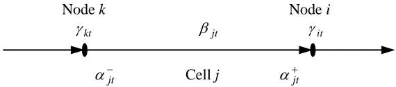
The K-T equations (12.1) and (12.2) (i.e. kt jt jt and jt it jt) contain similar variables, hence to illustrate the difference between them, Fig. 4 places these dual variables alongside the
components of the network with which they are associated (jt beside cell j, jt and jt beside the
entrance and exit respectively of cell j, and kt and it beside the nodes at the entrance and exit
respectively of cell j). Equation (12.1) states that the first variable in Fig. 4 (i.e. kt, starting from the left) is the sum of the next two variables. Equation (12.2) states that the third variable in Fig. 4 (i.e. jt) is
the sum of the next two variables.
Node k Node i kt jt it
[image:9.612.88.373.618.681.2]jt Cell j jt
Proposition 1. Let Pit denote the set of time-space paths from node i to the destination setting out in time interval t. Then in an optimal solution of programme S
(a) the s.m.c. of traversing the utilised time-space paths Pit is given by the value the dual variable it in the optimal solution of S, hence
(b) is the same for all utilised the time-space paths in Pit and
(c) is less than or equal to the s.m.c. of traversing any unutilised time-space path in Pit.
Proof. We can show this in the same way as is done for static traffic assignment but since the expressions
and summations involved are much more cumbersome than for the static traffic assignment model we do not write them out here in full.
(a) As noted above, this follows from the usual interpretation of dual variables.
(b) Along any utilised time-space path Pit the cell and link inflows ujt, outflows vjt and occupancies
jt
x must be positive which, by complementarity in the K-T conditions, means that the corresponding
equations (12.1)-(12.3) will be strict equalities. In that case we can write these equations for each cell along the time-space path and, by sequential substitution, express the it at the start of the path as a sum of cell s.m.c. terms along the path. But since the sum for each utilised path is it and it is independent of path (has no path subscript), the sum is the same for all paths.
(c) Along any time-space path Pit that is not utilised, some of the cell and link inflows ujt, outflows vjt
or occupancies xjt may be positive (as in (a)) but at least one of them must be zero, otherwise the path
would be utilised. Again, by complementarity in the K-T conditions, this means that at least one of the corresponding equations (12.1)-(12.3) will be a strict inequality. In that case, when we perform sequential substitution from (12.1)-(12.3) along the time-space path we obtain it the sum of the s.m.c. terms
along the time-space path.
4.1. System marginal costs, externalities and optimal tolls
For congested road traffic, an additional or marginal traveller tends to cause an increase in travel times or costs for other users and this increase in costs is referred to as the congestion externality caused by the additional user. It is normally assumed that, when deciding whether or when to travel, each road user takes account only of the travel time or cost that they experience and does not take account of any congestion externality. The total cost caused by an additional (marginal) user of a road path, link or cell is referred to as the system marginal cost (s.m.c.) and is (the cost experienced by a marginal/ additional user) plus (the congestion externality caused by the marginal/ additional user). If a toll just equal to the externality is imposed on each user then the total cost experienced by each user (own cost + toll) becomes equal to the s.m.c. so that the user is induced to take account of the full s.m.c. when making travel
decisions. In other words, the user is induced to "internalise" the externality and the resulting user equilibrium will also be a system optimum.
Computation of path travel times itp and link travel times. Let itp denote the travel time experienced by
a user travelling from node i at time t to the destination via spatial path pPit. In CTM based models, and other exit flow models, this is computed by a cumulative flow method, comparing the cumulative inflow and outflow from a path, e.g. if the n‟th user enters a spatial path at time t1 and exits from it at time t2 then the path travel time is t2 – t1. For further details of this method of computing travel times see for Cayford, Lin and Daganzo (1997), Tong and Wong (2000) and Lo and Szeto (2002)). Link or cell travel times are computed in the same way, the only difference being in the location of the points at which the cumulative flows are computed.
Definition of DUE:
Let Pit denote the set of time-space paths starting from node i in time interval t and travelling to the destination. Then a flow pattern is a DUE if and only if, for each it
(a) the travel time/ cost experienced by users is the same for all utilised time-space paths in Pit and (b) is less than or equal to the travel times/ costs for unutilised time-space paths in Pit.
Note that the following discussion and propositions do not provide a general DUE model based on the CTM in the absence of optimal tolls. It instead allows us only to take a DSO model based on the CTM (i.e. S) and from it derive tolls that, if imposed on users, will ensure that the DSO solution is also a DUE. A DUE methodology based on the CTM is developed in Ukkusuri (2002) and Ukkusuri and Waller (2008). In that approach the objective function is not initial fully specified but instead certain cost or penalty parameters have to be iteratively adjusted to force the solution ever closer to a DUE solution. It seems not possible to-date to develop an analytic DUE model analogous to the above CTM based SO model. As a result it has not been possible to take a DUE model based on the CTM, insert tolls in the cost function and obtain an analytic solution to examine how the tolls affect the solution.
Since the link and path travel times can be computed only after solving the Programme S, we have to take a quite different approach to obtaining optimal tolls than is followed in static assignment models.
Proposition 2.
Take a solution of Programme S and in the solution divide the set of spatial paths Pit from each it into
two sets, utilized Pitu and unutilized Pitun. Define tolls
p it it p it
toll for paths pPitu
p it it p it
toll (e.g. tollitp it itp + a constant) for paths pPitun
where the itp are as defined above and the it‟s are the values of the dual variables (s.m.c‟s) from the solution of Programme S or its dual.
If these tolls are imposed on users of the network then they will choose a user equilibrium flow pattern that is identical to the solution of Programme S, i.e. the DUE will also be a DSO.
Proof. The travel times experienced by users on paths pPit are itp hence if tolls
p it it p it
toll are
imposed on paths in Pitu then the cost experienced by users of these paths is itp (it itp)it and if
tolls tollitp it itp are imposed on paths in Pitun then the cost experienced by users of those paths is
it p it p
it toll
Proposition 3. The path s.m.c‟s, travel times and tolls in Proposition 2 can be decomposed into the sum of s.m.c‟s, travel times and tolls respectively on the time-space links along each time-space path. For example, the s.m.c‟s for traversing successive links along a time space path are it i't', i't'i"t", etc. , i.e. the differences between the it‟s for successive nodes. Similarly for link travel times and tolls.
Proof. The s.m.c‟s for traversing successive links along a time space path are it i't', i't'i"t", etc. ,
i.e. the differences between the it‟s for successive nodes.
From this definition of link s.m.c‟s it follows immediately that their sum along a time-space path is the s.m.c. it for the initial node of the path minus the s.m.c. for the final node. The latter is zero hence the sum is simply the path s.m.c. it. Replacing the ‟s with ‟s in the preceding sentences gives the same result for link travel times i't'i"t" and their sums on time-space paths. The tolls are the differences between the s.m.c‟s and the travel times hence the same result holds for those, i.e. the sum of link tolls
along a time-space path equals the path toll.
It is worth noting a discretisation issue which arises in summing s.m.c‟s, externalties or tolls along a time-space path. The s.m.c. of travelling to the destination from node i at the entrance of link j in time interval t is it and from node i at the exit of link j at time e(jt) is i,e(jt). Hence the s.m.c. of a vehicle using link
j, entering it in time interval t, is (it – i,e(jt)). Note that traversing the link may take a non-integer
number of time intervals, hence the exit time e(jt) may not have an integer value, hence may not correspond to exactly the beginning or end of one of the time intervals t in the model. Because of that, the dual variable i,e(jt), defined above, may not be associated with the equation (11.4) for a specific
(integer) time interval t , hence would not be immediately available in the solution of programme S. However, in that case we can compute i,e(jt) by interpolating between the values of it' for adjacent
integer times, that is, compute i,e(jt) by interpolating between it' and i,t'1 where t < e(jt) < t +1, for
example by using linear interpolation.
We have not shown that the path tolls in Proposition 2 or link tolls in Proposition 3 are always positive.
However, in Proposition 4 below we show that if a constant (say cR) is added to each of the tolls in Proposition 2, the resulting new tolls still satisfy Proposition 2, hence retain a DSO that is also a DUE.
Thus, if any of the path tolls from Proposition 2 are negative, a cR can be added to each path toll to
ensure that all path tolls become zero or positive. For example, set cR equal to the most negative of the
path tolls. Also, this additional flat toll cR brings in a revenue cRD where D
Tt1Dt hence cR can be adjusted to bring in any desired level of additional revenue while retaining a DSO that is also a DUE.Proposition 4. From Programme S construct a new programme SR by imposing an additional cost cR
on each unit of flow exiting at the destination, i.e. add cR
Tt1ujDt to the objective function to beminimized, where jD is an artificial link pointing out of the destination node. This:
(a) increases the total system cost by a fixed amount cRD where D
Tt1Dt ,(b) makes no change in the optimal solution set of S, i.e. {uitR,vitR,xitR} = {uit,vit,xit},
(c) increases the s.m.c. it at each time-space node by cR, so that the new dual solution is it R R
it c
(d) increases each of the optimal path tolls by cR to tollitpRtollitp cR.
Remarks. The above results indicate that the optimal path tolls are not unique but can be scaled up or
down by adding cR to each path toll, without affecting the DSO/ DUE solution. Since (a)-(d) indicate
exactly how the optimal solution of S and its dual are affected by imposing an extra cost cR on each unit
of inflow, there is no need to need to actually solve the new programme SR or its dual to find the new solution. They are already given by (a)-(d).
Note that the tolls it itp do not appear in the objective function of programme S; only the additional
tolls cR appear there. Also, note that Programme S is convex programme hence either has a global optimum and a single optimal solution or a convex set of solutions (all of which yield the same optimal value).
Proof. (a)-(b). All of the fixed travel demand D
iN Tt1Di in S has to eventually exit into theartificial link jD hence
Tt1ujDt = D hence
T t j t R
D
u
c 1 = cRD. But the latter is a constant hence
Tt j t RD
u
c 1 is a constant and adding a constant to the objective function of a convex programme S has
no effect on an optimal solution of S, except that the optimal value of the objective function is increased
by a fixed amount cRD.
(c). Consider the dual of Programme S. Since S is a convex programme there is no duality gap, that is, the
optimal value of S and its dual are equal. The objective function of the dual is
iN Tt1Ditit . We haveseen that adding cR
Tt1ujDt to the objective function of S increases its optimal value by a constantD
cR = cR
iN Tt1Dit hence increases the optimal value of the dual programme by the same amount,thus
iN Tt1DititR = cR
iN Tt1Dit +
iN tT1Ditit . But itR it cR solves this equation hence is an optimal solution of the dual.(d). From Proposition 2 the optimal path toll is it itp (i.e. the path s.m.c. it minus the path travel
time). itP is computed from the solution of S and since the latter is unchanged by introducing cR (see
(b)) the path travel times are also unchanged, i.e. itpR itp. Also, from (c), the new s.m.c‟s are
R it R
it c
. Hence the new optimal tolls are tollitpR itRitpR= (it cR)itp= tollitp cR.
4.2. Relationships between components of system marginal costs for paths
S.m.c‟s are used above to obtain optimal congestion tolls, but there are also other possible uses for the s.m.c‟s obtained from the solution of programme S. For example, in time interval t the s.m.c. of travelling to the destination from nodes k or i are kt and it respectively hence the s.m.c. of letting a vehicle (a marginal unit of traffic) enter at node k instead of node i in time interval t is (kt it). Similarly, the s.m.c. of letting a vehicle enter at node i in time interval t instead of in time interval t is (i,t it).
In 4.1 we considered the path s.m.c. that is incurred by an additional unit of traffic entering at node i, which is given by it the dual variable associated with the conservation equation (11.4) for node i. In the discussion below it is instead convenient to consider a path as starting from a link or cell j pointing into node i. The s.m.c. for this path is given by the dual variable jt associated with the conservation
equation (11.3). We can interpret jt and it as follows, for time interval t:
jt
= is the s.m.c. of an additional unit of traffic entering cell j and traveling from there to the destination.
it
= is the s.m.c. of an additional unit of traffic entering at node i (at the exit of cell j) and traveling from there to the destination.
The discussion in Section 4.1 was concerned mainly with the paths and the original links rather than the cells into which these are divided. However, the discussion below refers mainly to the cells.
For traffic entering cell j in time interval t1, the path s.m.c. is j,t1 and by rearranging the K-T
condition (12.3) we can express this as
) ( ' ) ( ' 1
,t jt jt jt j jt jt j jt
j c g x g x
(12.3‟)
It is unusual for both jt and jt to be nonzero for a cell j. A nonzero jt means that (11.1) is binding,
i.e., the outflows vjt from cell j are on the nondecreasing (or upward sloping) part gj'(xjt) of the
flow-density function. A nonzero jt means that (11.2) is binding, i.e., the inflows ujt to cell j are on the
nonincreasing (or downward sloping) part gj'(xjt) of the flow-density function. It is more usual that only one of (11.1) and (11.2) is binding for a cell j. Assuming only one is binding then complementarity
implies that either jt or jt will be zero, which reduces (12.3‟) to
) ( '
1
,t jt jt jt j jt
j c g x
(13.1)
if ujt gj'(xj't) or
) ( '
1
,t jt jt jt j jt
j c g x
(13.2)
if vjt gj(xjt). From (12.2), vjt 0implies jt jt it and, from (12.1), ujt 0 implies
kt jt jt
) ( ' )]
( ' 1 [
1
,t jt jt j jt it j jt
j c g x g x
(14.1)
or
) ( ' )]
( ' 1 [
1
,t jt jt j jt kt j jt
j c g x g x
(14.2)
Equation (13.1) states that:
(The s.m.c. of travelling from cell j to the destination, setting out a time t– 1) = (the s.m.c. if setting out one time interval later, at time t) + (the cost cjt of waiting that extra time interval) – (the cost or penalty
that would have had to be paid to enter the cell in time step t, but does not have to be paid since the traffic is already in the cell).
Equation (13.2) can be interpreted similarly, but note that gj'(xjt) in (13.2) is non-positive, since
) ( jt
j x
g is the nonincreasing or downward sloping part of the flow-density function, hence this penalty term is added rather than subtracted in (13.2). This is because in (11.2) an additional unit in cell j
increases xjt so that if gj(xjt) is downward sloping this reduces or restricts the inflow ujt on the l.h.s.
of (11.2) which imposes a system cost given by the dual variable for (11.2) namely jt.
To help interpret the optimality conditions (14.1)-(14.2) we use the following lemmas.
Lemma 1. Let gj(x) have the following usual properties:
(a) gj(x) is a nonnegative concave function which starts from the origin (x,gj(x)) = (0,0), and
(b) gj(xjt) xjt, that is, the amount exiting from a cell/ cell in time interval t can not exceed its current
occupancy xjt. Then
(c) the gradient gj'(x) at the origin is 1 and (d) 0 gj'(x) 1.
Proof. (c) follows immediately from the assumptions gj(x) = x at the origin and gj(x) x for x ≥ 0.
(d) follows immediately from (c) and the concavity of gj(x) for all x ≥ 0.
Lemma 2. (a) The r.h.s. of (14.1) is c plus a weighted average (convex combination) of jt and jt.
(b) The r.h.s. of (14.2) is c plus a weighted average (convex combination) of jt and kt.
Proof. (a). From Lemma 1(c), 0 gj'(xjt) 1, hence 0 (1gj'(xjt)) 1 and (a) follows.
(b). gj'(xjt) is negative hence (14.2) can be rewritten as j,t1 = cjt + jt[1|gj'(xjt) |] +
| ) ( ' | j jt
kt g x
where |.| denotes the absolute value. Almost all relevant empirical evidence indicates
that the gradient of the upward sloping (congested) part gj'(xjt) of the flow-density function is less
steep than the upward sloping part gj'(xjt). This implies |gj'(xjt)| gj'(xjt), hence 0
| ) ( '
|gj xjt 1 since 0 gj'(xjt) 1, hence also 0 (1|gj'(xjt)|) 1, and (b) follows.
The dual variable j,t1 on the l.h.s. of (14.1) and (14.2) is the s.m.c. of getting from cell j to the
destination, for traffic that enters cell j in time interval t-1. Equations (14.1) and (14.2) express this s.m.c. as a sum of three components, and we will interpret these three components in turn below.
Because of equation (11.3), traffic that enters a cell j in time interval t-1 is included in the traffic xjt on
the cell only in the next time interval t, and becomes eligible to exit from the cell only in that time interval (constrained by (11.1)-(11.2)). That ensures that traffic entering a cell in any time interval can not exit from it until the next time interval. The cost of remaining in the cell for this single time interval is cjt, the
first term on the r.h.s. of (14.1) and (14.2).
The second and third terms on the r.h.s. of (14.1) and (14.2) have very natural interpretations, as follows.
Consider (14.1), which assumes that vjt gj(xjt) is a strict equality and vjt gj'(xjt) is slack. For
traffic xjt present in cell j in time interval t, two things occur. Some traffic exits from the cell in time
interval t (an amount vjt gj(xjt)) and some remain behind on the cell (an amount xjt gj(xjt)). Hence, of any “marginal” increment of the traffic xjt in the cell, the amount that exits in time interval t is
the first derivative of gj(xjt), i.e. gj'(xjt), and the amount that remains behind is the first derivative of
) ( jt
j jt g x
x , i.e. 1gj'(xjt). Then:
(a) For traffic that remains behind in cell j in time interval t the s.m.c. of travelling to the destination is
jt
hence the s.m.c. for a marginal increment 1gj'(xjt) in the traffic remaining in the cell is jt
)) ( ' 1
( gj xjt .
(b) For traffic that exits from the link j in time interval t, the s.m.c. of travelling to the destination is the s.m.c. of travelling from the exit node k of link j to the destination, which is given by jt, the dual
variable associated with equation (11.4). It follows that the s.m.c. for a marginal increment gj'(xjt)
in the amount exiting the link in time interval t is jt(gj'(xjt).
Thus for a unit of traffic that enters the link in time interval t-1, some exits from the link in time interval t,
incurring an s.m.c. of jt(gj'(xjt), and some remains in the cell in time interval t, incurring an s.m.c. of
jt
(1gj'(xjt)). Summing these two s.m.c. components, plus the cost cjt already explained above, gives equation (14.1).
5. Introducing constraints on flows at merges and diverges in Programme S
In Programme S it is assumed that when there are two or more links pointing into a node, traffic is free to exit from these links in any proportions that will reduce travel costs. However, that is not always
issues are further discussed in Lin and Liu (2010) which indicates the importance of modeling priorities at merges in the CTM and sets out ways to do this. Similarly, at diverges, traffic may have preferences or requirements for choosing among out-links from the diverge node and additional constraints would be needed to enforce these in Programme S.
We consider how to include such features in the Programme S and what effect that may have on the optimality conditions and their interpretation. For simplicity we follow Daganzo (1995a) in considering a merge node with a single out-link and a diverge node with a single in-link. We assume that the merge node has two or more in-links and the diverge node has two or more out-links. For illustration we assume certain systems at merges and diverges but other control systems are possible. Also, for simplicity below, we use the same notation j to denote a link and also to denote the first or last cell of that link.
Merges
Consider a merge junction i consisting of two or more in-links jA(i) and a single out-link j'. The receiving capacity of the first cell of the out-link j' sets the current throughput capacity of the junction,
i.e. uj't gj'(xj't). Let the junction inflows be controlled so that a fraction ij of the time or space is
allocated to each in-link jB(i) so that
jB(i)ij 1. This restricts the outflow from the last cell ofeach in-link to vjt ijuj't. To introduce this behaviour into Programme S we need only add the
following equations to the constraint set of S,
t j ij
jt u
v ' for j'A(i), all jB(i) and all iNM N (15)
where NM is the set of merge nodes.
Let jt be the dual variables associated with constraints (15) when these constraints are inserted in
Programme S. Since the constraints (15) are equalities the jt's can be positive or negative. Inserting
(15) in Programme S adds jt to the r.h.s. of the K-T equations (12.1) and (12.2). In (12.1) jt is
replaced by jt jt and in (12.2) jt is replaced by jt ijj 't. In view of that, the new K-T
conditions can be interpreted in the same way as before, as in Section 4, except that the jt and jt
variables are now extended to include jt or ijj 't This is not surprising since, like the jt and jt
variables, the jt variables are associated with entry and exit from each link.
Since jt appears in the K-T conditions it affects the values of the it‟s which are s.m.c‟s used in
deriving externalities and tolls. For example, equation (12.1), i.e. kt jt jt, becomes
jt jt jt
kt
. This in turn affects the values of the externalities and tolls computed in Section 4.1. Though the values are changed the rest of the discussion and results in 4.1 concerning externalities and tolls is unchanged.
or uj't in (15) must have squeezed out other potential users who will thus have to choose a less desirable
(more costly) time-space path. jt is the s.m.c‟s that this imposes.
Diverges
In programme S it is assumed that, at a diverge node, traffic is willing and able to exit from the in-link into any or all of the out-links in any proportions. For a single traffic type and a single destination that may be true. However, even in that case drivers may have definite preferences or requirements among out-links. Daganzo (1995a) considers traffic at a diverge node with a single in-link, and assumes that the traffic has fixed preferences among the out-links hence exits to these in fixed proportions. He assumes that traffic also respects first-in-first-out so that if the flow into an out-link is restricted (congested) or blocked that also holds back the traffic for the other out-links. To introduce that behaviour here, let the above exit proportions at a diverge node i be ij for all jA(i),
jA(i)ij 1. Let the inflow to thediverge node be vj't so that the inflow to each out-cell is ujt ijvj 't, and summing these satisfies the
conservation equation
jA(i)ujt= vj 't since the ij's sum to 1. To introduce this behaviour intoProgramme S we need only add the following equations to the constraint set of S,
t j ij
jt v
u ' for j'B(i), all jA(i) and all iNDN (16)
where NDN is the set of diverge nodes.
Let jt be the dual variables associated with constraints (16) when these constraints are inserted in
Programme S. Similar comments can be made about these as for the jt's for merges above. Since the
constraints (16) are equalities the jt's can be positive or negative. Inserting (16) in Programme S adds
jt
to the r.h.s. of the K-T equation in (12.1) and (12.2). In (12.1) jt is replaced by jt jt and in
(12.2) jt is replaced by jt ijj 't. In view of that, the new K-T conditions can be interpreted in the
same way as before, except that the jt and jt variables are now extended to include jt or ijj 't.
Again this is not surprising since again, like the jt and jt variables, the jt variables are associated with entry and exit from each link.
As for merges, the new terms jt or ijj 't in the K-T equations (12.1) and (12.2) affect the values of
the s.m.c. variables it which in turn affects the values of the externalities and tolls in Section 4.1, but again, though the values are affected the rest of the discussion and results in 4.1 is unchanged.
6. Extending to cost-elastic travel demands
taking the cost minimising objective function and replacing it with the maximizing the sum of the integrals of the inverse travel demand functions minus the travel costs.
Thus, to introduce elastic demands, let the O-D travel demand from node i in time interval t be
) ( it
it
it d c
D where cit is the cost experienced or perceived by a user travelling from node i to the
destination, and let the inverse of this be cit cit(Dit) where cit(.) denotes dit1(.). (In Appendix B we consider a different form of elastic demand.) The integral of this inverse function summed over all demand nodes and time intervals is Tt iNOD it it it
it c D dD
I 1 0 ( ) , which can be interpreted as a
measure of benefit to travellers. To maximise net benefit (i.e. the above travel benefit function minus the travel costs (10)) proceed as follows: add the negative of the benefit function (i.e. I) to the objective function of Programme S, treat Dit as a variable rather than a constant in constraints (11.4) and leave Programme S otherwise unchanged.
Now consider how the above introduction of elastic demands affects the K-T optimality conditions for Programme S, which are set out at the beginning of Section 4. Since the demand functions Dit dit(cit)
can be assumed decreasing or non-increasing in cit, the inverse functions cit cit(Dit) are decreasing or non-increasing in Dit, hence the integral I is a concave function and the negative of the integral is a convex function. It follows, as before, that the K-T conditions are necessary and sufficient to characterise an optimal solution of Programme S. The K-T conditions are the same as before except that there is now an additional set of conditions,
(Dit) it cit(Dit), i N
O
(17)
Inverting the latter gives Dit dit(it) as intended. We saw in Proposition 1 that the s.m.c. of traversing any utilised time-space path from node i to the destination, setting out in time interval t, is given by the dual variable it. Thus, (17) states that the travel demand Dit at each origin node increases up to the point where the s.m.c. it of an additional trip is just equal to the travel cost cit(Dit) that travellers are willing to incur to sustain that level of demand Dit dit(it).
7. Concluding remarks
model, the present CTM or FDA based system optimising model and one of the oldest models developed for dynamic traffic assignment, namely the Merchant-Nemhauser model.
Acknowledgements
The author would like to thank two anonymous reviewers for their thoughtful, helpful comments and thank the UK Engineering and Physical Sciences Research Council for supporting this research through grant number EP/G051879/2. An earlier version of this paper, Carey (2006), was presented at the First
International Symposium on DTA (DTA2006).
References
Alecsandru, C.D. 2006. A stochastic mesoscopic cell-transmission model for operational analysis of large-scale transportation networks. PhD Thesis, Dept. of Civil and Environmental Engineering, Louisiana State University. http://etd.lsu.edu/docs/available/etd-07132006-094645/ (20 June 2011).
Beard, C. and Ziliaskopoulos, A. 2006. A system optimal signal optimization formulation. Paper presented at the 85th TRB Annual Meeting, Washington, DC
Boel, R. and Mihaylova, L. 2006. A compositional stochastic model for real time freeway traffic simulation. Transportation Research Part B 40, 319–334.
Carey, M. 1987. Optimal time-varying flows on congested networks. Operations Research 35(1), 56-69.
Carey, M. 2006. Traffic assignment on networks with time-varying flows, while approximating
continuum flows on links. Paper presented at the First International Symposium on DTA (DTA2006), University of Leeds, 21-24 June.
Carey, M. and Ge, Y.E. 2011. Comparison of methods for path flow reassignment for dynamic user equilibrium. Networks and Spatial Economics. DOI: 10.1007/s11067-011-9159-6, April 2011.
Carey, M. and McCartney, M. 2004. An exit-flow model used in dynamic traffic assignment. Computers
& Operations Research 31(10), 1583-1602.
Cayford, R., Lin, W.-H. and Daganzo, C.F. 1997. The NETCELL Simulation Package: Technical Description. University of California, Berkeley, California PATH Research Report UCB-ITS-PRR-97-23. ISSN 1055-1425. http://www.ce.berkeley.edu/~daganzo/netcellm.pdf (20 June 2011).
Courant, R., K. Friedrichs and Lewy, H. 1967. On the partial difference equations of mathematical physics", IBM Journal, March 1967, pp. 215-234. English translation of the 1928 German original.
Daganzo, C.F. 1994. The cell-transmission model: a simple dynamic representation of highway traffic.
Transportation Research Part B 28(4), 269-287.
Daganzo, C.F. 1995a. The cell-transmission model, Part II: Network traffic. Transportation Research
Part B 29(2), 79-93.
Daganzo, C.F. 1995b. A finite difference approximation of the kinematic wave model of traffic flow.
Transportation Research Part B 29(4), 261-276.
Karoonsoontawong, A. and Waller, S.T. 2005. Comparison of system- and user-optimal stochastic dynamic network design models using monte carlo bounding techniques. Transportation Research
Record, No. 1923, 91-102.
Li, I.Y., Ziliaskopoulos, A.K. and S.T. Waller, S.T. 2003. A decomposition scheme for system optimal dynamic traffic assignment models. Networks and Spatial Economics 3(4), 441-455.