Application of discontinuity layout optimization to three-dimensional plasticity problems

White Rose Research Online

[email protected]

Universities of Leeds, Sheffield and York

http://eprints.whiterose.ac.uk/

This is a copy of the final published version of a paper published via gold open access

in Proceedings of the Royal Society A.

This open access article is distributed under the terms of the Creative Commons

Attribution Licence (

http://creativecommons.org/licenses/by/3.0

), which permits

unrestricted use, distribution, and reproduction in any medium, provided the

original work is properly cited.

White Rose Research Online URL for this paper:

http://eprints.whiterose.ac.uk/78780

Published paper

, 20130009, published 24 April 2013

469

2013

Proc. R. Soc. A

Samuel Hawksbee, Colin Smith and Matthew Gilbert

three-dimensional plasticity problems

Application of discontinuity layout optimization to

References

9.full.html#ref-list-1

http://rspa.royalsocietypublishing.org/content/469/2155/2013000

This article cites 21 articles, 1 of which can be accessed free

This article is free to access

Subject collections

(200 articles)

mechanical engineering

(30 articles)

civil engineering

Articles on similar topics can be found in the following collections

Email alerting service

http://rspa.royalsocietypublishing.org/subscriptions

go to:

Proc. R. Soc. A

rspa.royalsocietypublishing.org

Research

Cite this article:Hawksbee S, Smith C, Gilbert M. 2013 Application of discontinuity layout optimization to three-dimensional plasticity problems. Proc R Soc A 469: 20130009.

http://dx.doi.org/10.1098/rspa.2013.0009

Received: 4 January 2013 Accepted: 28 March 2013

Subject Areas:

civil engineering, mechanical engineering

Keywords:

limit analysis, plasticity, discontinuity layout optimization, three-dimensional analysis

Author for correspondence:

Matthew Gilbert

e-mail: [email protected]

Application of discontinuity

layout optimization to

three-dimensional plasticity

problems

Samuel Hawksbee, Colin Smith and Matthew Gilbert

Department of Civil and Structural Engineering, University of

Sheffield, Mappin Street, Sheffield S1 3JD, UK

A new three-dimensional limit analysis formulation that uses the recently developed discontinuity layout optimization (DLO) procedure is described. With DLO, limit analysis problems are formulated purely in terms of discontinuities, which take the form of polygons when three-dimensional problems are involved. Efficient second-order cone programming techniques can be used to obtain solutions for problems involving Tresca and Mohr–Coulomb yield criteria. This allows traditional ‘upper bound’ translational collapse mechanisms to be identified automatically. A number of simple benchmark problems are considered, demonstrating that good results can be obtained even when coarse numerical discretizations are employed.

1. Introduction

The formal theorems of plastic limit analysis provide the theoretical framework necessary to allow direct evaluation of the load required to cause collapse of a body or structure, without the need for intermediate calculation steps. While early work in the field focused on the development of hand-type limit analysis methods, which are still widely used in engineering practice, more recent research has focused on the development of computational methods, such as finite-element limit

analysis [1–3]. Computational limit analysis methods

have successfully been used to obtain bounds on the collapse load for plane strain problems, providing a rapid and robust means of evaluating safety. However, application of limit analysis techniques to

three-dimensional problems has been more limited.

2

rspa.r

oy

alsociet

ypublishing

.or

g

Pro

c

R

So

c

A

469:

20130009

...

This is unfortunate since engineers are increasingly seeking to model the real three-dimensional geometry of a given problem, rather than a two-dimensional idealization.

Research on three-dimensional problems has focused primarily on exploiting the potential of finite-element limit analysis formulations, making use of optimization techniques to obtain upper or lower bound solutions. The effectiveness of a given formulation is normally closely linked to that of the optimization technique used to obtain solutions, and the yield criterion is key in determining which optimization technique is appropriate for a particular formulation.

Park & Kobayashi [4] were among the first to develop a limit analysis formulation for

three-dimensional problems, referred to as the ‘rigid-plastic finite-element method’. Their approach involved relaxing the flow rule to obtain a direct estimation of the collapse load. Rigid-plastic finite elements have successfully been used to investigate a wide range of metal-forming applications. However, the method appears only to have been applied to von Mises or Drucker– Prager materials, and the solutions obtained do not have clear upper or lower bound status within the context of the fundamental theorems of plastic limit analysis.

Lyamin & Sloan [5,6] proposed a three-dimensional finite-element limit analysis formulation

that used nonlinear programming to obtain solutions. Their formulation could be applied to problems involving any yield function that is everywhere differentiable. However, this precludes direct use of the Mohr–Coulomb yield criterion owing to the singularity that exists at the apex

of the Mohr–Coulomb cone. Consequently, Lyamin & Sloan [5] proposed the use of a hyperbolic

smoothing technique to create an approximated yield surface, differentiable everywhere. More

recently Krabbenhøft et al. [7] and Martin & Makrodimopoulos [8] have used semidefinite

programming (SDP) to create formulations capable of handling the Mohr–Coulomb yield function directly. However, at present SDP algorithms are relatively immature, limiting the size of problems that can be solved.

Chen et al.[9] used fully rigid finite elements to obtain upper bound solutions for three-dimensional slope stability problems. A distinguishing feature of their formulation is that, since the elements themselves are not free to deform, deformations can only take place along discontinuities lying at predefined element boundaries. An advantage of this approach is that the form of the critical failure mechanism is clear, aiding interpretation by engineers. However, a major disadvantage is that the topology of the finite-element mesh used will often have a major influence on the form of the mechanism identified, which may be very different in form to the true critical mechanism. A principal aim of the research described in the present paper was to develop a method that overcomes this obvious drawback, allowing a much wider range of failure mechanisms to be modelled, and without having to turn to SDP algorithms to obtain a solution. The development of such a method is described, and its efficacy demonstrated through application to various benchmark problems considered in the literature.

2. Solution of three-dimensional rigid finite-element problems

The three-dimensional rigid finite-element (or ‘rigid block’) method applied to Mohr–Coulomb

materials by Chen et al. [9] used quadratic programming to obtain solutions. However, such

a problem can alternatively be recast as a second-order cone programming (SOCP) problem. Optimization problems taking this form can be efficiently be handled by modern interior-point

algorithms, similar to those used to solve linear programming problems [10].

To explain how this is achieved, it is convenient to use an orthogonal coordinate system

local to each discontinuity, comprising axes n, s and t, where n is a unit vector normal to

the discontinuity and s andt are unit vectors in the plane of the discontinuity. Considering

translational mechanisms, the Mohr–Coulomb yield criterion can now be enforced for stress resultants acting on the plane of the discontinuity by equations (2.1) and (2.2)

3

rspa.r

oy

alsociet

ypublishing

.or

g

Pro

c

R

So

c

A

469:

20130009

...

N

S T P

p

n

S T

P

N

S T N

(a) (b)

P

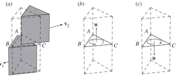
Figure 1.Mohr–Coulomb yield criteria: (a) yielding discontinuity between two rigid blocks showing normal forceN, resultant shear forcePand its componentsSandT; (b) conic yield surface whereNˆis the normal axis (tension positive) andˆSandTˆ

are orthogonal shear axes. The displacement jump orthogonal to the yield surface is shown, wherenandpare the normal displacement and shear plastic multiplier, respectively.

and

P=S2_+T2_{, (2.2)}

wherecandφare the material cohesion and angle of shearing resistance andais the face area

of the discontinuity. HereN,S andT denote the normal force and shear traction components

along then,sandtaxes, respectively, andPis the maximum shear traction on the discontinuity,

as indicated infigure 1. Similarly, the associative flow rule for a Mohr–Coulomb material can be

expressed by equations (2.3) and (2.4)

ptanφ−n=0 (2.3)

and

p≥s2_+t2_{, (2.4)}

where n, s andt denote the component of the relative jump in displacement rate across the

discontinuity in then,sandtdirections, respectively, andpis a plastic multiplier, as indicated in

figure 1. (Note that henceforth, ‘energy dissipation’ and ‘displacement’ will be used as shorthand for ‘rate of energy dissipation’ and ‘rate of displacement’, respectively.) Using equation (2.4), it is now possible to formulate the problem as an SOCP problem.

In the formulation outlined earlier, individual three-dimensional elements of material are rigid, and not free to deform. It therefore seems natural to use a formulation where the problem is posed entirely in terms of discontinuities. The discontinuity layout optimization (DLO)

procedure, outlined for two-dimensional plane plasticity problems by Smith & Gilbert [11], is

posed entirely in terms of discontinuities, and its potential application to three-dimensional problems is therefore considered here. An advantage of DLO is that it can inherently model singularities, such as those that exist at the edge or corner of an indentor or foundation footing. Conversely, finite elements, both rigid and deformable, generally require refinement

of the mesh in the regions of singularities [12], or alternatively the use of higher order shape

functions [13] in order to obtain reasonable results. The aim of this paper is to develop a

4

rspa.r

oy

alsociet

ypublishing

.or

g

Pro

c

R

So

c

A

469:

20130009

...

3. Discontinuity layout optimization

(a) Background

DLO is a direct limit analysis method, which means that it can directly provide an estimate of the maximum load sustainable by a solid body, without intermediate calculation steps. DLO can be used to generate upper bound plasticity solutions and associated collapse mechanisms.

The DLO procedure for plane strain problems is outlined in figure 2. Firstly, the initial

problem is discretized using nodes distributed across the body under consideration. Potential

discontinuity lines (e.g. ‘slip-lines’), along which jumps in displacements d can occur, are set

up by linking each node to every other node, and optimization is used to identify the subset of discontinuities active in the critical failure mechanism. Provided a sufficiently large number of nodes are employed, this allows a very wide range of potential mechanisms to be considered.

For plane strain problems, the corresponding optimization problem is given in equations (3.1)– (3.5), posed entirely in terms of potential discontinuities [11],

minλfT_Ld= −fT_Dd+gTp, (3.1)

subject to

Bd=0, (3.2)

Np−d=0, (3.3)

fT_Ld=1 (3.4)

and p≥0. (3.5)

In equation (3.2), compatibility is enforced explicitly at each node via a suitable compatibility

matrixBcontaining direction cosines. Equation (3.3) enforces the flow rule on each discontinuity

by introducing a vector of plastic multiplierspand a suitable flow matrixN, while equation (3.4)

ensures the work done by the live loads (fL) equals unity (where here the term ‘live loads’ is taken

to encompass all loads that are to be varied as part of the optimization process). Equation (3.1) is

the objective function, where the goal is to obtain the minimum load factorλby minimizing the

work done by dead loads (fD) and internal plastic energy dissipationgTp(wheregcontains the

corresponding dissipation coefficients).

Linear programming is then used to obtain the minimum value ofλ, seeking the optimal values

of the problem variables indandp. The critical subset of potential discontinuities, defining the

critical mechanism, is also identified, as indicated infigure 2d.

In this formulation, various intersections between discontinuities (or ‘crossover points’) occur throughout the problem domain. However, the displacement along each discontinuity remains unchanged either side of a ‘crossover point’, and hence compatibility is inherently maintained.

(b) Three-dimensional formulation

In the following sections a three-dimensional formulation is developed, using a three-dimensional grid of nodes and polygonal discontinuities. While any simple polygonal shape, or combination of simple polygonal shapes, may be used for the discontinuities, triangular discontinuities provide the most flexibility and will be used in the numerical examples. However, for the sake of clarity when describing the method, discontinuities of both rectangular and triangular shape will

be used. In general, when using triangular discontinuities there will be a total ofn(n−1)(n−2)/6

potential discontinuities, wherenis the total number of nodes used to discretize the problem (cf.

a total ofn(n−1)/2 potential line discontinuities in a plane strain problem). As with plane strain

5

rspa.r

oy

alsociet

ypublishing

.or

g

Pro

c

R

So

c

A

469:

20130009

...

(a) (b) (c) (d)

Figure 2.Stages in DLO procedure, after [14]: (a) starting problem (surcharge applied to block of material close to a vertical edge); (b) discretization of domain using nodes; (c) interconnection of nodes with potential discontinuities; (d) identification of critical subset of potential discontinuities using optimization (giving the layout of slip-lines in the critical failure mechanism).

n_D

n_E nE

n_D

n_C n_B

n_A nA

n_B n_C

O A

B

C

D E

A¢

D¢ E¢

C¢

(a)

v_DE v_EA

v_AB

v_BC

v_CD (b)

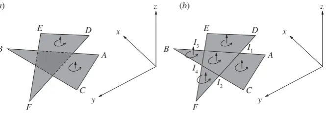
Figure 3.Solid bodies meeting at a common edge, (a) prior to, and (b) after movement, with prisms separated by discontinuities

−−→

OOXX, whereX=A,B. . .E. For clarity,Ohas not been shown, but lies in the planeABCDE.

(i) Compatibility

In plane strain DLO, compatibility is enforced at nodes. In three-dimensional DLO, compatibility

is conveniently enforced along shared edges.Figure 3shows a set of triangular prisms sharing

a common edge OO and with absolute displacements,vAB tovEA. The prisms are separated

by rectangular discontinuities OOXX, whereX=A, B. . .E. Each discontinuity OOXX has

a normal nX and a relative displacement jump vX that denotes the difference in absolute

displacement of the prisms meeting at this discontinuity. It follows from this definition that

equation (3.6), which involves summing all relative displacement jumps around edgeOO, must

hold

(vEA−vAB)+(vAB−vBC)+(vBC−vCD)+(vCD−vDE)+(vDE−vEA)=0. (3.6)

A sign convention for determining the directions ofn_Aton_Eandv_Atov_Eis presented in

appendix A. Using this sign convention and the vertex ordering infigure 3b, the following must

also be true along edgeOO:

vA+vB+vC+vD+vE=0. (3.7)

Compatibility can be similarly enforced along the remaining edges, using the sign convention given in appendix B. Moreover, equation (3.7) can be reformulated for each edge. Before

proceeding, it is first necessary to use coordinate systems local to each discontinuityi

6

rspa.r

oy

alsociet

ypublishing

.or

g

Pro

c

R

So

c

A

469:

20130009

...

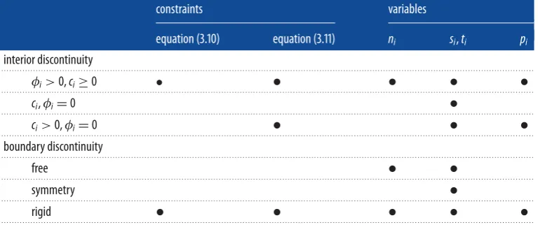
Table 1.Discontinuity flow rule conditions: applicable constraints and variables.

constraints variables

equation (3.10) equation (3.11) ni si,ti pi

interior discontinuity

. . . .

φi>0,ci≥0 •

•

•

•

•

. . . .

ci,φi=0

•

. . . .

ci>0,φi=0

•

•

•

. . . .

boundary discontinuity

. . . .

free

•

•

. . . .

symmetry

•

. . . .

rigid

•

•

•

•

•

. . . .

where T_i is a 3×3 transformation matrix converting local to global displacement jumps. T_i

is chosen such that one axis aligns with n_i, the unit column vector in the normal direction

using the ‘right-hand screw rule’; the two remaining orthogonal axes,s_iandt_i, are in the plane

of discontinuity i such thatT_i= {n_is_it_i}. Alsod_i= {nisiti}T, where ni, si and ti are the local

displacement jumps across discontinuityiin then_i,s_iandt_idirections, respectively. Compatibility can now be enforced for each edgej(j=1, 2,. . .,l) as follows:

i∈Sj

B_ijd_i=0, (3.9)

where Sj is a subset of the total number of discontinuitiesmthat contains the discontinuities

meeting at edgej, andB_ijis a local compatibility matrix equal tokijTi, wherekij is defined in

appendix B.

The DLO procedure results in intersections and overlaps between discontinuities that do not coincide with nodal connections; however, compatibility at these is enforced implicitly, as demonstrated in appendix C.

(ii) Flow rule

The local coordinate system described allows the associative flow rule for a Mohr–Coulomb material to be enforced using equations (2.3) and (2.4). Taking advantage of SOCP, the flow rule

on a discontinuityican be restated as follows:

pitanφi−ni=0 (3.10)

and

pi≥

s2

i +t2i, (3.11)

where pi is a plastic multiplier and where φi is the angle of friction on discontinuity i.

Equation (3.10) is a linear constraint and equation (3.11) is a second-order cone. In matrix form, equation (3.10) can be stated as follows:

Np−dn=0, (3.12)

wherednis a subset ofdcontaining only the displacement jumps normal to discontinuitiesi(i=

1,. . .,m),p is a global vector containing plastic multipliers andm is now the total number of

discontinuities in the problem.N is a globalm×m matrix enforcing the flow rule and equal

to diag(tanφ1, tanφ2,. . ., tanφm). However, depending on the material properties, it may not be

7

rspa.r

oy

alsociet

ypublishing

.or

g

Pro

c

R

So

c

A

469:

20130009

...

(iii) Dissipation function

The energy dissipated on a given discontinuity i is given by gipi, where gi is a dissipation

coefficient equal to_icda, the integral of the cohesive strength over the areaaof discontinuityi.

In the case of uniform cohesive strength across discontinuityi, the dissipation coefficientgi=aici,

whereaiandciare, respectively, the area and cohesion of the discontinuity.

On overlapping regions, the upper bound status of the solution is maintained, as demonstrated in appendix C.

(c) Mathematical formulation

A three-dimensional kinematic formulation for a cohesive-frictional body discretized using m

polygonal discontinuities andledges can be summarized as follows:

minλfT_Ld= −fT_Dd+gTp, (3.13)

subject to

Bd=0, (3.14)

Np−d_n=0, (3.15)

fT_Ld=1 (3.16)

and pi≥

s2

i +t2i ∀i∈ {1,. . .,m}, (3.17)

wherefD andfL are vectors containing, respectively, the specified dead and live loads. Hered

contains displacement jumps across the discontinuities,dT= {n1,s1,t1,n2,s2,t2,. . .,tm}, whereni

is the displacement jump normal to discontinuityi,siandtiare the displacement jumps within

the plane of discontinuityiandgis a vector of dissipation coefficients. HereBis a suitable 3l×3m

compatibility matrix,Nis a suitablem×mflow matrix anddn(a subset ofd) is a vector containing

the normal displacement jumps,dT_n= {n1,n2,. . .,nm}. Alsop is a vector of plastic multipliers,

pT= {p1,p2,. . .,pm}, wherepiis the plastic multiplier for discontinuityigiven by equation (3.17).

The optimization variables are the displacement jumps ind(anddn) and the plastic multipliers

inp. The objective function and the first three constraints are linear. The final constraints on the

plastic multipliers pi are second-order cones, so that the formulation is amenable to solution

using SOCP. The problem can also be posed in an equilibrium form, established using duality principles [15].

(d) Boundary conditions and loads

Many common boundary conditions can readily be modelled simply by using a reduced number

of variables and constraints, as indicated in the second half oftable 1. This for example shows that

a discontinuity on a rigid boundary is dealt with in exactly the same manner as a discontinuity in the interior of a domain.

Dead and live loads fT_D and fT_L in equations (3.13) and (3.16) are now defined such that

fT_D= {fn

D1,fD1s ,fD1t ,fD2n ,. . .,fDtm}andfTL= {fLn1,fLs1,fL1t ,fL2n,. . .,fLtm}, wherefDni,fDsi,fDtiandfLni,fLsi,fLti

are, respectively, the dead and live loads acting in theni,siandtidirections on discontinuityi.

Areas of flexible loading can be applied directly to the discontinuities with no special treatment. Rigid loads can be applied using a discontinuity covering the whole loaded area and reducing the degrees of freedom of underlying discontinuities appropriately.

At an external boundary, after taking account of any overlapping regions, displacement jumps

must equal the absolute displacement of that boundary. Hencef_Di andf_Liare simply the local

dead and live loads, respectively, on discontinuity i, resolved in the direction defined by the

local coordinate system when applied at boundary discontinuityi. For discontinuities within a

body, the contents off_Di andf_Li can be obtained by summing up the total overlying dead or

8

rspa.r

oy

alsociet

ypublishing

.or

g

Pro

c

R

So

c

A

469:

20130009

...

self weight only, and assuming this is applied in the negativezdirection, the contribution to the

summation made by discontinuityiis as follows:

fT_Did_i=W_id_i, (3.18)

whereW_iis a 1×3 row vector containing the components in then_i,s_iandt_idirections of the total

weight of the column lying vertically above discontinuityi.

(e) Summary of procedure

Steps in the DLO procedure for three-dimensional problems can be summarized as follows:

— discretize the problem using nodes; — connect nodes to create edges;

— join edges to create polygonal discontinuities; — set-up problem, using equations (3.13)–(3.17); and — solve the resulting SOCP problem.

4. Numerical examples

To evaluate the potential of the method, various three-dimensional examples are now considered. Unless stated otherwise, all computations were performed using a workstation equipped with 2.6 GHz AMD Opteron 6140 processors, 8 GB RAM and running 64 bit Scientific Linux.

The MOSEKinterior-point solver with SOCP capability was used [16]. The default settings of

the optimizer were used, including the pre-solve feature. The CPU times reported are for the optimizer only, including the time taken for the pre-solve routine to execute, but excluding the time taken to read in and set up a given problem.

Prior to solving, various measures were taken to condition and/or reduce the size of a given problem. Firstly, the coefficients in the objective function (3.13) and unit displacement constraint (3.16) were scaled as necessary to ensure the problem was well posed. Secondly, as overlapping edges do not provide any extra degrees of freedom, these were removed. Thirdly, discontinuities covering areas that could be reconstructed by combining several discontinuities covering smaller areas were removed. Fourthly, noting that the formulation naturally results in

3(n−1) linear dependencies in the constraint matrix, wherenis the total number of nodes, such

linear dependencies were identified and removed prior to passing the problem to the optimizer. Lastly, while the basic DLO procedure involves positioning nodes on a Cartesian grid, the use of other nodal arrangements is possible, and, where clearly indicated, regular grids with differing

x,yandzspacings are used in this paper. However, it should be noted that an adaptive solution

procedure capable of dramatically reducing problem size (e.g. of the sort described in [11] for

plane strain problems) was not used in the numerical studies described herein. Thus the size of a problem increases rapidly as nodal resolution is increased, and consequently only relatively small problems are considered here.

(a) Compression of a block

The unconfined compression of a square block with shear strength parametersc,φbetween two

perfectly rough rigid platens has previously been considered by Martin & Makrodimopoulos

[8], who have obtained upper and lower bound solutions for this problem. This problem will

therefore be used as a benchmark for the proposed three-dimensional DLO procedure. For the

geometry shown infigure 4, the objective is to find the ratio of the average bearing pressureqto

cohesive shear strengthc.

Symmetry means that only 1/16 of the block needs to be modelled, as indicated infigure 4.

Nodes were initially positioned on a Cartesian grid (i.e. equal nodal spacings in thex,yandz

9

rspa.r

oy

alsociet

ypublishing

.or

g

Pro

c

R

So

c

A

469:

20130009

...

2

2 1

z

x y

Dz

Dy

Dx

Figure 4.Compression of a block: problem geometry, nodal spacings (x,yandz) and the 1/16 of the volume modelled, owing to symmetry.

Table 2.Compression of a block: comparison with benchmark solutions. Upper bound (UB) solutions from Martin & Makrodimopoulos [8] have been used to benchmark the present solutions, and their lower bound (LB) solutions are also listed for information;=x=y=z.

benchmark discontinuities

φ(◦) UB LB spacing total no. active (%) solution difference (%) CPU (s)

0 2.305 2.230 ₄1 7704 2.7 2.319 0.60 12

. . . .

1

6 117 936 2.7 2.314 0.39 9700

. . . .

30 10.06 8.352 1

4 7704 10 12.48 18 2.0

. . . .

1

6 117 936 4.0 11.69 10 5000

. . . .

For φ=0◦, the best new solution presented is close (within 0.39%) to the benchmark upper

bound solutions of Martin & Makrodimopoulos [8]. A representative collapse mechanism is

shown infigure 5. In the case ofφ=30◦, the best new solution compares less favourably with

the benchmark (difference 10%).

Noting that the active discontinuities infigure 5radiate from the centre, it is of interest to

investigate the effect of using different nodal spacings in thexdirection compared with those

in theyandzdirections. Results for theφ=0◦case for various nodal spacings are presented in

table 3.

Firstly, it is evident that a solution matching the best reported value of 2.314 presented previously could be obtained in only 0.22 s, compared with 9700 s previously. This is because only a small subset of the discontinuities present previously are now included. Secondly, it is evident that it has been possible to improve on the benchmark upper bound solution (the best DLO solution of 2.304 is slightly less than the value of 2.305 obtained by Martin &

Makrodimopoulos [8]).

(b) Punch indentation

The bearing capacity of a perfectly rough square indenter resting on the surface of a purely

cohesive Tresca material is now considered. The value of interest is once again the ratio q/c,

otherwise known as the bearing capacity factorNc. Salgadoet al.[17] have established upper and

lower bounds for a variety of indenter embedment depths and geometries using finite-element

limit analysis. Gourvenec et al.[18] have modified the upper bound mechanism proposed by

10

rspa.r

oy

alsociet

ypublishing

.or

g

Pro

c

R

So

c

A

469:

20130009

...

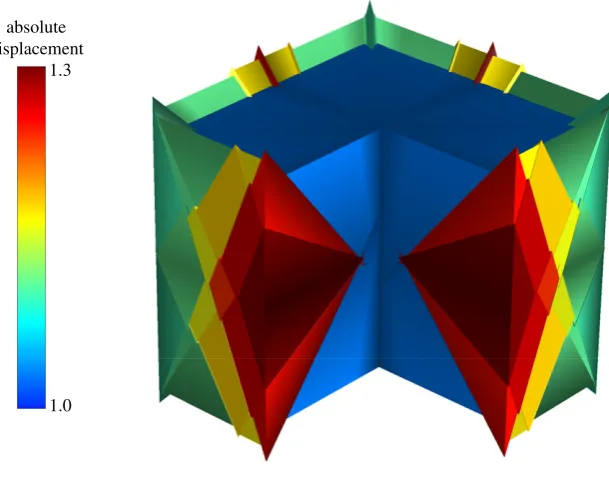
absolute displacement

1.3

1.0

Figure 5.Compression of a block: typical failure mechanism forφ=0 case (x,y,z=14).

Table 3.Compression of a block: use of different nodal grid spacings. Upper bound (UB) solutions from Martin & Makrodimopoulos [8] have been used to benchmark the present solutions, and their lower bound (LB) solutions are also listed for information;x=1.

benchmark discontinuities

φ(◦) UB LB spacingy,z total no. active (%) solution difference (%) CPU (s)

0 2.305 2.230 1₄ 356 29 2.319 0.60 0.04

. . . .

1

6 1500 30 2.314 0.39 0.22

. . . .

1

8 4452 26 2.309 0.18 1.9

. . . .

1

12 23 100 21 2.307 0.072 50

. . . .

1

18 133 884 16 2.304 −0.043 1800

. . . .

Table 4.Punch indentation: comparison with benchmark solutions. Upper bound (UB) solutions from Vicenta da Silva & Antão [21] have been used to benchmark the present solutions, and lower bound (LB) solutions from Salgadoet al. [17] are also listed for information.

benchmark discontinuities

UB LB spacing total no. active (%) solution difference (%) CPU (s)

6.051 5.52 1₂ 157 17 6.521 7.8 0.02

. . . .

1

4 7365 4.6 6.405 5.9 13

. . . .

1

6 114 310 1.6 6.226 2.9 6400

. . . .

[20] and Vicente da Silva & Antão [21] have also established upper bounds for a number of

indenter geometries bearing onto the material surface. The best reported upper and lower bounds

for a square indenter are included intable 4.

The problem geometry used is shown infigure 6. While both Michalowski [20] and Gourvenec

11

rspa.r

oy

alsociet

ypublishing

.or

g

Pro

c

R

So

c

A

469:

20130009

...

1

1

2 2

1 2

z

x y

D D

D

Figure 6.Punch indentation: problem geometry, nodal spacing, and the 1/8 of the volume modelled, owing to symmetry.

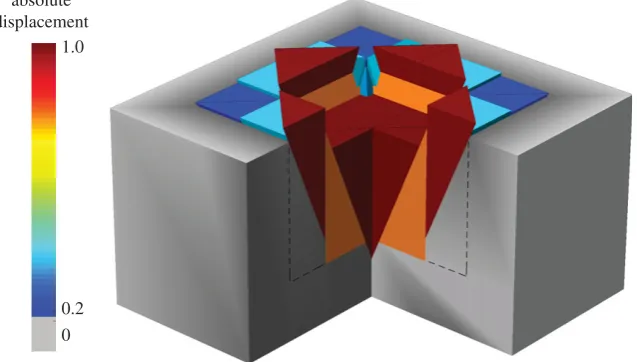
absolute displacement

1.0

0.2 0

Figure 7.Punch indentation: representative failure mechanism (=1/2,φ=0) (dashed lines indicate extent of domain modelled).

bound solutions, owing to Vicente da Silva & Antão [21] and Salgadoet al.[17], respectively, have taken advantage of the four planes of symmetry inherent in the problem geometry. Therefore, only

1/8 of the problem has been modelled, as indicated infigure 6.Table 4presents new solutions for

three nodal spacings, with all nodes positioned on a Cartesian grid (i.e. equal nodal spacings

in thex,yandzdirections). These solutions compare well with the best reported upper bound,

especially considering the comparatively low nodal resolutions employed. Also, following the initial study, access to a workstation with 16 GB RAM allowed consideration of a finer numerical

discretization (with=1/8), resulting in an improvedNc=6.102 (difference 0.84%).

A representative failure mechanism is shown infigure 7. It should be noted that the critical

mechanisms for all three nodal grids extend up to the fixed boundaries. However, extending the problem domain relative to the foundation quickly leads to impractically large problem sizes, so this issue was not investigated further.

(c) Anchor in a purely cohesive soil (

φ

=

0)

Consider a perfectly rough anchor of widthBembedded at a depthHin a purely cohesive Tresca

soil, as shown infigure 8. Immediate breakaway (i.e. no suction or transmission of tensile stresses)

12

rspa.r

oy

alsociet

ypublishing

.or

g

Pro

c

R

So

c

A

469:

20130009

...

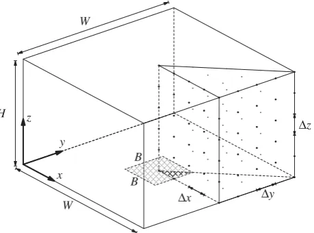
B

B

Dx Dy

Dz z

x y

W

W H

Figure 8.Anchor: problem geometry, nodal spacings (x,yandz) and the 1/8 of the volume modelled, owing to symmetry.

problem needs to be modelled, as shown infigure 8. VariousH/Bratios have been considered by

fixingB=2,W=10,x=y=1,z=H/4 and varyingH.

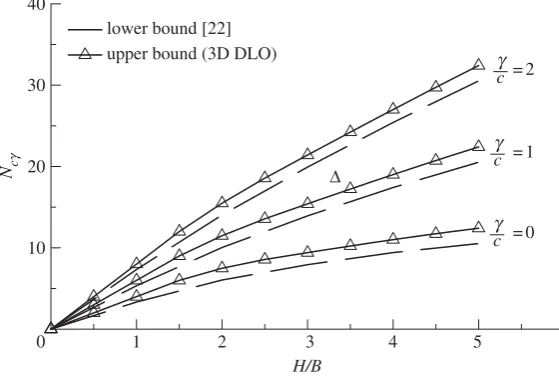
Merifieldet al.[22] used a lower bound finite-element limit analysis procedure to establish

bounds on the break-out factor at various embedment depths. The break-out factorNc0 for an

anchor in a weightless cohesive soil is defined as average bearing pressureq divided by the

cohesive strengthc. For a soil with unit weightγ, Merifieldet al.[22] defined the break-out factor

Ncγ as

Ncγ=Nc0+γH

c . (4.1)

Failure mechanisms can be classified as ‘shallow’, where the failure mechanism extends up from the anchor to the soil surface, and ‘deep’, where the mechanism involves only localized

deformations around the anchor, and where the break-out factor Nc∗ is independent of the

embedment depthH. For a given ratioγ /c, the deep mechanism becomes critical at depths greater

than or equal toHcr. If both deep and shallow mechanisms are considered,Ncγ must be less than

or equal toNc∗. Merifieldet al.[22] established a lower bound onNc∗≈11.9. Forγ /c=0, Merifield

et al.[22] foundHcr≈7.

Figure 9 shows break-out factors for shallow failures at various embedment depths. These

show good agreement with those reported by Merifieldet al. [22] whenγ /c=0 and H<Hcr.

Furthermore, the results forγ /c=1 andγ /c=2 are consistent with the relationship described

in equation (4.1). The mechanisms developed did not extend to the lateral fixed boundary,

suggesting thatNcandNcγ were not influenced by the extent of the domain modelled.

(d) Anchor in a purely frictional soil

Now consider a perfectly rough anchor of widthBembedded at depthHin a purely frictional

soil with an angle of shearing resistanceφ=30◦and a unit self weightγ. Assuming an associative

flow rule, only mechanisms that extend to the surface are possible. The break-out factorNγ in this

case can be expressed as

Nγ =_γq

H (4.2)

whereqis the average pressure on the anchor. Merifieldet al.[23] used a lower bound

finite-element analysis procedure to establish bounds on the break-out factor for various angles of

13

rspa.r

oy

alsociet

ypublishing

.or

g

Pro

c

R

So

c

A

469:

20130009

...

Nc

g

H/B

0 1 2 3 4 5 6

10 20 30 40

c =2

D

g

cg =1

c =0 g lower bound [22]

upper bound (3D DLO)

Figure 9.Anchor: cohesive soil break-out factors.

Ng

0 10 20

H/B

upper bound f=30°[24] lower bound f=30° [23]

upper bound f=30° (3D DLO GRID 1) upper bound f=30° (3D DLO GRID 2)

1 2 3 4 5 6

Figure 10.Anchor: frictional soil break-out factors using nodal grids GRID 1 and GRID 2.

given in equation (4.3), obtained by assuming a simple rigid block mechanism,

Nγ=1+H

B tanφ

2+π

3Htanφ

. (4.3)

Using nodal grids of the form shown in figure 8and fixing B=2,W=10,x=y=1,z=

H/4 (denoted GRID 1) and varying H, a very close fit to equation (4.3) has been found for

0.5≤H/B≤2.5 (figure 10). Above this range, the mechanism reaches the lateral fixed boundary

and no solution was obtained. The critical mechanism is relatively simple, and very similar results

can be obtained using an alternative grid, whereB=2,W=16,x=y=1,z=H (denoted

GRID 2). GRID 2 also has been used to determineNγ for 2.5<H/B≤5, which also compare well

14

rspa.r

oy

alsociet

ypublishing

.or

g

Pro

c

R

So

c

A

469:

20130009

...

5. Discussion

As can be seen in §4, the three-dimensional DLO procedure is capable of obtaining results comparable with those found in the literature. Also in one case an improved upper bound solution was found. A key benefit of the procedure is that it can automatically identify traditional ‘upper bound’ mechanisms, obviating the need for these to be found manually, as has hitherto been necessary. Such mechanisms are generally easy to visualize and can be checked by hand if required. Thus, a potentially useful application of the method is in helping designers identify critical mechanisms for subsequent use in hand calculations. While only translational mechanisms are currently identified, experience gained applying plane strain DLO to practical problems has indicated that solutions of acceptable accuracy for engineering purposes can often be obtained, even for problems where rotational modes are critical. Additionally, mechanisms that include continuous deformations can be captured by using high concentrations of active discontinuities.

However, refining the nodal grid even slightly leads to a large increase in the number of potential discontinuities, which means that problems can quickly become impractically large using currently available computational power. Thus enhancements to improve performance are required. One potential approach is to implement an adaptive solution procedure, similar to that

proposed for plane strain problems by Smith & Gilbert [11]. With the latter procedure a subset

of the total number of potential discontinuities is used in the initial optimization. The solution is then assessed, and discontinuities deemed most likely to improve it are added. A further optimization is then performed and the process repeated until a rigorous termination criterion is met, ensuring that the numerical solution is the same as would have been obtained had all potential discontinuities been included in the optimization at the outset. For all problems considered in this paper, the percentage of discontinuities with non-zero displacements was small, suggesting that a similar adaptive solution procedure might be effective, ensuring that the number of discontinuities modelled in the optimization problem is kept to a minimum. Developing such a procedure is therefore a topic for future research.

6. Conclusions

— A new three-dimensional plasticity formulation has been described. The formulation uses the DLO procedure to directly identify critical translational collapse mechanisms. Planar triangular discontinuities, which interconnect nodes distributed across the domain, are employed and SOCP is used to identify the optimal subset of discontinuities, which define the geometry of the collapse mechanism.

— A key benefit of the DLO procedure is that it can automatically identify traditional ‘upper bound’ collapse mechanisms, obviating the need for these to be found manually, as has hitherto been necessary.

— Despite the use of comparatively coarse nodal discretizations, reasonably good correlation with literature benchmark solutions has been observed. Furthermore, the best upper bound solution for the compression of a purely cohesive block between two perfectly rough platens problem reported in the literature has been improved upon. — The use of an adaptive solution procedure, similar to that successfully used in plane strain

DLO, is likely to allow finer nodal discretizations to be treated. This has therefore been identified as a topic for future research.

Appendix A. Sign convention

In DLO, the optimization problem is formulated purely in terms of displacement jumps across a set of potential discontinuities. This requires a consistent sign convention to be adopted.

Figure 11ashows two triangular prisms separated by a discontinuityABCmoving with absolute

15

rspa.r

oy

alsociet

ypublishing

.or

g

Pro

c

R

So

c

A

469:

20130009

...

v₂

v₁

A

B _C

(a)

n

A

B _C

(b)

n

A

B _C

(c)

Figure 11.Sign convention: (a) two triangular prisms separated by a discontinuityABC, the dashed outline shows the original positions of the prisms; (b) discontinuity vertex ordering−→ABC; (c) discontinuity vertex ordering−ACB→.

must equal either v1−v2 orv2−v1. Using the ‘right-hand screw rule’, the normaln to the

discontinuity can be determined for a particular ordering of the vertices, as demonstrated in

figure 11b,cfor discontinuityABC.v_ABCis simply defined asv₊−v₋, wherev₊andv₋are the

velocities of the blocks on thenpositive andnnegative sides of the discontinuity, respectively,

for the chosen ordering of the vertices.

Appendix B. Convention for selecting the vertex ordering parameter

_k

_ij

A sign convention is necessary for equations (3.7) and (3.9) to be valid along edge j (where

j=1, 2,. . .,land wherelis the total number of edges used to discretize the problem). Taking

account of the sign convention, these equations can be rewritten as follows:

i∈Sj

kijvi=0 (B 1)

and

i∈Sj

kijTidi=

i∈Sj

B_ijd_i=0, (B 2)

whereSjis the subset of all discontinuities meeting at edgej.kij= ±1 depends on the relative

vertex orderings of discontinuityiand edgej.

Each discontinuityi(i=1, 2,. . .,m) is defined by a subsetDiof the total nodesn, wheremis the

total number of discontinuities andDicontains the vertices of discontinuityi. Discontinuityihas a

boundary formed by a subsetKiof the total number of edgesl. Each edgej(j=1, 2,. . .,l) is defined

by subsetEjof the total nodesn, whereEjcontains the two vertices of edgej. The following is

a suitable convention for selectingkijfor all edgesj(j=1, 2,. . .,m) and all discontinuitiesi(i=

1, 2,. . .,m).

(i) For each discontinuityi(i=1, 2,. . .,m), define a positive ordering of the vertices inDi.

The two vertices of each edgej(j∈Ki) must be adjacent in this ordering. The ordering

defined is cyclical (i.e. the first vertex is adjacent to the last) and is also used to definen_i

(see appendix A).

(ii) For each edgej(j=1, 2,. . .,l), define a particular ordering of the verticesEjas positive.

(iii) For each edgej(j=1, 2,. . .,l) and discontinuityi(i∈Sj) with common vertices{X,Y} =

Di∩Ej, compare the orderings ofXandYin the positive orderings ofEjandDidefined

in (i) and (ii), respectively, noting that the ordering ofDiin (i) is cyclical. If these orderings

16

rspa.r

oy

alsociet

ypublishing

.or

g

Pro

c

R

So

c

A

469:

20130009

...

D C

B

A

E F G

H

(a)

D C

B

A

E F G

H

I₃ I₄ I₅

I₁ I₂ I₆

(b)

Figure 12.Crossovers: (a) discontinuity−→ABCD, displacement jumpv_ABCD, intersecting discontinuity−→EFGH, displacement jump

vEFGH; (b)−→ABCDsplit into−−→ABI2I1and−−→I1I2CD, both with a displacement jumpvABCD;−→EFGHsplit into−−→I1I2I6I5,−−→I3I4I2I1,−−−→EI3I1I5Hand

−−−→

I4FGI6I2, all with a displacement jumpvEFGH.

Appendix C. Crossovers and overlaps

(a) Crossovers

Intersections between discontinuities can occur, much as in plane strain DLO problems. The intersections between discontinuities on different planes are line segments or ‘crossovers’. Compatibility is implicitly ensured at these crossovers rather than being explicitly enforced. This can be demonstrated using the two intersecting rectangular discontinuities, as shown in

figure 12a. In figure 12b, the discontinuities are split into smaller discontinuities so that the crossover is eliminated. In DLO, it is assumed that the displacement jump across each of these smaller discontinuities is equal to that of its parent, taking account of the conventions in appendices A and B. It is clear that equation (B 1) is satisfied for the new edges and the original crossover itself must also be compatible.

(b) Overlaps

Intersections also occur between discontinuities in the same plane, resulting in ‘overlaps’. As

with crossovers, compatibility is implicitly ensured. Infigure 13a, two overlapping discontinuities

are shown. These are divided in figure 13b so that the original overlap is eliminated, but

two overlapping discontinuities −−−−→I1I3I4I2ABC and−−−−→I1I3I4I2DEF remain. Discontinuities located on

different planes and sharing edges AB, BC, EF and FD are similarly divided (not shown

in figure 13). The displacement jump for each new discontinuity equals that of its parent discontinuity, taking account of the conventions in appendices A and B. Using equation (B 1),

it is simple to prove that compatibility is maintained and that the displacement jumpv_Ion the

overlapping regionI1I3I4I2equalsvABC+vDEF.

CalculatingpABC,pDEFandpIfrom equation (3.11), it is clear thatpABC+pDEF≥pIsince these

terms are not added vectorially in the SOCP solver. It can therefore be concluded that overlaps will overestimate both the dilation and energy dissipated. This is equivalent to the overlapping

region having a cohesive strength c and angle of frictionφ greater than those of the original

17

rspa.r

oy

alsociet

ypublishing

.or

g

Pro

c

R

So

c

A

469:

20130009

...

x

y

z

A

C B

D E

F

(a) (b)

x

y

z

A

C B

D E

F I₃

I₄ I₂

I₁

Figure 13.Overlaps: (a) a discontinuity−→ABC, displacement jumpv_ABC, overlapping a discontinuity−DEF→, displacement jump

vDEF; (b)−→ABCsplit into−−→AI1I2C,−−→I1I3I4I2ABCand−→I3BI4, each with a displacement jumpvABC;−DEF→split into−−→DEI3I1,−−→I1I3I4I2DEFand

−→

I2I4F, each with a displacement jumpvDEF.

tend to avoid such overlaps where these result in more energy being dissipated than necessary. Therefore, the significance of these overlaps is likely to reduce with increasing nodal resolution.

The load distribution across discontinuitiesABCandDEFis unknown and can be interpreted

in any manner consistent with the work done by vABC,vDEF andvI. Note that the load

on I1I3I4I2,LI, cannot be the sum of the loads on −−−−→I1I3I4I2ABC and−−−−→I1I3I4I2DEF, LABC_I andLDEF_I ,

respectively (i.e.LI=LABC_I +LDEF_I ). Load distributions resulting inLI=LABC_I =LDEF_I will always

be consistent with the work done.

References

1. Lysmer J. 1970 Limit analysis of plane problems in soil mechanics.J. Soil Mech. Found. Div.

ASCE96, 1311–1334.

2. Sloan SW. 1988 Lower bound limit analysis using finite elements and linear programming.

Int. J. Numer. Anal. Methods Geomech.12, 61–77. (doi:10.1002/nag.1610120105)

3. Makrodimopoulos A, Martin CM. 2006 Lower bound limit analysis of cohesive-frictional

materials using second-order cone programming.Int. J. Numer. Methods Eng. 66, 604–634.

(doi:10.1002/nme.1567)

4. Park JJ, Kobayashi S. 1984 Three-dimensional finite element analysis of block compression.

Int. J. Mech. Sci.26, 165–176. (doi:10.1016/0020-7403(84)90051-1)

5. Lyamin AV, Sloan SW. 2002 Lower bound limit analysis using non-linear programming.Int. J.

Numer. Methods Eng.55, 573–611. (doi:10.1002/nme.511)

6. Lyamin AV, Sloan SW. 2002 Upper bound limit analysis using linear finite elements and

non-linear programming.Int. J. Numer. Anal. Methods Geomech.26, 181–216. (doi:10.1002/nag.198)

7. Krabbenhøft K, Lyamin AV, Sloan SW. 2008 Three-dimensional Mohr–Coulomb limit analysis

using semidefinite programming.Commun. Numer. Methods Eng.24, 1107–1119. (doi:10.1002/

cnm.1018)

8. Martin C, Makrodimopoulos A. 2008 Finite-element limit analysis of Mohr–Coulomb

materials in 3D using semidefinite programming.J. Eng. Mech.134, 339–347. (doi:10.1061/

(ASCE)0733-9399(2008)134:4(339))

9. Chen J, Yin J, Lee CF. 2003 Upper bound limit analysis of slope stability using rigid elements

and nonlinear programming.Can. Geotech. J.40, 742–752. (doi:10.1139/T03-032)

10. Alizadeh F, Goldfarb D. 2003 Second-order cone programming.Math. Program. Ser. B95, 3–51.

(doi:10.1007/s10107-002-0339-5)

11. Smith C, Gilbert M. 2007 Application of discontinuity layout optimization to plane plasticity

problems.Proc. R. Soc. A463, 2461–2484. (doi:10.1098/rspa.2006.1788)

12. Lyamin AV, Sloan SW, Krabbenhøft K, Hjiaj M. 2005 Lower bound limit analysis with adaptive

remeshing.Int. J. Numer. Methods Eng.60, 1961–1974. (doi:10.1002/nme.1352)

13. Makrodimopoulos A, Martin CM. 2007 Upper bound limit analysis using simplex strain

elements and second-order cone programming. Int. J. Numer. Anal. Methods Geomech. 31,

18

rspa.r

oy

alsociet

ypublishing

.or

g

Pro

c

R

So

c

A

469:

20130009

...

14. Gilbert M, Smith C, Haslam I, Pritchard T. 2010 Application of discontinuity layout

optimization to geotechnical limit analysis problems. InProc. 7th European Conf. Numerical

Methods Geotechnical Eng.(NUMGE), Trondheim, Norway(eds T Benz, S Nordal), pp. 169–174. CRC Press.

15. Boyd S, Vandenberghe L. 2004Convex optimization. Cambridge, UK: Cambridge University

Press.

16. Mosek. 2011TheMOSEKoptimization tools manual. Seehttp://www.mosek.com. Copenhagen,

Denmark: Mosek ApS.

17. Salgado R, Lyamin AV, Sloan SW, Yu HS. 2004 Two and three-dimensional bearing capacity of

foundations on clay.Géotechnique54, 297–306. (doi:10.1680/geot.2004.54.5.297)

18. Gourvenec S, Randolph M, Kingsnorth O. 2006 Undrained bearing capacity of square and

rectangular footings.Int. J. Geomech.6, 147–157. (doi:10.1061/ASCE1532-3641(2006)6:3(147))

19. Shield RT, Drucker DC. 1953 The application of limit analysis to punch-indentation problems.

J. Appl. Mech.20, 453–460.

20. Michalowski RL. 2001 Upper-bound load estimates on square and rectangular footings.

Géotechnique51, 787–798. (doi:10.1680/geot.2001.51.9.787)

21. Vicente da Silva MV, Antão AN. 2008 Upper bound limit analysis with a parallel mixed finite element formulation.Int. J. Solids Struct.45, 5788–5804. (doi:10.1016/j.ijsolstr.2008.06.012) 22. Merifield RS, Lyamin AV, Sloan SW, Yu HS. 2003 Three-dimensional lower bound

solutions for stability of plate anchors in clay. J. Geotech. Geoenviron. Eng. 129, 243–253.

(doi:10.1061/(ASCE)1090-0241(2003)129:3(243))

23. Merifield RS, Lyamin AV, Sloan SW. 2006 Three dimensional lower-bound solutions for the

stability of plate anchors in sand.Géotechnique56, 123–132. (doi:10.1680/geot.2006.56.2.123)

24. Murray EJ, Geddes JD. 1987 Uplift of anchor plates in sand. J. Geotech. Eng.113, 202–215.