Scale-invariant moving finite elements for nonlinear partial differential equations in two dimensions

This is a repository copy of Scale-invariant moving finite elements for nonlinear partial differential equations in two dimensions.

White Rose Research Online URL for this paper: http://eprints.whiterose.ac.uk/1784/

Article:

Baines, M.J., Hubbard, M.E., Jimack, P.K. et al. (1 more author) (2006) Scale-invariant moving finite elements for nonlinear partial differential equations in two dimensions. Applied Numerical Mathematics, 56 (2). pp. 230-252. ISSN 0168-9274

https://doi.org/10.1016/j.apnum.2005.04.002

[email protected] https://eprints.whiterose.ac.uk/ Reuse

See Attached

Takedown

If you consider content in White Rose Research Online to be in breach of UK law, please notify us by

White Rose Consortium ePrints Repository

This is an author produced version of a paper published in Applied Numerical

Mathematics.

White Rose Repository URL for this paper: http://eprints.whiterose.ac.uk/1784/

Published paper

Baines, M.J., Hubbard, M.E., Jimack, P.K. and Jones, A.C. (2006)

Scale-invariant moving finite elements for nonlinear partial differential equations in two dimensions. Applied Numerical Mathematics, 56 (2). pp. 230-252.

Scale-Invariant Moving Finite Elements for

Nonlinear Partial Differential Equations in

Two Dimensions

M.J. Baines

M.E. Hubbard

P.K. Jimack

A.C. Jones

a_{Department of Mathematics, The University of Reading, UK}

b_{School of Computing, University of Leeds, UK}

Abstract

A scale-invariant moving finite element method is proposed for the adaptive solution of nonlinear partial differential equations. The mesh movement is based on a finite element discretisation of a scale-invariant conservation principle incorporating a monitor function, while the time discretisation of the resulting system of ordinary differential equations is carried out using a scale-invariant time-stepping which yields uniform local accuracy in time. The accuracy and reliability of the algorithm are successfully tested against exact self-similar solutions where available, and otherwise against a state-of-the-art h-refinement scheme for solutions of a two-dimensional porous medium equation problem with a moving boundary. The monitor functions used are the dependent variable and a monitor related to the surface area of the solution manifold.

Key words: scale invariance, moving meshes, finite element method, porous medium equation, moving boundaries

1 Introduction

reflect these scaling properties: scale invariance can then be used to define a time-step strategy which yields uniform local accuracy in time, as in [8].

A natural framework for the space discretisation is a moving mesh (see, for example, [2,5,10,11,15]). In this work the mesh will be coupled with the so-lution and moved at each time-step in such a way as to seek to conserve in time the scale-invariant integral of a monitor function, as distributed within each local patch of finite elements. It will be shown that this strategy can produce accurate results, even when the integral over the whole domain is not conserved exactly in time, provided that the dependent variable is recovered in an appropriate manner. The conservation principle can be interpreted as a fluid property (cf. the GCL method of [10]) and used in conjunction with the PDE to generate an equation for a velocity field which is a function of the space coordinate and time, as in [7]. The velocity field may then be integrated to obtain new mesh positions. The solution of the PDE can be reconstructed from the new mesh either directly from the conservation principle itself or from moving forms of the PDE. A similar approach has already been applied in [3] to a range of moving boundary problems in one and two space dimen-sions using the dependent variable as monitor function. This paper extends those results to include scale-invariant monitor functions, scale-invariant time-stepping, a surface area type monitor in 2D and more robust forms of solution recovery. The accuracy of the technique is assessed by comparison with gen-eral solutions of the porous medium equation obtained through an alternative numerical method, in addition to the similarity solutions used in [3].

The plan of the paper is as follows. In Section 2 the steps of the new method are summarised, prior to their detailed description in later sections. In Sec-tion 3 we discuss the principles of scale invariance as they apply to nonlinear PDEs. Next we recall in Section 4 how a given function can be well represented on an irregular mesh using an equidistribution principle. We then show how, as time evolves, the same principle, extended with the help of scale invari-ance, becomes a conservation principle governing the evolution of the mesh in time (cf. [11]). Weak forms of these principles are introduced with a view to constructing finite element approximations. In Section 5, in order to gen-erate an associated velocity field, the conservation principle is identified with a Lagrangian statement of conservation of mass for a fluid problem (cf. [10]). By transforming to an Eulerian frame via the Reynolds Transport Theorem and using the PDE we can obtain an equation for the corresponding Eulerian velocity field. Uniqueness is ensured by specifying the vorticity of the field, as in [10], thus introducing a velocity potential which satisfies an elliptic equa-tion. The velocity is integrated in time to give the new position of the moving coordinates. Weak forms of the derivation are also given in preparation for the application of finite elements.

velocity potential equations using standard linear finite elements. These linear elements are moved with a piecewise linear velocity field (which is formally a recovered gradient of a piecewise linear velocity potential) and carry with them a piecewise linear finite element solution. Section 7 is concerned with time-stepping. The finite element discretisation in space generates an ODE system for the nodal positions which is integrated in time using a scaled time variable which provides a scale-invariant local truncation error and hence, as in [8], a relative local truncation error which is uniformly accurate in time.

In Section 8 we discuss how the solution can be recovered from the nodal positions in three possible ways, (i) by inverting the conservation principle directly, (ii) by using an ALE (Arbitrary Lagrangian Eulerian) approach to the differential form of the PDE, or (iii) by using an ALE integral form of the PDE. Monitor functions are considered in Section 9. They are chosen here to be either the dependent variable itself or a surface area type monitor, but the approach is readily generalised to other monitors. In Section 10 the accu-racy and reliability of the algorithm is tested for the two-dimensional porous medium equation (PME), both against a range of known analytic similarity solutions and against results from a state-of-the-art h-refinement code. Each of the monitor functions is tested, along with the three different approaches to recovering the nodal solution values at each time-step, for a selection of PME problems. The paper concludes with a short discussion.

2 Overview of the proposed algorithm

In this section we rehearse the main steps of the new method before expand-ing on them in more detail. The first and pivotal step is the definition of a distributed conservation principle in a moving frame which depends on a time-dependent monitor function. Crucially this monitor function is constructed so that its integral is scale-invariant. The next step is to derive an equation for the velocity associated with this moving frame, carried out by differentiating the distributed conservation principle with respect to time, using the Reynolds Transport Theorem and incorporating the original PDE. This equation, which is actually a weak form of the PDE, is also scale invariant, as are all the equa-tions constructed here. A velocity potential is then introduced, based on the assumption of an irrotational velocity field, which satisfies an associated weak elliptic equation. Finally the velocity is recovered from the potential, using a weak form of their relationship, and integrated in time.

the finite element solution is completed by reconstructing the solution from the new mesh or its nodal velocities.

3 Scale invariance

Scale invariance is a natural property of models of physical systems due to their independence of physical units [4]. For a scale-invariant problem governed by the PDE

ut = Lu (1)

(whereLuis a purely spatial operator), together with properties conferred by the boundary conditions, there exist indices β and γ such that the scalings

t =λˆt , x=λβ_{xˆ, u=λ}γ_{u ,ˆ (2)}

leave the problem invariant (λ is simply an arbitrary scaling factor). For ex-ample, in the case of the porous medium equation in d dimensions,

ut = ∇ ·(un∇u) in Ω, (3)

subject tou|∂Ω= 0 (which enforces conservation of mass) it can be shown [4]

thatβ = 1/(nd+ 2) and γ =−d/(nd+ 2). For this problem there exist known self-similar solutions with compact support and a moving boundary, see for example [16], which represent intermediate asymptotic solutions in the sense of [4].

4 Equidistribution, monitor functions and conservation

Given an initial conditionu=u0for equation (1) and a non-negative, solution-dependent monitor functionm(u), the basic form of an equidistribution prin-ciple is

mave(u0) ∆Ω = c0, (4)

where ∆Ω is the size (area in 2D) of a subregion of the total domain Ω,mave

is an average ofm over this subregion, andc0 is a constant, determined by the problem. The principle (4) associates small subregions with large values ofm

large. (For exposition purposes the monitor function m is taken here to be a function of u only, although the analysis in this paper is readily extended to monitors which are functions of derivatives of u: indeed, one of the monitor functions that we shall use depends upon the gradient of u.)

In the present work we are interested in maintaining such a distribution in time. It will be assumed here that the initial mesh already has a desired distribution of the monitor, i.e.

mave(u0) ∆Ω = c∆Ω, (5)

wherec∆Ωis a constant associated with the subregion ∆Ω and determined by

the initial conditions.

It is not generally possible to maintain the same distribution principle on a moving mesh as time progresses. A similar distribution may still exist at later times, but constants different to c∆Ω will arise unless mave(u) ∆Ω(t) remains

constant in time. However, if the PDE problem is scale-invariant, with scaling exponentsβ and γ as in equation (2), we may define a time-dependent scaled monitor function ˜m(t, u) by

˜

m(t, u) = t−dβ_m(t−γ_{u). (6)}

Since m(t−γ_{u) is scale invariant and Ω scales like the d’th power of a length,}

˜

mave(t, u) ∆Ω(t) is scale invariant. Moreover, it can be verified that it is

inde-pendent of time when u is a self-similar solution with functional form

˜

u = tγf(t/xβ). (7)

With this motivation we define a conservation principle in time based on (5) by

˜

mave(t, u(t,x)) ∆Ω(t) = c∆Ω (8)

and use this to move the reference frame. We shall refer to equation (8) as the scale-invariant conservation principle, and by differentiating a weak form of this principle with respect to twe will obtain a scale-invariant equation for the corresponding velocity field, using a weak form of the PDE. As already noted, (8) is satisfied by a self-similar solution of equation (1) of the form (7). However it may also be used as the basis for the mesh movement even when

u is non-self-similar.

the initial condition u0 as

Z

Ω

w(x)m(u0(x))dΩ = c0(w), (9)

wherec0(w) is a new constant. Again, introducing the scaled monitor function ˜

m given by (6), the equation corresponding to the conservation principle (8) is

Z

Ω(t)

w(t,x) ˜m(t, u(t,x))dΩ = ˜c0(w), (10)

where ˜c0(w) is a constant for the test function w(t,x). It is assumed that the test function remains invariant under the scaling (2) and has support ∆Ω(t) which evolves with the domain Ω(t). We shall refer to equation (10) as the weak form of the scale-invariant conservation principle and show its equivalence to an equation for a velocity field ˙x(t,x) which is scale-invariant for all t≥t0 in

the resulting moving frame, where t0 is the initial time.

5 Deriving the velocity field from the conservation principle

The weak scale-invariant conservation principle (10) can be regarded as the Lagrangian conservation law

d dt

Z

Ω(t)

w(t) ˜m(t, u)dΩ = 0. (11)

for a fluid of density ˜m. In order to extract the velocity field ˙x(t,x) from (11) we transform to an Eulerian frame, using the Reynolds Transport Theorem [18] in the form

d dt

Z

Ω(t)

wm d˜ Ω =

Z

Ω(t)

∂(wm˜)

∂t dΩ +

Z

Ω(t)

∇ ·(wm˜ x˙)dΩ. (12)

Note that sincew evolves with the domain Ω(t) it is advected with velocity ˙x

and satisfies the equation

∂w

hence (12) may be expressed as

Z

Ω(t) w(t)

Ã

∂m˜(t, u)

∂t +∇ ·( ˜m(t, u) ˙x)

!

dΩ = 0. (14)

From (6)

∂m˜

∂t =

∂(t−dβ_m(t−γ_u)) ∂t

= −dβt−dβ−1_m(t−γ

u) +t−dβ

Ã

−γt−γ−1_u+t−γ∂u

∂t

!

m′_(t−γ

u) (15)

in which the partial derivative indicates differentiation with respect to t, but notx. We may substitute for∂u/∂tfrom the PDE (1) into (15) and thence into (14) to obtain an equation for ˙x. Although equation (14) does not determine ˙x

uniquely, in the following we employ additional constraints (as in [10]) which do give uniqueness.

By itself, equation (14) is insufficient to determine ˙xuniquely (at least in more than one space dimension). However, as in [10], by the Helmholtz Decomposi-tion Theorem, uniqueness may be obtained by addiDecomposi-tionally specifying thecurl

of ˙x and a suitable boundary condition. By writing curlx˙ =curlv, where v

is prescribed, it follows that there exists a potential function φ such that

˙

x = v+∇φ (16)

(although, since we shall not have occasion to use a non-zerovin what follows it is set to zero, implying an irrotational velocity field ˙x(cf. [3])).

On substituting for ˙x from (16) (with v = 0) equation (14) may be written as the weak form of an elliptic equation for φ, namely,

− Z

Ω(t)

w∇ ·( ˜m∇φ)dΩ =

Z

Ω(t) w∂m˜

∂t dΩ (17)

where ∂m/∂t˜ is given by (15) and, for the sake of clarity, the dependence of

w ont has been dropped. The condition φ= 0 is applied on the boundary to ensure that (17) has a unique solution.

A convenient weak form of (16) (with v=0) is

Z

Ω(t)

Equations (10) and (14) are invariant under the scalings (2) by design. Since, in addition to these scalings, φ scales as φ = λ2β−1_φˆ _{(in line with equation}

(16)) with v=0), then equations (17) and (18) are also scale-invariant.

6 Application of finite elements

Following [3], let X ≈x, X˙ ≈x˙, Φ≈φ, and U ≈u be local piecewise linear finite element functions, and Wi ≈ wi be the usual piecewise linear basis

functions moving with the velocity field ˙X (so that their support is restricted to the (moving) patch of elements surrounding nodei). These basis functions, being scaled to unity, are already scale-invariant. Then we can use (10), (17) and (18) to define a moving finite element method.

The weak scale-invariant conservation principle (10) becomes

Z

Ω(t)

Wim˜(t, U)dΩ = ˜Ci , (19)

say (for all nodes i in the interior of the mesh). The ˜Ci are assumed to be

constants in time for the purposes of deriving suitable mesh velocities. Simi-larly, the weak form of the potential equation (17) becomes, on integration by parts,

Z

Ω(t)

˜

m∇Wi· ∇ΦdΩ =

Z

Ω(t) Wi

∂m˜

∂t dΩ, (20)

for each interior node i, with ∂m/∂t˜ given by (15) with u replaced by U. We use weak forms of the PDE (1) to evaluate the right-hand-side of (20) in order to obtain a finite element form of the equation (17) for the velocity potential Φ. Note that the condition Φ = 0 is applied on the boundary to ensure that (20) has a unique solution: this corresponds to a zero mesh velocity tangential to the boundary in the discretisation.

The velocity equation (18) becomes

Z

Ω(t)

Wi( ˙X− ∇Φ)dΩ = 0, (21)

From the design of ˜m, equation (19) is invariant under the scalings

t=λˆt , X=λβ_{Xˆ , U =λ}γ_{Uˆ (22)}

(theWi are scale-invariant functions), and thus so are equations (20) and (21).

Using the finite element expansions

X=X

j

XjWj, Φ =

X

j

ΦjWj, U =

X

j

UjWj, (23)

the matrix forms of equations (20) and (21) are, respectively,

K( ˜m) Φ = G (24)

with Φ = 0 on the boundary, and

AX˙ = BΦ (25)

Specifically,

K( ˜m) = {Kij( ˜m)}, Φ ={Φi}, G={Gi},

A ={Aij}, X˙ ={X˙i}, B={Bij} (26)

and

Kij( ˜m) =

Z

Ω(t)

˜

m∇Wi· ∇Wj dΩ,

Aij =

Z

Ω(t)

WiWj dΩ,

Bij =

Z

Ω(t)

Wi∇Wj dΩ,

Gi =

Z

Ω(t) Wi

∂m˜

∂t dΩ. (27)

The matricesK( ˜m) andAare symmetric weighted stiffness and mass matrices, respectively.

finite element solution at the nodes scale in the same way the semi-discrete error is scale-invariant and does not scale up with λ. Equations (24) and (25) form the basis of an algorithm for a moving mesh finite element method whereby, given U on a mesh determined by the vector Xof nodal positions, a vector of nodal mesh velocities ˙X can be derived from (25), once Φ has been found from (24). The scale-invariant ordinary differential equation system for

X (25) may be written as

˙

X = F(X) (28)

whereFis a known function of X, and can be integrated to update the nodal mesh positions via a scale-invariant time-stepping scheme, which we now dis-cuss.

7 Scale-invariant time-stepping

In the Method of Lines approach employed here the ODE system (28) is, as usual, time-stepped by a finite difference method. In what follows we consider only the forward Euler discretisation of (28) but the argument extends to linear multistep and Runge-Kutta methods generally (cf. [8]).

Equation (28) is scale-invariant in the sense that it is invariant under the mapping (22). Specifically, the power of λ which occurs on the left-hand side of (28) also occurs on the right-hand side and the two cancel out. This is also true of the forward Euler discretisation of (28),

X_N+1−X_N

tN+1−tN

= F(X_N), (29)

for the same scalings as in (22). However, the local truncation error (LTE) of (29),

LT E = X(tN+1)−X(tN)

tN+1−tN

−F(X(tN)) =

1

2(tN+1−tN)

d2_X dt2

¯ ¯ ¯ ¯ ¯_t

=θN ,(30)

wheretN < θN < tN+1, is not scale-invariant under the scalings (22) in general

because it contains a power of λ as a factor.

To obtain a time-stepping method with a scale-invariant LTE we introduce the time-like variable

under which the ODE (28) transforms to

dX

dσ = β

−1_σβ−1

−1_{F(X) = G(σ,X), (32)}

say. Applying the forward Euler discretisation to equation (32) gives

X_N+1−X_N

σN+1−σN

= G(σN,XN) (33)

with LTE

X(σN+1)−X(σN) σN+1−σN

−G(σN,X(σN)) =

1

2(σN+1−σN)

d2_X(σ) dσ2

¯ ¯ ¯ ¯ ¯_σ

=θ′ N

,(34)

where σN < θN′ < σN+1. Since X and σ scale in the same way (see (22)

and (31)) it follows that the LTE (34) is scale-invariant. Hence, provided that ∆σ = σN+1 −σN is constant (unscaled) this LTE does not scale up with λ and remains uniform with respect to σ (cf. [8] where, following a more general rescaling, a similar result is obtained for the relative LTE, and this is extended to prove existence of a discrete self-similar solution to the discretised ODE system which is uniformly approximated for all time). This may lead to attractive results in the future for this work.

The scaled scheme, from (32) and (33), is

X_N+1 = X_N +β−1³

(tN+1)β−(tN)β

´

t1−β

N F(XN) (35)

where

tN+1−tN = ∆t ≈ β−1σβ −1

−1_{∆σ (36)}

and ∆σ=σN+1−σN is constant. A similar argument may be applied to any

linear multistep or Runge-Kutta scheme (cf. [8]).

8 Recovering the nodal values of the solution

not always robust. Furthermore this approach is not always appropriate since the true solution of (1) need not always satisfy (19) exactly.

Alternatively, once ˙Xis known,U may be updated separately by time-stepping the weak form of the PDE (1) in arbitrary Lagrangian-Eulerian (ALE) form. At least two such forms are possible. First the weak differential form of (1),

Z

Ω(t)

WiU d˙ Ω =

Z

Ω(t) Wi

³

∇U ·X˙ +LU´ dΩ (37)

(for all interior nodes i), with ˙U given on the outer boundary, can be used to obtain ˙U everywhere. This can then be integrated in time using the time-stepping strategy derived in Section 7. In the finite element implementation this leads to the matrix equation

AU˙ = Ψ (38)

where, for the PME (3), the components of Ψ are given by

Ψi =

Z

Ω(t)

³

Wi∇U ·X˙ −Un∇Wi· ∇U

´

dΩ (39)

after integration by parts and the imposition of the boundary conditionU|∂Ω =

0. Imposition of ˙U = 0 on the boundary maintains this condition exactly, but a major drawback of this approach is that it is not possible to guarantee conservation of mass by this route.

An alternative is to consider the weak integral form of (1),

d dt

Z

Ω(t)

WiU dΩ =

Z

Ω(t) Wi

³

LU+∇ ·(UX˙)´ dΩ (40)

for all nodes i (including those on the boundary), cf. (11), (14) with m = u. For the PME, and after integration by parts, (40) yields

˙ Θi =

Z

Ω(t)

³

Wi∇U ·X˙ −Un∇Wi· ∇U

´

dΩ (41)

in which

Θi(t) =

Z

Ω(t)

Equation (41) can be integrated to obtain new values for Θ = {Θi}. The

solution is then recovered from (42) which, using the expansions in (23), yields the matrix form

A U = Θ (43)

where A is the same mass matrix as in (25). We refer to (43) as conservative ALE recovery. Note that summing (40) overi gives zero, so exact recovery of

U from (42) will guarantee conservation of mass. This acknowledges that the velocity field may induce a redistribution of mass between the nodes but that, overall, mass is conserved. The boundary conditions on U are only imposed weakly in this description, but it is also possible to apply them strongly and still maintain exact conservation (although we do not discuss this point further here).

9 Monitor functions

The use of the dependent variable u as the monitor function has been intro-duced in [3], where the corresponding moving mesh is shown to behave well for a variety of test problems when using a constant time step. In this paper, as well as using the scale-invariant time-stepping introduced above, we also consider a “surface area” monitor given by

m(∇u) = q1 + (∇u)2_{. (44)}

This m is a function of ∇u and the previous theory has only been given for functions of u. However, the modifications are straightforward. Equation (6) becomes

˜

m(t,∇u) = t−dβ_m(t−γ+β_{∇u) (45)}

with the consequent alterations to (15). The modifications are illustrated be-low in the specific case of the monitor function (44).

For this monitor, whose integral represents a surface element area on the u

manifold, the appropriate scaled monitor is (cf. (6))

˜

m(t, u) = t−dβq

where Γ =γ−(1−d)β and

∂m˜

∂t =

−dβt−2dβ−1_−Γt−2Γ−1_(∇u)2_+t−2Γ_{∇u· ∇q}

q

t−2dβ_+t−2Γ_(∇u)2

(47)

where from the PDE (1)

q = ∂u

∂t = Lu . (48)

In applying linear finite elements in this case we shall also use the approxima-tion Q≈q by piecewise linear functions, whereQ may be recovered from the weak form

Z

Ω(t)

WiQ dΩ = −

Z

Ω(t)

Un∇Wi· ∇U dΩ, (49)

of (48), using Q=P

jQjWj.

The weak conservation principle (19) sought is now

Z

Ω(t) Wi

q

t−2dβ_+t−2Γ_(∇U)2 _{dΩ = ˜C}

i (50)

which leads to the following form of (20),

Z

Ω(t)

q

t−2dβ_+t−2Γ_(∇U)2 _∇W

i· ∇ΦdΩ =

Z

Ω(t) Wi

∂m˜

∂t dΩ, (51)

where ∂m/∂t˜ is given by (47) with u replaced by U and q replaced by Q.

10 Computational results for the porous medium equation

which there is no exact solution. The accuracy of these results is assessed by comparison with those obtained using a more conventional adaptive approach based on h-refinement. It should be noted however that the goal of this work is not to test the relative efficiency of the two methods but rather to use the

h-refinement solution as a mechanism for confirming the validity and accuracy of the moving mesh results.

It is worth briefly summarising here the moving mesh method for which tests will be presented. The vectors X and U of mesh node positions and solution values at these nodes are updated from one time level to the next as follows:

(1) Calculate the velocity potentials Φ, using (20), for the given choice of mon-itor: ˜m = u or ˜m =t−dβq_{1 +t}2(β−γ)_(∇u)2 _{in this paper. Use of the latter}

requires Q=LU to be recovered via (49) prior to this step. (2) Calculate the nodal velocities ˙X via (21).

(3) Choose one of the following options for updating U (cf.section 8).

(a) Recover U directly from the scale-invariant conservation principle (19). (This is straightforward for ˜m =ubut leads to an inappropriate nonlinear system when ˜m =t−dβq_{1 +t}2(β−γ)_(∇u)2_.)

(b) Calculate ˙U from the non-conservative ALE formulation (37) and use scale-invariant, forward Euler time-stepping to update U.

(c) Calculate ˙Θ from the conservative ALE formulation (40) and use scale-invariant forward Euler time-stepping to update Θ (which can either be carried within the code or calculated at any stage from U), finally re-covering U from (42). This is equivalent to option (a) in the case when

˜

m =u.

(4) Update X from (28) using the scale-invariant forward Euler discretisation of the time derivative, as specified in (35).

(5) If the end time of the experiment has not been reached then repeat from step (1).

It is worth noting here that in step (3) options (b) and (c) require a similar amount of computational effort whereas option (a) is generally considerably more expensive when ˜m 6= u. Furthermore, the results obtained from option (a) are, strictly speaking, only valid whenR

Ω(t)m d˜ Ω is constant in time (which

is true in the case of the mass-conserving PME for ˜m = u but not generally when ˜m=t−dβq_{1 +t}2(β−γ)_(∇u)2 _{). In fact it is demonstrated in the examples}

10.1 Numerical results for self-similar solutions

A family of radially symmetric self-similar solutions to the porous medium equation (3) is given by [16]

u(r, t) = 1

µd



max 

1− Ã r r0µ !2 ,0     1 n (52)

in which d is the number of space dimensions,r is the radial coordinate, and

µ =

µ t

t0

¶₂₊1dn

, t0 = r0

2_n

2(2 +dn). (53)

The specification of the problem is completed by choosing the initial radius

r0. Only two-dimensional (d = 2) solutions will be considered here, though the theory is equally applicable to one- and three-dimensional problems. All test cases considered use either n= 1 orn = 2. For the latter, the self-similar solution has an infinite gradient normal to the moving boundary.

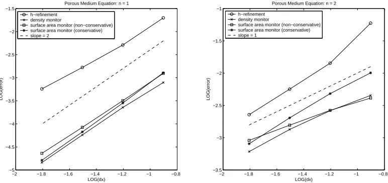
−2 −1.8 −1.6 −1.4 −1.2 −1 −0.8 −5 −4.5 −4 −3.5 −3 −2.5 −2 −1.5 LOG(dx) LOG(error)

Porous Medium Equation: n = 1

h−refinement density monitor

surface area monitor (non−conservative) surface area monitor (conservative) slope = 2

−2 −1.8 −1.6 −1.4 −1.2 −1 −0.8 −3.5 −3 −2.5 −2 −1.5 −1 LOG(dx) LOG(error)

Porous Medium Equation: n = 2

h−refinement density monitor

surface area monitor (non−conservative) surface area monitor (conservative) slope = 1

Fig. 1. Comparison ofL1 errors for the different approximation schemes.

Figures 1 and 2 show how theL1 _{and L}2 _{errors vary with the size of the mesh}

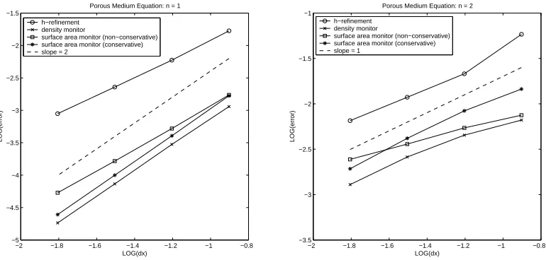
−2 −1.8 −1.6 −1.4 −1.2 −1 −0.8 −5

−4.5 −4 −3.5 −3 −2.5 −2 −1.5

LOG(dx)

LOG(error)

Porous Medium Equation: n = 1

h−refinement density monitor

surface area monitor (non−conservative) surface area monitor (conservative) slope = 2

−2 −1.8 −1.6 −1.4 −1.2 −1 −0.8 −3.5

−3 −2.5 −2 −1.5 −1

LOG(dx)

LOG(error)

Porous Medium Equation: n = 2

h−refinement density monitor

surface area monitor (non−conservative) surface area monitor (conservative) slope = 1

Fig. 2. Comparison ofL2 errors for the different approximation schemes.

more time steps). The h-refinement method has been used in a manner which covers the support of the solution with a uniform quadrilateral mesh of size

dx. Both sets of results were initialised using (52) with r0 = 1.0 and t = t0, where t0 is the initial time calculated using (53), and the comparisons are made at T = 0.04 where T =t−t0.

Typically the density monitor m=u gives the most accurate approximations at these mesh resolutions, but the surface area monitor with conservative ALE recovery for u appears to exhibit a slightly higher order of accuracy, partic-ularly when n = 2. In general the moving mesh method loses an order of accuracy when n = 2, where the gradient of the exact solution is infinite at the boundary. The apparent lower accuracy of the h-refinement approach in this case is not surprising because the solutions it is approximating have in-finite second derivative at the moving boundary which is, in this case, inside the domain. It is also worth noting that for both n = 1 and n = 2 mass conservation is important for maintaining accuracy. In [6] the problem of re-duced accuracy at the front is successfully treated in one dimension using h

refinement within the moving frame.

10.2 Numerical results for non-self-similar solutions

The benchmark adaptive h-refinement scheme that is used is based upon a standard quad-tree data structure for the organisation of a hierarchical mesh of bilinear quadrilateral elements. This mesh may be refined to different levels in different geometric regions with the restriction that no neighbouring ele-ments may be more than one level apart in the hierarchy. This ensures that no elements in the mesh have any edges with more than one “hanging node”. The solution procedure on this mesh is based upon a standard finite element discretisation of the PME on a spatial domain that far exceeds the support of the initial data. This leads to an ordinary differential equation (ODE) sys-tem for the nodal solution values which is solved using an implicit, second order scheme (the trapezoidal rule). At each time-step this requires the solu-tion of a system of nonlinear algebraic equasolu-tions which is found using a full approximation scheme (FAS) multigrid algorithm, as described in [12]. This particular solver deals with the hanging nodes quite naturally by prescribing the solution values at such points to be the average of the values at the ends of the edge upon which the hanging node lies, [14]. Furthermore, because the implicit time-stepping scheme is a one-step method it is straightforward to adapt the mesh at the end of each step and interpolate the latest solution onto the new mesh before continuing.

For the purposes of the benchmark solutions obtained here a particularly cau-tious adaptivity strategy is used (relative efficiency not being an issue consid-ered here). This essentially undertakes uniform refinement up to a maximum prescribed level wherever the solution is non-zero (to be more precise, |u| ≤ε

for some small choice of ε). In addition, numerous “safety layers” of refine-ment are imposed around the edge of this refined region and further safety layers of elements are imposed at each level of the mesh hierarchy down to the coarsest mesh. A typical mesh, with a maximum refinement level of 8, is shown in Figure 3 (right). It should be noted that, in all of the examples shown, the spatial error dominates the temporal error (reducing the length of the time-steps has little effect on the overall error) and the solutions are not affected significantly by altering either the value of ε or the number of safety layers in the adaptive algorithm. In the comparisons that follow the level 9 mesh is used (the finest of the ones for which results are presented in Section 10.1).

The first set of problems studied in this section are radially symmetric and use the initial conditions (when t=t0) of the self-similar solutions (52),

u(r, t0) =

"

max

Ã

1− µr

r0

¶2

,0

!#_n1

(54)

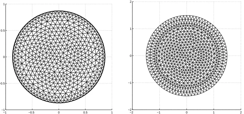
self-Fig. 3. The initial, 615 node, 1149 cell, unstructured triangular mesh used for all of the radially symmetric, non-self-similar, moving mesh results withr0 = 0.5 (left) and a typical initial adaptive quadrilateral mesh (shown to level 8 meshes) as constructed by the h-refinement approach on the much larger domain [−4,4]×[−4,4] (right).

similar solution for n = 1 the solution is evolved according to the PME with

n = 2, and vice versa. In all cases the moving mesh method uses the scale-invariant forward Euler time-stepping with constant dσ = 0.0001. The initial mesh used to produce all the moving mesh results is shown in Figure 3 (left), along with a typical initial mesh used by the h-refinement approach (right, and shown on a different scale since this initial mesh covers a much larger region).

−1 −0.5 0 0.5 1 0

0.25 0.5 0.75 1

Porous Medium Equation: n = 2

x

u

−1.5 −1 −0.5 0 0.5 1 1.5 0

0.25 0.5 0.75 1

Porous Medium Equation: n = 1

x

u

−1 −0.5 0 0.5 1

0 0.25 0.5 0.75 1

Porous Medium Equation: n = 2

x

u

−1.5 −1 −0.5 0 0.5 1 1.5 0

0.25 0.5 0.75 1

Porous Medium Equation: n = 1

x

u

−1 −0.5 0 0.5 1

0 0.25 0.5 0.75 1

Porous Medium Equation: n = 2

x

u

−1.5 −1 −0.5 0 0.5 1 1.5 0

0.25 0.5 0.75 1

Porous Medium Equation: n = 1

x

u

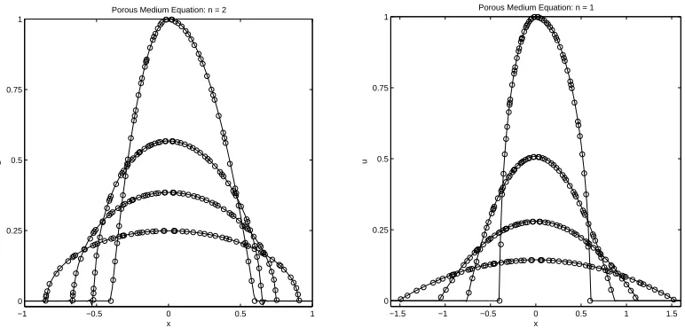
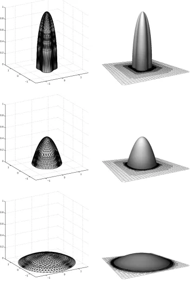
Fig. 4. Slices through the solution surface alongy = 0 comparing the h-refinement method (solid lines) with three moving mesh methods (circles): ˜m=uwith direct re-covery of the solution (top) and ˜m=t−dβp

gradients in the direction where the element is shortest) [1,13]. −1 −0.5 0 0.5 1 −1 −0.5 0 0.5 1 0 0.2 0.4 0.6 0.8 1 −1 −0.5 0 0.5 1 −1 −0.5 0 0.5 1 0 0.2 0.4 0.6 0.8 1

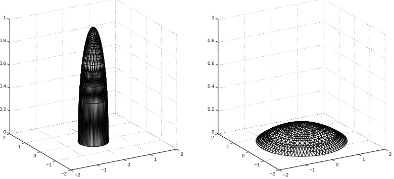
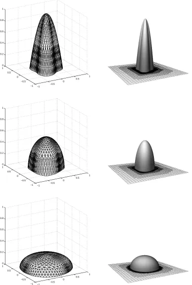
Fig. 5. The initial (left) and final (right) solution surfaces obtained using the moving mesh method with the surface area type monitor and conservative ALE recovery, with initial conditions calculated from the self-similar solution usingn= 1 and the evolution governed by the PME withn= 2.

−2 −1 0 1 2 −2 −1 0 1 2 0 0.2 0.4 0.6 0.8 1 −2 −1 0 1 2 −2 −1 0 1 2 0 0.2 0.4 0.6 0.8 1

Fig. 6. The initial (left) and final (right) solution surfaces obtained using the moving mesh method with the surface area type monitor and conservative ALE recovery, with initial conditions calculated from the self-similar solution with n= 2 and the evolution governed by the PME withn= 1.

It is informative here to consider the evolution of the integrals on the left-hand side of (19) after U has been recovered. Figure 8 contains plots of the value of this quantity associated with 15 representative mesh nodes (those closest to a ray emanating from the centre of the domain along the negative

−1 −0.5 0 0.5 1 −1

−0.5 0 0.5 1

−2 −1 0 1 2

−2 −1 0 1 2

Fig. 7. The final meshes obtained using the moving mesh method with the surface area type monitor and conservative ALE recovery, with initial conditions calculated from the self-similar solution with n= 1 and the evolution governed by the PME withn= 2 (left) and vice versa (right).

with which the mesh velocity is calculated and constrained by total mass conservation. The initial perturbations are far more pronounced in the non-self-similar case, where these integrals are not expected to remain exactly constant after recovery, particularly at the nodes near to the boundary where the additional recovery stages also have some effect on the accuracy of the approximation. Subsequently, the local integrals in both cases become almost constant. The integral of the monitor over the whole domain exhibits similar behaviour: in the non-self-similar case it drops by about 10% in the early stages and then settles down: in the self-similar case it varies by less than 1%.

Finally, the fixed and moving mesh approaches are compared for problems which do not possess any radial symmetry. The initial conditions are now given by

u(r, t0) =



max 

1− Ã

r r′

0

!2

,0



 



1

n

(55)

where

r′

0 = r0(1 +ǫcos(Ntan−1(y/x))).

0 1 2 3 4 5 0

0.002 0.004 0.006 0.008 0.01 0.012

Porous Medium Equation: n=1

Time

Local integral

0 1 2 3 4 5

0 2 4 6 8x 10

−3 _{Porous Medium Equation: n=2}

Time

Local integral

Fig. 8. The evolution of the values of the local integral of the scale-invariant monitor associated with 15 representative mesh nodes, using the surface area monitor and conservative ALE recovery, with initial conditions given by the self-similar solution with n = 1 and the evolution governed by the PME with n = 1 (left) and n = 2 (right).

mesh shown in Figure 3 (left) undergoes the transformation

xi = xi(1 +ǫcos(Ntan−1(y/x))).

In this case only the surface area monitor (which moves points towards regions where the solution gradient increases) is used, combined with conservative ALE recovery (which has shown itself to be superior to the non-conservative approach), for the comparison.

The solutions can still be compared adequately using slices through the data alongy= 0 and these are shown in Figure 9. It is clear that the two approaches again agree closely for these cases. The evolution of the solution surfaces for the two methods are compared in Figures 10 and 11, which illustrate that no anomalies were hidden by only taking slices through the data. The initial and final meshes for the moving mesh approach are shown for both cases in Figures 12 and 13 and exhibit similar qualitative features to the earlier results.

11 Discussion

−1 −0.5 0 0.5 1 0

0.25 0.5 0.75 1

Porous Medium Equation: n = 2

x

u

−1.5 −1 −0.5 0 0.5 1 1.5 0

0.25 0.5 0.75 1

Porous Medium Equation: n = 1

x

u

Fig. 9. Slices through the solution alongy = 0 comparing the moving mesh method (circles) with theh-refinement approach (solid lines). Initial conditions are derived from (55) withn= 1 and the evolution governed by the PME withn= 2 (left) or vice versa (right). The four snapshots are taken atT = 0.0,0.125,0.5,2.0.

of which, based on surface area, is illustrated in this paper) used to drive the mesh movement through a conservation principle, and the use of scale-invariant time-stepping which yields a scheme with uniform local truncation error in time.

Results have been presented for a variety of test cases using the porous medium equation in two space dimensions and have been validated against self-similar analytical solutions and other solutions. In the latter case they have been com-pared with results from a state-of-the-arth-refinement finite element approach on uniform quadrilateral meshes. It has been shown that the conservative ALE approach provides the best means of recovering solution values at the nodes once the mesh velocity has been obtained and that the resulting scale-invariant moving mesh method is highly accurate. This remains true even in cases when the conservation principle (19) is only approximately constant in time (i.e.

non-self-similar solutions simulated using the surface area monitor), so long as the monitor is only used in the construction of the mesh velocities, not the recovery of the dependent variable, and so long as the scale-invariant version of the monitor is used. (Note that results obtained using the unscaled monitor are extremely poor.)

−1

−0.5 0 0.5

1

−1 −0.5 0 0.5 1 0 0.2 0.4 0.6 0.8 1

−1 −0.5 0

0.5 1

−1 −0.5 0 0.5 1 0 0.2 0.4 0.6 0.8 1

−1 −0.5 0

0.5 1

−1 −0.5 0 0.5 1 0 0.2 0.4 0.6 0.8 1

−1 0

1 −1

0 1 0 0.2 0.4 0.6 0.8 1

−1 0

1 −1

0 1 0 0.2 0.4 0.6 0.8 1

−1 0

1 −1

0 1 0 0.2 0.4 0.6 0.8 1

−1 −0.5 0 0.5 1 −1

−0.5 0 0.5 1

−1 −0.5 0 0.5 1

−1 −0.5 0 0.5 1

Fig. 12. The initial (left) and final (right) meshes obtained using the moving mesh method with non-radially-symmetric initial conditions calculated using (55) with n= 1 and the evolution governed by the PME with n= 2.

−1 0 1

−1 0 1

−1 0 1

−1 0 1

Fig. 13. The initial (left) and final (right) meshes obtained using the moving mesh method with non-radially-symmetric initial conditions calculated using (55) with n= 2 and the evolution governed by the PME with n= 1.

approach with fewer degrees of freedom.

References

[1] Apel T, Grosman S, Jimack PK, Meyer A. A new methodology for anisotropic mesh refinement based upon error gradients. Appl. Numer. Math. 2004; 50_:

329-341.

[3] Baines MJ, Hubbard ME, Jimack PK. A moving mesh finite element algorithm for the adaptive solution of time-dependent partial differential equations with moving boundaries.Appl. Numer. Math. 2004; to appear.

[4] Barenblatt GI.Scale Invariance, Self-similarity and Intermediate Asymptotics.

CUP 1996.

[5] Beckett G, Mackenzie JA, Robertson ML. A moving mesh finite element method for the solution of two-dimensional Stefan problems. J. Comput. Phys. 2001;

168_:500–518.

[6] Blake KW, Baines MJ. A moving mesh method for nonlinear parabolic problems. Numerical Analysis Report 2/2002, Department of Mathematics, University of Reading, 2002.

[7] Blake KW.Moving Mesh Methods for Nonlinear Partial Differential Equations. PhD Thesis, University of Reading, 2001. (See also Blake KW, Baines MJ, Numerical Analysis Report 2/02, Department of Mathematics, University of Reading, UK.)

[8] Budd CJ, Leimkuhler B, Piggott M. Scaling invariance and adaptivity. Appl. Numer. Math.2001;39_{: 261-288.}

[9] Budd CJ, Piggott M. Geometric integration and its applications. Handbook of Numerical Analysis, XI 2003; 128_:35–139.

[10] Cao W, Huang W, Russell RD. A moving mesh method based on the geometric conservation law.SIAM J. Sci. Comput. 2002; 24_:118–142.

[11] Huang W, Ren Y, Russell RD. Moving mesh partial differential equations (MMPDEs) based on the equidistribution principle. SIAM J. Numer. Anal.

1994; 31_:709–730.

[12] Jones AC, Jimack PK. An adaptive multigrid tool for elliptic and parabolic systems Int. J. Numer. Meth. Fluids 2004; to appear.

[13] Kunert, G. Robust local problem error estimation for a singularly perturbed problem on anisotropic finite element meshes.Math. Model. Numer. Anal.2001;

35_{:1079–1109.}

[14] Meyer A. Projection techniques embedded in the PCGM for handling hanging nodes and boundary restrictions. In Engineering Computational Technology,

Topping B.H.V, Bittnar Z (eds). Saxe-Coburg Publications, Stirling, Scotland, 2002; 147–165.

[15] Miller K, Miller RN. Moving finite elements, part I. SIAM J. Numer. Anal.

1982; 18_{:1019–1057.}

[16] Murray JD. Mathematical Biology: An Introduction (3rd edition). Springer, 2002.