Reducing computational effort in field optimisation problems

Reducing computational effort

in ®eld optimisation problems

J.K. Sykulski

Department of Electronics and Computer Science, University of Southampton, Southampton, UK

Keywords Finite element analysis, Electromagnetism, Optimization techniques

AbstractDesign and optimisation of many practical electromechanical devices involve intensive ®eld simulation studies and repetitive usage of time-consuming software such as ®nite elements (FEs), ®nite differences of boundary elements. This is a costly, but unavoidable process and thus a lot of research is currently directed towards ®nding ways by which the number of necessary function calls could be reduced. New algorithms are being proposed based either on stochastic or deterministic techniques where a compromise is achieved between accuracy and speed of computation. Four different approaches appear to be particularly promising and are summarised in this review paper. The ®rst uses a deterministic algorithm, known as minimal function calls approach, introduces online learning and dynamic weighting. The second technique introduced as ES/DE/MQ – as it combines evolution strategy, differential evolution and multiquadrics interpolation–offers all the advantages of a stochastic method, but with much reduced number of function calls. The third recent method uses neuro-fuzzy modelling and leads to even further economy of computation, although with slightly reduced accuracy of computation. Finally, a combined FE/neural network approach offers a novel approach to optimisation if a conventional magnetic circuit model could also be used.

1. Introduction

Optimal design of electromechanical devices often necessitates repetitive usage of ®nite element (FE) solvers or other numerically intensive ®eld computation. A direct way of incorporating ®eld modelling into an optimisation loop is to call the FE package every time a function evaluation is needed. Although fairly straightforward in implementation, this online approach will normally lead to unacceptable computing times, as for each set of selected design parameters a full ®eld analysis needs to be undertaken. The number of necessary calls to the FE software escalates as the number of design variables increases; moreover, additional calls are normally required to calculate each gradient of the objective function. Although theoretically this is of no consequence, in the design of®ce environment such an approach becomes impractical.

2. Minimal function calls approach

The minimum function calls (MFCs) approach relies on evaluating the objective function a priori for a number of pre-determined cases and ®tting an interpolating function through the data points (Al-Khoury and Sykulski, 1998; Sykulski and Al-Khoury, 2000; Sykulskiet al., 2001). The optimiser then uses the interpolating function rather than calling the FE directly. In this response surface methodology (RSM) (Pahner and Hameyer, 1999) it is usual to use

The Emerald Research Register for this journal is available at The current issue and full text archive of this journal is available at www.emeraldinsight.com/researchregister www.emeraldinsight.com/0332-1649.htm

Reducing

computational

effort

159

COMPEL: The International Journal for Computation and Mathematics in Electrical and Electronic Engineering Vol. 23 No. 1, 2004 pp. 159-172

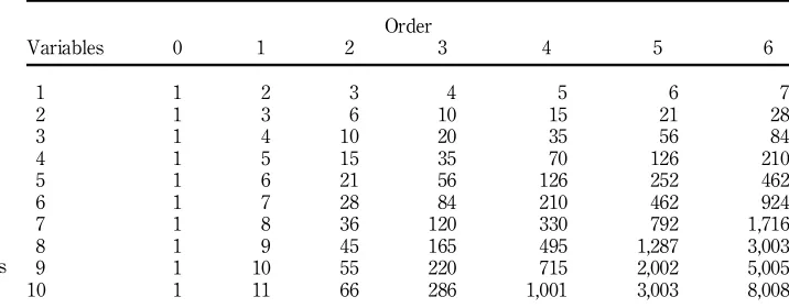
polynomial interpolating functions. Table I shows the number of coef®cients in the interpolating equation for various number of variables and orders of polynomials ®t. As an illustration, the second-order two variables case requires six coef®cients c1x21+ c2x1x2+ c3x22+ c4x1+c5x2+ c6. The ®t order de®nes the maximum total order of any one polynomial term. For example, for third-order, x3

1 and x32 are used, but not x21x22. It should be noted that the minimum number of function evaluations needed for curve ®tting is equal to the number of coef®cients in the interpolating equation. For each point used in the curve ®tting, a full FE simulation is required. The number of such calls is much less than if the FE simulation function was to be called directly by the optimiser. For example, using a third-order polynomial and ®ve design variables requires 56 function calls, which will be quite acceptable in practical situations.

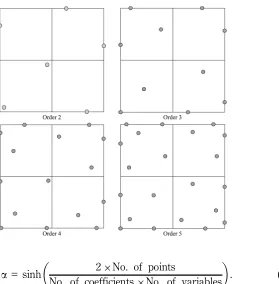
In the MFC approach, the position of initial points is carefully selected to be optimal in a sense that the resulting algorithms have proven stable (Sykulski

et al., 2001). As an example, Figure 1 shows the distribution of initial points for two variables with different orders of polynomial ®t. It can be seen that points ®ll the search space and do not form regular arrays.

Using RSM, the computing times reduce dramatically, but care must be taken not to sacri®ce accuracy. Extensive numerical experiments have shown that further signi®cant improvements may be achieved by introducingonline learningwithdynamic weighting(Sykulskiet al., 2001).

As the optimisation process proceeds, more points become available for curve ®tting and thus, the estimate of the optimum position becomes more accurate. It is therefore appropriate to apply lower weighting to points far from the predicted optimum. The weighting factor for each point is given by

Weighting factor = exp(_a(x2 xRef)2), (1)

wherexis the input vector for each point andx_Refis the input vector for the best point for which a FE solution is available. The value of_ais given by

Order

Variables 0 1 2 3 4 5 6

1 1 2 3 4 5 6 7

2 1 3 6 10 15 21 28

3 1 4 10 20 35 56 84

4 1 5 15 35 70 126 210

5 1 6 21 56 126 252 462

6 1 7 28 84 210 462 924

7 1 8 36 120 330 792 1,716

8 1 9 45 165 495 1,287 3,003

9 1 10 55 220 715 2,002 5,005

10 1 11 66 286 1,001 3,003 8,008

Table I.

The number of necessary function calls for RSM

COMPEL

23,1

a = sinh 2£No. of points

No. of coefficients_£No. of variables

³ ´

. (2)

The hyperbolic sine function is chosen because initially, all points are equally weighted, while for large number of points, the radius of the Gaussian function reduces exponentially. The rate of this exponential reduction is chosen, so that as each new point is added, approximately (on average) one point will move outside the radius. At the same time,learning pointsare added, which are not placed at the predicted optimum and thus allow the modelling of the normal gradients of the objective and constraint functions to be re®ned.

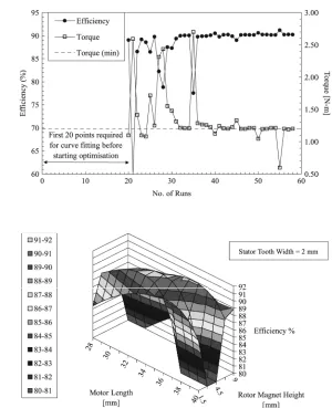
To illustrate the process, a brushless permanent magnet motor has been optimised for ef®ciency (with minimum torque constraint) in terms of magnet height, tooth width and stack length. The convergence is shown in Figure 2. It should be noted that, since every ®fth point is a learning point, these points are not placed at the predicted optimum. Figure 3 shows a section through the response surface illustrating the nature of the optimisation problem. The ef®ciency is calculated by integrating input power and losses in a time-stepping model.

3. Evolution strategies

The deterministic approach of Section 2, despite the addition of learning points, may not be able to avoid local minima traps. If this is identi®ed as a potential

Figure 1.

Optimal positions of initial points for the case of two variables and different order of interpolating polynomial function

Reducing

computational

effort

problem, then stochastic techniques may offer a better choice. Most such techniques are very expensive in terms of number of necessary function evaluations and thus, impractical. Some more recent methods, however, look more promising and one such technique introduced originally in the work Farina and Sykulski (2001) is reported here. It uses a combination of evolution strategy, differential evolution and multiquadrics interpolation (ES/DE/MQ) as shown in Figure 4.

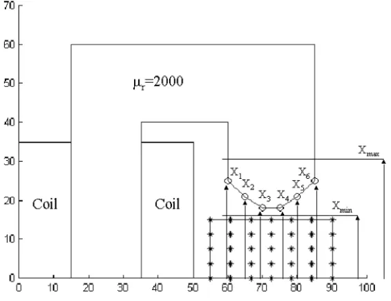
Consider a C-core where the pole faces are to be shaped to achieve homogeneous magnetic ®eld in a rectangular region in the centre of the air gap. The ®eld at 35 points on a regular grid is evaluated and the objective function is computed

Figure 2.

Convergence of ef®ciency and torque

Figure 3.

Brushless PM motor optimisation response surface

COMPEL

23,1

FC =

imax= 1,35jB02 Bij(B0)

2 1_{, (3)}

whereBiare magnetic ®eld values on the grid andB0is the value at the centre.

The design variables are the coordinates of the six points (x1-x6) de®ning the

shape of the pole face. The geometry, design constraints and the control grid are shown in Figure 5.

Figure 4.

Flowchart of the

ES/DE/MQmethod (Farina and Sykulski, 2001)

Figure 5.

The geometry of the C-core shaped magnet

Reducing

computational

effort

The results of the optimisation are compared with optimum con®gurations obtained with standard techniques on the real objective function (full direct search). Three standard strategies (one ES and two versions of DE1 and DE2) and a gradient based algorithm (GBA) have been considered. The latter is the MatlabFMINCONoptimisation function.

As shown in the last column in Table II the number of objective function calls is greatly reduced (it is even notably smaller than for the direct method GBA), whereas the value of the objective function is similar to ES and DE2 results and better than those obtained with DE1 and GBA. The optimal con®guration is shown in Figure 6.

This hybridES/DE/MQ method has been shown to be able to avoid local minima traps for a number of test functions and achieves a signi®cant reduction in the number of necessary function calls, making the approach suitable for computationally intensive FE design/optimisation problems. Moreover, the quality of the resultant optimum is comparable to, or better than, those obtained using other methods.

4. Neuro-fuzzy modelling

This recent technique employs the neuro-fuzzy modelling (NFM) (Rashidet al., 2001b) and uses optimisation based on the genetic algorithm (GA) and the sequential quadratic programming (SQP) method (Rashid et al., 2000a, b, 2001a). In the NF/GA/SQP approach, ann-dimensional hyper-space is sampled initially using a grid structure or a suitable design of experiment (DoE)

Starting Optimum n

DE1 9 random 0.0803 720

DE2 13 random 0.0704 881

ES 0.7532/0.4344/0.6411 0.0642 450

GBA 0.7532 0.0855 188

ES/DE/MQ 0.7532 0.0718 118

Table II.

Comparative optimisation results for a C-core

Figure 6.

C-core optimal con®guration

COMPEL

23,1

orthogonal array (Fowlkes and Creveling, 1995) if the number of variables is high. The model data is subsequently employed to create a neuro-fuzzy model, which provides an approximation of real function. The notion of membership functions (MFs) is introduced which can be described by Gaussian, generalised bell or other curves. During the supervised training process, the parameters of each MF are modi®ed using the back-propagation algorithm and the consequent parameters are established using least squares, ultimately providing an approximation of the system under investigation. This empirical model then effectively replaces the actual function generator, in this case the FE solver, easing the computational cost when applying the optimisation routine. This comprises a GA to identify the locality of the global optimum followed by the SQP method to isolate it accurately. The latter is possible due to the extraction of derivative information from the neuro-fuzzy model.

In order to minimise the cost of sampling, the hyper-surface is iteratively re®ned by addition of the perceived optimum, a number of genetically sampled points and a number of random samples for explorative purposes to the model data-set. The grid is also reset after a number of iterations to concentrate on the area of interest. The process is repeated until the stopping criterion is met. That is, when convergence to an optimal point occurs, given by the in®nity norm between the successive perceived optimum points or on reaching the maximum number of iterations or sample points (Rashidet al., 2001b).

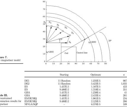
Consider a magnetiser problem with six design parameters (Gallardo and Lowther, 1999; Mohammed and Uler, 1997), as shown in Figure 7. The design objective is to model the pole face, using the six free nodes, to realize a sinusoidal ®eld along the chordAB. Results are obtained for the unconstrained problem in which all node vectors are assumed feasible and the constrained case in which certain vectors are assumed infeasible to avoid non-smooth designs. In practice, this means that the gradients of each of the ®ve chords in Figure 7 must remain negative. Thus, additional constraints, other than those pertaining to the problem bounds, are imposed (Rashidet al., 2001b), and poor regions of design space are discarded.

The basic objective function is given by:

f = X 59

k= 1

(Bdesired,k2 Bcalculated,k)2 (4)

where

Bdesired,k = Bmaxsin(908 2 k)

with 1# k# 59.

The results for unconstrained optimisation are summarised in Table III and compared with the ES/DE/MQ method of Section 3, as well as with standard

Reducing

computational

effort

evolutionary strategies and MATLAB’s GBA (similar comparison to that of Table II). In the NF/GA/SQP approach, the initial design space is sampled using an orthogonal experimental design array yielding 27 samples (Uler and Mohammed, 1996), complemented with 23 randomly selected samples to give an initial data-set of 50 points. Sampling in subsequent iterations is composed of the pseudo optimum, a number of genetic samples and a number of random samples. In the ES/DE/MQ approach, a pseudo-grid using an initial node set of 64 points (2ndof) is employed, where each of the six points Pi assumes two possible values given by the range limits or constraints. Results from constrained optimisation are described in Table IV.

It is very satisfying to see that both methods achieve good results with signi®cant reduction in the number of function calls compared with more

Starting Optimum n

DE1 11 Random 1.235E-5 987

DE2 11 Random 5.423E-5 1,035

ES 1.457E-3 1.187E-5 433

ES 9.486E-2 1.318E-4 351

GBA 1.457E-3 1.238E-4 41

GBA 9.486E-2 2.433E-4 281

ES/DE/MQ 1.457E-3 1.961E-5 234

ES/DE/MQ 9.486E-2 2.125E-5 206

NF/GA/SQP – 6.570E-5 189

Table III.

Unconstrained optimisation results for magnetiser

Figure 7.

The magnetiser model

COMPEL

23,1

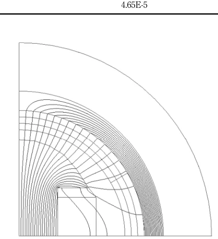
standard methods. The introduction of constraints seems to be particularly effective for NF/GS/SQP approach, improving the pro®le of the pole face and taking signi®cantly fewer samples as expected. The DE/ES/MQ algorithm gives slightly better results in both cases, but requires more samples, surprisingly even more in the constrained case. The optimal shape obtained with the unconstrained ES/DE/MQ method is shown in Figure 8.

The success of both the methods lies in their ability to search unexplored regions of space whilst exploiting available knowledge to identify more accurately regions of minima. On an average the DE/ES/MQ method ®nds a slightly better solution at the cost of a greater number of function evaluations. Both methods, however, require the number of function calls much lower than would be expected using conventional stochastic methods (Gallardo and Lowther, 1999; Mohammed and Uler, 1997; Uler and Mohammed, 1996), and this is where the bene®ts of such approaches lie, in improving the ef®ciency of the optimisation process whilst maintaining solution accuracy.

5. Combined FEs/neural networks

There is growing interest in the ways in which the performance of a speci®c device could be modelled using a neural network. Such a network learns the

Figure 8.

Magnetiser optimal con®guration obtained from ES/DE/MQ (Farina and Sykulski, 2001)

Optimum n

ES/DE/MQ 1.58E-5 246

NF/GA/SQP 4.65E-5 155

Table IV.

Constrained optimisation results for magnetiser

Reducing

computational

effort

shape of the hyper-surface and provides a fast evaluation of any point in it. Typically, the neural network is trained in a batch mode, prior to the optimisation process – essentially ªoff-lineº (Arkadan and Chen, 1994; Ratner

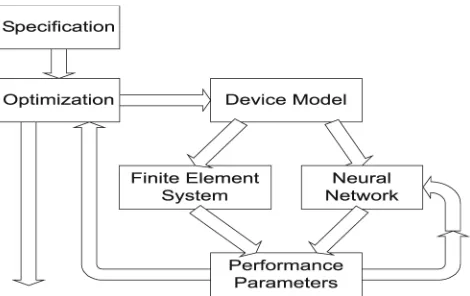
et al., 1996). A recent attempt has been made to construct a system which can provide ªonlineº training, i.e. a network which is capable of learning and modifying its behaviour as it is used (Seguinet al., 1999). Such a network has major bene®ts over a static system in that it can handle a large number of variations of a device and track developments in design related to material changes and manufacturing processes. A diagram of the system is shown in Figure 9. This differs from a conventional system in that the numerical analysis (FE) component and the neural network exist in parallel and data can ¯ow either way from the device model to determine the performance parameters. Each time, a set of performance parameters is generated, the data are fed back to provide a new training set for the neural network. Initially, as in the earlier proposed systems, the network is trained off-line on a device typical of the class of problems to be handled. The decision on which approach to take to generate the performance parameters is made within the device model by an intelligent system which contains a description of the current capabilities of the neural network and relates these to the problem being considered.

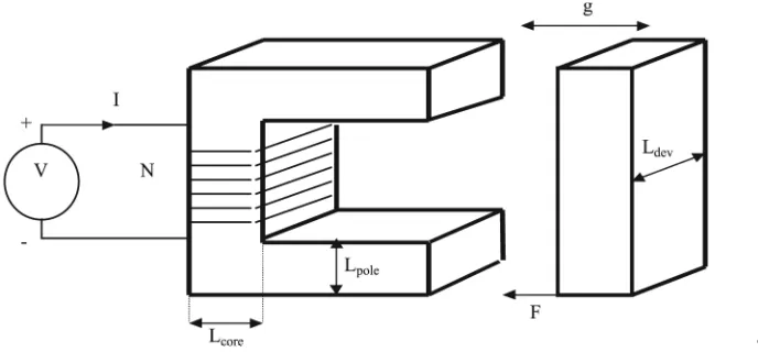
The neural network component of the architecture shown in Figure 9 consists of two parts. The ®rst is intended to produce the actual values of the parameters for the speci®ed device in a manner similar to that described by Arkadan and Chen (1994) and Ratneret al.(1996); the second part indicates the sensitivity of the device to changes in the inputs. This latter information is then used to guide the optimiser. The sensitivity prediction part of the system is described by Seguinet al.(1999) and is based on a knowledge-based network (Dandurand and Lowther, 1999), which implements a set of simple rules derived from a magnetic circuit. This is then corrected by the addition of an error prediction network trained on numerical examples. An example of a simple C-core actuator has been used (Figure 10).

Figure 9.

Design process using online neural network

COMPEL

23,1

First, a conventional magnetic circuit model of the device is developed to create a set of sensitivity rules which guide the optimisation. Such a model is necessarily simpli®ed and the effects of non-linearity and leakage ultimately need to be included. These may be considered as local perturbations on the underlying magnetic circuit structure. Thus, an ef®cient route to achieve a fast and accurate prediction of the device performance is to measure the error between the magnetic circuit prediction and the numerical analysis. This error can be determined online and can be learnt by a second neural network operating in concert with the knowledge-based system. In order to achieve this, theerror correcting network needs to have the capability to correct the error ªlocallyº within the design space and aradial basis functionnetwork has been found to be well suited to perform this task. A series of tests were performed with the objective to minimise the error as the device was driven into saturation and the fringing and non-linearity effects became more important. In this sense, the neural network system can take over from a full numerical (FE) analysis once it has been trained thus, providing either a designer or an optimisation system with extremely fast turnaround times on design modi®cations.

6. Pareto optimisation

The design of electromechanical devices has to be put in the context of general trends and developments of optimisation methods (Neittaanmakiet al., 1996; Russenschuck, 1996). The role of multi-objective optimisation (Deb, 2001; Schatzeret al., 2000; Thiele and Zitzler, 1999) is increasing as practical designs usually involve con¯icting requirements. Traditionally, such problems are often converted into single-objective tasks with a priori application of some knowledge or imposition of a decision (for example, throughweighting factors), but it is argued that information can easily be lost in the process and some existing ªoptimalº solutions may even be mathematically impossible to achieve. Instead the application of pareto optimal front (POF) approximation is

Figure 10.

A simple C-core actuator (Seguinet al., 1999)

Reducing

computational

effort

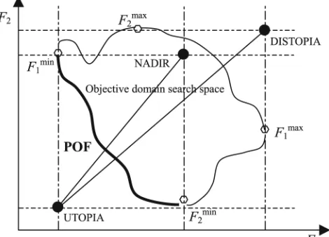
advocated. The mathematical theory of Pareto multi-objective optimisation may be somewhat complicated (Deb, 2001, Miettinen, 1999) but some basic de®nitions and properties are easily explained using a special case of two objective functions being minimised as shown in Figure 11.

A multi-objective problem may be convex or non-convex, discontinuous,

deceptiveormultimodal, and there are various ways of treating such conditions. The important point is that a result is not a single solution, but a set of possible (and in some sense acceptable) solutions given by various combinations of design parameters (the design domain search space is not shown here, but could consist of a number of variables). The ®nal decision about the choice of the design is therefore made a posteriori and any point on the POF may be considered optimal. Such information is clearly more helpful to a designer than a result from a single-objective model.

A comprehensive treatment of POF approximations for multi-objective shape design optimisation may be found in the work of Farina (2002), including several practical examples (air-cored solenoid, electrostatic micromotor, single-phase reactor and inductor for transverse ¯ux heating).

7. Conclusions

In this paper, it has been argued that optimisation methods have achieved a status of a mature tool which can be applied ef®ciently to practical design problems requiring accurate, but time-consuming, ®eld simulations. There are a vast number of methods and techniques of optimisation and the dif®culty is that the choice of the ªbestº one is problem dependent. In this paper, attention has been drawn on methods particularly suitable to computationally intensive design problems, such as those which arise when a FE (or similar) method has to be used for accurate prediction of performance. Most of such methods are

Figure 11.

Example of objective domain search space showing the POF and UTOPIA, DISTOPIA and NADIR points

COMPEL

23,1

based on RSM. If local minima traps are considered not to be a problem, a deterministic method such as MFCs approach is recommended. Particular combinations of evolutionary strategies and GAs have also been designed and reported here for increasing the chances of ®nding the global optimum. Some recent work on application of neural networks also looks promising. Finally, the importance of multi-objective optimisation has been stressed.

References

Al-Khoury, A.H. and Sykulski, J.K. (1998), ªAutomation of ®nite element aided design of brushless PM motorsº,Proceedings of ICEM’98, 2-4 September 1998, Istanbul, Turkey, pp. 614-8.

Arkadan, A.A. and Chen, Y. (1994), ªArti®cial neural network for the inverse electromagnetic problem of system identi®cationº,Southeastcon ’94, April 1994, Miami, USA, pp. 162-4. Dandurand, F. and Lowther, D.A. (1999), ªElectromagnetic device performance identi®cation

using knowledge based neural networksº,IEEE Transactions on Magnetics, Vol. 35 No. 3, pp. 1817-20.

Deb, K. (2001),Multi-objective Optimization Using Evolutionary Algorithms, Wiley, Chichester. Farina, M. (2002), ªCost-effective evolutionary strategies for Pareto optimal front approximation

to multi-objective shape design optimization of electromagnetic devicesº, PhD dissertation, Department of Electrical Engineering, University of Pavia, Italy.

Farina, M. and Sykulski, J.K. (2001), ªComparative study of evolution strategies combined with approximation techniques for practical electromagnetic optimisation problemsº, IEEE Transactions on Magnetics, Vol. 37 No. 5, pp. 3216-20.

Fowlkes, W.Y. and Creveling, C.M. (1995),Engineering Methods for Robust Product Design, Addison-Wesley, New York.

Gallardo, J.A. and Lowther, D.A. (1999), ªThe optimisation of electromagnetic devices using niching genetic algorithmsº,COMPEL, Vol. 18 No. 3, pp. 285-97.

Miettinen, K. (1999),Nonlinear Multiobjective Optimisation, Kluwer, Dordrecht, The Netherlands. Mohammed, O.A. and Uler, F.G. (1997), ªA hybrid technique for the optimal design of electromagnetic devices using direct search and genetic algorithmsº,IEEE Transactions on Magnetics, Vol. 33 No. 2, pp. 1931-4.

Neittaanmaki, P., Rudnicki, M. and Savini, A. (1996),Inverse Problems and Optimal Design in Electricity and Magnetism, Oxford Science Publications, Oxford.

Pahner, U. and Hameyer, K. (1999), ªAdaptive coupling of differential evolution and multiquadrics approximation for the tuning of the optimization processº,Proceedings of COMPUMAG Sapporo, 25-28 October 1999, pp. 116-7.

Rashid, K., Ramirez, J.A. and Freeman, E.M. (2000a), ªHybrid optimisation in electromagnetics using sensitivity information from a neuro-fuzzy modelº, IEEE Transactions on Magnetics, Vol. 36 No. 4, pp. 1061-5.

Rashid, K., Ramirez, J.A. and Freeman, E.M. (2000b), ªA general approach for extracting sensitivity analysis from a neuro-fuzzy modelº,IEEE Transactions on Magnetics, Vol. 36 No. 4, pp. 1066-70.

Rashid, K., Ramirez, J.A. and Freeman, E.M. (2001a), ªOptimisation of electromagnetics devices using sensitivity information from clustered neuro-fuzzy modelsº,IEEE Transactions on Magnetics, Vol. 37 No. 5, pp. 3575-8.

Reducing

computational

effort

Rashid, K., Farina, M., Ramirez, J.A., Sykulski, J.K. and Freeman, E.M. (2001b), ªA comparison of two generalized response surface methods for optimisation in electromagneticsº,

COMPEL, Vol. 20 No. 3, pp. 740-52.

Ratner, I., Ali, H.O., Pteriu, E.M. and Eatherley, G. (1996), ªNeural network modelling of electromagnetic ®eld problemsº, International Workshop on Neural Networks for Identi®cation, Control, Robotics and Signal/Image Processing, August 1996, Venice, Italy, pp. 387-91.

Russenschuck, S. (1996), ªSynthesis, inverse problems and optimization in computational electromagneticsº,IJNM, Vol. 9 No. 1/2, pp. 45-57.

Schatzer, Ch., Binder, A. and Muller, W. (2000), ªA new approach for solving vector optimization problemsº,IEEE Transactions on Magnetics, Vol. 36 No. 4, pp. 1071-5.

Seguin, J., Dandurand, F., Lowther, D.A. and Sykulski, J.K. (1999), ªThe optimization of electromagnetic devices using a combined ®nite element/neural network approach with online trainingº,COMPEL, Vol. 18 No. 3, pp. 266-74.

Sykulski, J.K. and Al-Khoury, A.H. (2000), ªA system for interactive design and optimisation of brushless PM motorsº,COMPEL, Vol. 19 No. 2, pp. 664-8.

Sykulski, J.K., Al-Khoury, A.H. and Goddard, K.F. (2001), ªMinimal function calls approach with online learning and dynamic weighting for computationally intensive design optimisationº,IEEE Transactions on Magnetics, Vol. 37 No. 5, pp. 3423-6.

Thiele, L. and Zitzler, E. (1999), ªMultiobjective evolutionary algorithms a comparative case study and the strength Pareto approachº, IEEE Transactions on Evolutionary Computation, Vol. 3 No. 4, pp. 257-71.

Uler, G.F. and Mohammed, O.A. (1996), ªAncillary techniques for the practical implementation of GAs to the optimal design of electromagnetic devicesº,IEEE Transactions on Magnetics, Vol. 32 No. 3, pp. 1194-7.

COMPEL

23,1