Random Component Threshold Models in a Customer Satisfaction Evaluation

Random Component Threshold Models in a Customer Satisfaction

Evaluation

Ayoub Saei, Soroush Alimoradi

Abstract

The degree of customer satisfaction is measured on an ordinal scale in evaluating a customer opinion programme. Two random component threshold models are fitted to the results data. Estimation of the parameters in the models and variance components are given by residual maximum likelihood method. The predicted values of the probability of selecting a specific response category are given for all customers. A threshold is selected and customers are then divided into happy and unhappy groups.

Random Component Threshold Models in a Customer Satisfaction

Evaluation

Ayoub Saei

Southampton Statistical Sciences Research Institute, University of Southampton,

Highfield

Southampton SO17 1BJ, UK

Soroush Alimoradi

Department of Mathematical Sciences, Isfahan University of Technology, Isfahan

84154, Iran

Summary: The degree of customer satisfaction is measured on an ordinal scale in

evaluating a customer opinion programme. Two random component threshold models

are fitted to the results data. Estimation of the parameters in the models and variance

components are given by residual maximum likelihood method. The predicted values

of the probability of selecting a specific response category are given for all customers.

A threshold is selected and customers are then divided into happy and unhappy

groups.

1

.

Introduction

The response variable in evaluating

a customer opinion programme usually

measures the degree of customer’s

sa-tisfaction based on some categories.

The categories are usually ordinal

sca-les, e.g., excellent, good, not bad, and

bad. The response category may

de-pend on the data selection method

(face-face or mail), customer

sub-activities and production lines in a firm

or company. The programme is often

aimed at finding out what factors

influence customers to make particular

response category choice. The

pro-gramme is also aimed at assessing the

firm and identifying customers who are

or are not satisfied by product and

services.

The customer’s opinion on product and

services is usually a multiple response

(responses to the different questions).

Thus, model needs to account for

va-riations between and within customers.

The aim of this paper is to relate the

response variable to the random

cus-tomer effect acting in the presence of

some other covariates and factors. This

paper shows how random component

threshold models can provide a very

good approach to the analysis of the

customer opinion data.

Random component threshold

mo-dels are fitted by Gianola and Foully

(1983) and Harville and Mee (1984)

using a Bayesian approach. A

nume-rical inte-gration approach along with

the EM algorithm is proposed by

Jansen (1990 and 1992). The

genera-lized linear mixed models are proposed

by Schall (1991), Breslow and Clayton

(1993) Wolfinger (1993), McGilchrist

(1994), Nelder and Lee (1996) and Lee

and Nelder (2001a, 2001b). The model

fitting approaches are applied to the

random component threshold models

by Zhaorong et al (1992) and Saei and

McGilchrist (1996), Crouchley (1995),

Ten Have (1996) for multivariate ordered

(1998) to longitudinal ordinal response

data.

Section 2 explains the customer

satis-faction programme. The models and

the estimation approach are given in

section 3. Section 4 proposes a

predict-tion method for selecting a particular

response category. Results of

appli-cation of the methods to the customer

opinion data are presented in section 5.

The last section provides discussion on

the method and results.

2

.

Customer Satisfaction Study

is the main supplier of steel products in

Iran and one of the major suppliers in

the region. The market research of the

MSC sent out questionnaires to

eva-luate the customer’ s opinion on

pro-duct and services. A total of 202

natio-nal customers within 9 sub-activities

were randomly assigned to two types

of data collection (face to face and

mailing). The degree of satisfaction of

each customer was recorded according

to an ordinal response scale (1 = very

good, 2 = good, 3 = not bad, 4 = bad

and 5 = very bad). There are three

different production lines at MSC, hot

rolling, cold rolling and pickling

(washing Acid). The customers from 9

different sub-activities are used

ducts from one, two or all three

pro-duction lines. The sub-activities are

pipe and profile makers (1), tank,

cylinder and container makers (2),

home accessories makers (3), steel

industries (4), other user of steel sheet

(5), heavy steel equipment (6), steel

sheet cooperation users (7), motor

vehicle makers (8), water, oil and gas

pipe makers (9). The data set is

available from first author.

3.

Models and Estimation

The response variable Y is an

ordinal random variable, which is

as-sumed to arise from grouping an

under-lying continues random variable. Let Yis

to bethevalue of ordinal response

2,…, 13) for customer i, i = 1, 2,...,

202; Yis can take on values 1, 2, ..., 5.

The distribution of Yis depends on the

linear predictor ηis in which involves a

vector of p known regression variables

xis and the customer random effect ui.

Two random component threshold models

are defined. The threshold parameters

(cut-points) are assumed constant over the

questions in the first model. This is called

a question independent random

compo-nent threshold model. The model is

(3.1) P(Yis≤k = G(θk - ηis)

where θk are threshold parameters for k

= 1, 2,..., 5. The G(.) is a cumulative

distribution function for the

unobser-vable continuous random variable Vis

with conditional mean ηis and

exam-ples of G are given in McCullagh and

Nelder (1989). Here the model is a

proportional odds model in which G is

the cumulative distribution function for

a logistic distribution. Results for other

models such the proportional hazards

model or standard threshold model

considered by McCullagh and Nelder

(1989) are consistent with the

propor-tional odds model.

The threshold parameters are

depen-dent on the questions in the second

model. This model replaces θk by θks in

(3.1) and it is called a question

depen-dent random component threshold model.

The model is

(3.2) P(Yis≤k = G(θks - ηis)

where θks is thethreshold parameter for

question s. Because of the small

num-ber of observations in category 5, the

categories 5 (very bad) and 4 (bad) are

combined, reducing the number of

categories under consideration to 4.

Thus observation for customer i on

question s ( i = 1, 2, …, 202; s = 1,

2,…, 13) is coded as 1 = very good, 2

= good, 3 = not bad and 4 = bad; k = 1,

2, 3, 4. For the model (3.1), the

and θs4 are reacted as θ0 and θ4 in the model (3.2). The threshold parameters

are collected into a vector .

We consider two different models

of the linear predictor ηis in (3.1) and

(3.2). The first model assumes ηis to be

a linear function of a vector xis of p covariates as well as a random

customer effects u1i to account for variation that is not explained by the

values in xis. That is

(3.3) ηis = xisc +u1i

where is an unknown vector of the

regression coefficients. The customer

random effects u1i are independent normal variables with zero means and

variances ϕ1 for i = 1, 2,… , 202. In the second model ηis includes an

extra random effect u2i, allowing a possible change in variance and pattern

of association on the second and

following questions for a customer.

This is consistent with the idea that the

customers respond differently to the

questions. This model is

(3.4) ηis = xisc +u1i + δsu2i

where δs = 0, s = 1; δs = 1, s = 2, 3, ...,

13 and u1iand u2i are normal variables with zero means and variances ϕ1 and

ϕ2 respectively and covariance bet-ween them ϕ3. The u1i is the customer effect at baseline (on the first

ques-tion), and u2i measures the average de-viation from that value on the second

and following questions. It is important

to realise that a negative value for uˆ _2i

implies a lager decline in ηis, so that

lower (very good, good) Y

obser-vations are likely.

Let u₁ (u₁₁ ,u₁₂ ,...,u_1N)c and

) ..., , ,

( _{21 22 2}

2 u u u N c

u be the customer

random effect vectors at baseline (on

the first question) and on the second

and following questions. In general the

model for = (ηis, i = 1, 2,… ,N = 202,

s = , 2, … , ni = 13) can be expressed as

K=;E+=X, where X is a known

matrix of the regression variables, Z =

Z2] and u=(u1′ ,u′2)′ under (3.4). The

random vectors u = u1 and )

, ( ₁′ ′₂ ′ = u u

u are distributed as

multi-variate normal with zero mean vectors

and variance-covariance matrices A =

ϕ1ΙN and A = 

  

 

N N

N N

I I

I I

2 3

3 1

ϕ ϕ

ϕ ϕ

respecti-vely, where IN is an identity matrix of

order N = 202. An outline of the

esti-mation method is given in Appendix

A.

4

.

Customer Response Prediction

services by MSC is an important factor in

the customer satisfaction study. The notion

of sensitive customers is also important to

the MSC. The prediction approach here is

an extension of Anderson and Albert

(1981) to include random effects in the

linear predictor.

The observable variable Yisis

catego-rised value of unobservable continuous

variable Vis with conditional mean of ηis, i.e., Yis= k⇔θk - 1 - ηis < Vis - ηis

≤ θk- ηis. This yields P(Yis= k) = G(θk

- 1- ηis) - G(θk - 1 - ηis) and P(Yis= k) = G(θsk - ηis) - G(θs(k – 1) - ηis) under models (3.1) and (3.2) respectively.

The G(.) is a cumulative distribution

for the unobservable continuous

varia-ble Vis and given in section 3. The

pre-dicted ηˆ and estimated values _is θˆ _sk

allow a predicted value for Yis, say Yˆ , is

Yˆ = _is k⇔θˆs(k−1) < ηˆ is ≤θˆ sk

under the model (3.2). The cumulative

probability of second category

res-ponse, P(Yˆ is ≤ 2) = G(θˆ -sk ηˆ ), is then is

selected as a threshold in identifying

happy and unhappy customers of the

MSC.

5

.

Results

Table 1 shows the parameter

esti-mates and associated standard errors

for four question dependent threshold

models fitted to the customer

satisfac-tion data. Model 1 is a fixed effect

threshold model, fitted via ML. Model

2 is a one random component threshold

4 are threshold models with

indepen-dent and depenindepen-dent random

compo-nents respectively. These models are

also fitted via REML. The significance

of the parameters in the models can be

judged by comparing the estimated

values with their asymptotic standard

errors. It is important to realize that a

negative coefficient for a regression

variable in X Zu means that

is decreased for an increase in X

com-ponent values, so that values are

increased and lower Y observations are

likely. This is also true for predicted

values of u, i.e., a negative predicted

value of the random effect further

shifts to the left and increases the

probability of observing a lower value

(very good, good) for Y.

The results show that there is a

statis-tically significant variation between

customers with REML estimated value

1

ˆ

ϕ = 0.94 and standard error of 0.44.

The results also show that the customer

effect does significantly change over

questions. The REML estimate of the

variance of carrying over question

ran-dom effect is ϕˆ₂= 1.01 with standard

error of 0.5. However, the results did

not support a significant correlation

between two random components u1 and u2 with REML estimated corre-lation value of ρˆ = -0.11. The REML

estimates ϕˆ₁ and ϕˆ₂ show that

varia-tion between customers increases from

first question to the second question.

The predicted values of the second

random component (uˆ ) were used to _2i

identify customers who showed greater

changes (increase or decrease over

questions) and 30 customers were

identified for further study.

Let be the vector of _s, s =

1,2,… 13. A Wald test which compares

ˆ )] ˆ [var(

ˆ_c 1 _{= 17.43 (under Model 4)}

to a 2 13

χ value is not significant. Thus,

the results do not support a significant

difference between two methods of

mai-ling) on overall. In contrast model 1

shows marginally significant effect of

the method of collecting data with

ˆ )] ˆ [var(

ˆ 1

c = 20.5.

The sub-activities have calculated

Chi-Square of 16.5 (under Model 4) which

is greater than 2 8

χ at 5% significant

le-vel. This indicates that there is a

signi-ficant variation between sub-activities

on the product and services by MSC.

The REML estimated values are

nega-tive indicating that there is evidence

that sub-activities are happy with

pro-duct and services by MSC.

The threshold parameters do also

change significantly over questions.

Fi-gure 1 shows the estimated threshold

parameters over 13 questions.

There-fore, a suitable model to analysis

cus-tomer satisfaction data is the question

dependent random components

thre-shold model. Question independent

models may lead to a wrong decision

about factors in the model.

Table 2 shows the predicted

proba-bility and cumulative probaproba-bility under

Model 4. The questions 9 (the manner

of claim back dealing with

nonconfor-ming product with customer demands)

and 13 (technical support) by MSC

have C2 (predicted cumulative

proba-bilities for response category good (2))

of 0.28 and 0.43 respectively. These

are small and showing that customers

are not happy with the manner of claim

back and technical support. Customers

are very happy with the product quality

from the hot and cold rolling sections

of MSC with C2 of 0.76 and 0.77

respectively. The results (not given

here) support the previous conclusions

that there is no significant difference in

cumulative probabilities for response

category good (2) between two

methods of collecting data.

Table 3 shows the predicted

cumu-lative probabilities for response

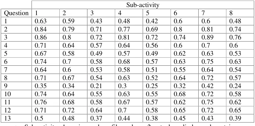
cate-gory good (2) for sub-activities. The

also not happy with the manner of

claim back by MSC with C2 smaller

than 50%. The pipe and profile and

tank, cylinder and container makers are

50 - 50 with technical support by

MSC. The sub-activities home

acces-sories makers, steel industries and

other user of the steel sheets have C2

less than 50% for the first question

(familiarity with MSC and its

pro-ducts). The results also show that all 8

sub-activities are happy with product

quality from the hot and cold rolling

sections of the MSC. The results (not

reported in here) show that almost 10%

and 21% of customers are happy (with

C2 greater than 60%) by the manner of

claim back and technical support of the

MSC. Figures 2 and 3 show the

pre-dicted cumulative probabilities for

response category good (y = 2) for all

202 customers. The results indicate

that almost 44% of the customers are

not happy with questions 1 (familiarity

with the MSC), 2 (dimensions

tole-rance by the hot rolling section) and 7

(dimensions tolerance by the pickling

section) with C2 less than 0.5.

6

.

Discussion

Two random component threshold

models are fitted to the customer’ s

opinion data. The threshold parameters

are independent of the question in the

first model whereas they are varying

by questions in the second model. The

models are called question independent

and question dependent random

com-ponent threshold models. The results

of the application indicate that the

thre-shold parameters do change

signifi-cantly over questions. Therefore, a

suitable model for analysing customer

satisfaction data is the question

depen-dent random components threshold

model. Question independent models

are led to a wrong decision about

factors in the model. The results of

question independent random

compo-nent threshold models indicate that

bet-ween two types of collecting data

whereas question dependent random

component threshold models do not

support such a conclusion.

We have also introduced a second

random component into the linear

pre-dicttor to allow possible change in

variance and pattern of association on

the second and following questions.

The results of application show that the

customer effect changes significantly

over questions. However, there is no

evidence of dependence between two

random components. Models lead to a

wrong decision about factors if the

significant random effects and

depen-dence between them are not included.

The estimation approach also provides

predicted values of random effects that

are very useful in identifying happy

and unhappy customers.

Appendix A

Let y be the observation vector of

the ordinal response variable Y. Let

be the corresponding vector of linear

combination of explanatory variables

and random components, given by

Zu

X ; u is the vector of

ran-dom components and X and Z are

regression and incidence matrices. Let

l1 be the log-likelihood function of y observations conditional on the value

of the random component vector u and

let l2 be the logarithm of the probability density function of u. The

functions l1 and l2 are

] |

| ln . )[ 2 / 1 (

ln

1 2

202 1

13 1 1

u A u

A

c

¦ ¦

const l

l _{i s} δ_is ∆_is

where

) G(

)

G( _{y is y 1 is}

is θ is η θ is η

∆ and

) G(

)

G( _{sy is s(y 1) is}

is θ is η θ is η

∆

under models (3.1) and(3.2)

respecti-vely. The δ_is is one if ith customer

uses product or service of the sth

ques-tion, zero otherwise. Penalised

likely-hood (PL) estimates ~, ~ and u~ are

obtained by maximising l = l1 + l2 with respect to , and u respectively.

initial step in finding ML and REML

estimates of ϕ_j and ϕ₃ via Anderson

(1973) and Henderson (1973)

algori-thm. The iterative procedure used to

obtain the ML and REML estimators

and their approximate

variance-covariance matrices can be specified as

follows:

(a) Let Iθ to be an identity matrix of dimension equal to the number of the rows

in _T, X* =

»¼ º «¬ ª Z X I 0 0 0

θ _{and k =0. Starting from initial values}

0, 0 , u0, ϕj0

and ϕ₃₀ (hence A0), the estimating equations are:

(3) » » » ¼ º « « « ¬ ª » ¼ º « ¬ ª c » » » ¼ º « « « ¬ ª » » » ¼ º « « « ¬ ª k k k k k k k k k u A V X V u u 1 0 1 1 1 * 1 1 1 1 0 0 / l / l ∂ ∂ ∂ ∂ where » » » ¼ º « « « ¬ ª ¸¸¹ · ¨¨© § » ¼ º « ¬ ª c c c c c 1 0 * 1 2 1 2 1 2 1 2 * 0 0 0 0 0 0 0 0 / / / / A X X V k k k k k k k k l l l l ∂ ∂ ∂ ∂ ∂ ∂ ∂ ∂ ∂ ∂ ∂ ∂ , k k k k k k k

k l l l l

l ∂ ∂ ∂ ∂ ∂ ∂ c ∂ ∂ ∂ c ∂ ∂ ∂ c

∂ / , / , / , / and 2₁/

1 2 1

2 1

1 are evaluated

at initial estimates of the parameters.

(b) Once iterations of (3) have converged to ~ and u~ , let ~ X~Zu~,

B ∂2l1/∂~∂~c, T* =[T*jj′]=[A−01+ZTBZ]−1, ajj′ =tr(T*jj′ +T*j′j)+2u~′j~uj′

andaj = tr(T*jj)+~u′j~uj for j ,j′=1 ,2.The ML estimates of ϕj and ϕ3 are

(4) ] 2 -[2 ˆ ] ) / ( ) / ( ) / ( [ ˆ 1 20 10 2 10 1 20 30 12 2 30 12 20 10 ) ( 3 30 2 30 2 30 1 ) ( − ′ ′ ′ ′ ′ − − + + = − + + = N a a a N a a N a a N ML jj j j j j j ML j ϕ ϕ ϕ ϕ ϕ ϕ ϕ ϕ ϕ ϕ ϕ ϕ ϕ ϕ ϕ ϕ

for j = 1, 2.

The preceding two steps are then repeated, with k =0, and initial values set to ~,

~_,

u~ , ϕ ˆ and

) ( 3

Once this iterative process has converged, the asymptotic variance-covariance matrix

for the ML estimators ϕ_ML (ϕˆ_1(ML) ,ϕˆ_2(ML),ϕˆ_3(ML))c is

(5) var( ) 2

>

@

jj jj jj

ML r r r

ϕ

where r1jj′ =tr[A(∂A/∂ϕj)A(∂A/∂ϕj′)]

,

and

)] / ( ) / ( [ *

3jj tr j j

r ′ = A ∂A ∂ϕ T ∂A ∂ϕ ′ .

Let           33 32 31 23 22 21 13 12 11 V V V V V V V V V

denote the

partitions of the matrix V

correspond-ding to the dimensions of , and u,

similarly let

          = − 33 32 31 23 22 21 13 12 11 1 T T T T T T T T T V .

Replacing 7* _{by T}

33 in (4) and (5) yields REML estimates ϕˆ_j(REML) and

) ( 3

ˆ_REML

ϕ and their corresponding

asymptotic variance-covariance matrix.

References

Anderson, T.W. (1973),

“Asymptotica-lly efficient estimation of

covarian-ce matricovarian-ces with linear structure,”

Annals of Statistics, 1 135 - 141.

Anderson, J. A. and Philips, P. R.

(1981), “Regression, discrimination

and measurement models ordered

categorical variables,” Journal of

Applied Statistics, 30, 22 - 31.

Breslow, N.E. and Clayton, D.G.

(1993), “Approximate inference in

generalised linear mixed models,”

Journal of the American Statistical

Association, 88,9 - 25.

Crouchley, R. (1995), “A random

effects model for ordered

category-cal data,” Journal of the American

Statistical Association 90, 489 -

498.

Gianola, D. and Foulley, I.J. (1983),

“Sire evaluation for ordered

catego-rical data with a threshold model,”

Genetics Selection Evaluation.

Harville, D.A. and Mee, R.W. (1984),

analysing ordered categorical data,”

Biometrics 40, 393 - 944.

Henderson, C.R.(1973b), Maximum

likelihood estimation of variance

components, unpublished

manus-cript.

Jansen, J. (1990), “ On the statistical

analysis of ordinal data when extra

variation is present,” Applied

Statistics 39, 75 - 84.

Jansen, J. (1992), “ Statistical analysis

of ordinal data from experiments

with nested errors,” Computational

Statistics & Data Analysis 13, 319 -

330.

McCullagh, P. and Nelder, J.A. (1989),

Generalized linear models. Second

Ed. London: Chapman and Hall.

McGilchrist, C.A. (1994), “ Estimation

in generalized mixed models,”

Journal of the Royal Statistical

Society, Series B 56, 61 - 69.

Nelder, J.A. and Lee, Y. (1996),

“ Hierarchical generalized linear

models,” Journal of the Royal

Statistical Society, Series B 58, 619

- 678.

Lee, Y. and Nelder, J.A. (2001a),

“ Hierarchical generalized linear

models: A synthesis of generalised

linear models, random effect model

and structured dispersions,”

Biomet-rika, 88, 987 - 1006.

Lee, Y. and Nelder, J.A. (2001b),

“ Modelling and analysing

corre-lated non-normal data,” Statistical

Modelling, 1, 3 - 16.

Saei, A. and McGilchrist, C.A. (1996),

“ Random component threshold

models,” Journal of Agricultural,

Biological and Environmental

Statistics, 1, 288 - 296.

Saei, A. and McGilchrist, C. (1998),

“ Longitudinal threshold models with

random components,” The

Statisti-cian , Series D 47, 365 - 375.

Schall, R (1991), “ Estimation in

generalised linear models with

ran-dom effects,” Biometrika 78, 719 -

Ten Have T. (1996), “ A mixed effects

model for multivariate ordinal

response data including correlated

discrete failure time with ordinal

responses,” Biometrics, 53, 473 -

491.

Wolfinger, R. (1993), “ Laplace’ s

approximation for nonlinear mixed

models,” Biometrika 80, 791 - 796.

Zhaorong, J., McGilchrist, C.A. and

Jorgensen, M.A. (1992), “ Mixed

model discrete regression,”

Biomet-rical Journal34, 691 - 700.

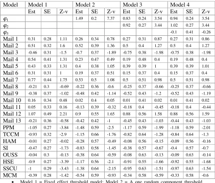
Table 1: REMLestimate of parameters (Est), standard error (SE) and Z-v = (Est/SE).

Model Model 1 Model 2 Model 3 Model 4

Est SE Z-v Est SE Z-v Est SE Z-v Est SE Z-v

ϕ1 1.49 0.2 7.37 0.83 0.24 3.54 0.94 0.24 3.54

ϕ2 0.92 0.27 3.44 1.02 0.27 3.44

ϕ3 -0.1 0.41 -0.26

Mail 1 0.31 0.28 1.11 0.26 0.34 0.78 0.27 0.31 0.87 0.27 0.31 0.86

Mail 2 0.51 0.32 1.6 0.52 0.39 1.36 0.5 0.4 1.27 0.5 0.4 1.27

Mail 3 -0.46 0.31 -1.5 -0.7 0.37 -1.89 -0.75 0.38 -1.98 -0.75 0.38 -1.98

Mail 4 0.54 0.41 1.31 0.23 0.47 0.49 0.19 0.48 0.4 0.19 0.48 0.4

Mail 5 0.43 0.33 1.31 0.4 0.38 1.05 0.39 0.39 1 0.39 0.39 1.01

Mail 6 0.31 0.31 1 0.19 0.37 0.51 0.15 0.37 0.4 0.15 0.37 0.4

Mail 7 0.77 0.44 1.75 0.53 0.5 1.08 0.5 0.51 0.98 0.5 0.51 0.98

Mail 8 -0.21 0.3 -0.69 -0.22 0.36 -0.6 -0.25 0.37 -0.66 -0.25 0.37 -0.66

Mail 9 -0.38 0.37 -1.02 -0.48 0.42 -1.14 -0.52 0.43 -1.2 -0.52 0.43 -1.19

Mail 10 0.16 0.34 0.48 0.02 0.4 0.05 0.01 0.41 0.02 0.01 0.41 0.02

Mail 11 0.05 0.33 0.16 -0.13 0.39 -0.32 -0.18 0.4 -0.45 -0.18 0.4 -0.44

Mail 12 1.07 0.49 2.21 0.9 0.55 1.65 0.88 0.56 1.58 0.88 0.56 1.59

Mail 13 -0.21 0.36 -0.58 -0.42 0.42 -1 -0.45 0.43 -1.03 -0.44 0.43 -1.03

PPM -1.05 0.27 -3.84 -1.48 0.59 -2.5 -1.17 0.59 -1.99 -1.18 0.59 -2.01

TCCM -0.93 0.32 -2.9 -1.15 0.66 -1.76 -0.82 0.64 -1.28 -0.84 0.64 -1.3

HAM -0.01 0.27 -0.02 -0.28 0.57 -0.49 -0.08 0.56 -0.15 -0.09 0.56 -0.16

SI -0.47 0.27 -1.73 -0.83 0.58 -1.45 -0.38 0.57 -0.67 -0.4 0.57 -0.7

OUSS -0.04 0.3 -0.13 -0.38 0.64 -0.59 -0.08 0.63 -0.13 -0.09 0.63 -0.14

HSE -0.9 0.27 -3.39 -1.17 0.56 -2.1 -0.91 0.55 -1.66 -0.92 0.55 -1.68

SSCU -1 0.29 -3.43 -1.38 0.64 -2.15 -0.95 0.63 -1.51 -0.97 0.63 -1.54

MCM -0.39 0.28 -1.42 -0.54 0.59 -0.93 -0.34 0.58 -0.59 -0.33 0.58 -0.6

x Model 1 = Fixed effect threshold model; Model 2 = A one random component threshold model; Model 3 = A two independent random components threshold model; Model 4 = A two random components threshold model

x Mail i is the mail effect for the question i, i = 1, 2,… , 13

x Water, oil and gas pipe makers and face – face effects are fixed at zero for identifiably x PPM = pipe and profile makers, TCCM = tank, cylinder and container makers, HAM = home

Table 2: REML predicted probability and cumulative probability of the response categories.

Category Cumulative

Question 1 2 3 4 C1 C2 C3

1 0.09 0.43 0.38 0.1 0.09 0.52 0.9 2 0.3 0.46 0.22 0.02 0.3 0.76 0.98 3 0.3 0.47 0.2 0.03 0.3 0.77 0.97 4 0.19 0.43 0.25 0.13 0.19 0.62 0.87 5 0.21 0.35 0.31 0.12 0.21 0.56 0.87 6 0.2 0.44 0.26 0.09 0.2 0.64 0.9 7 0.14 0.42 0.33 0.11 0.14 0.56 0.89 8 0.18 0.44 0.27 0.12 0.18 0.62 0.89 9 0.06 0.23 0.36 0.35 0.06 0.29 0.65 10 0.1 0.54 0.31 0.05 0.1 0.64 0.95 11 0.09 0.55 0.34 0.02 0.09 0.64 0.98 12 0.08 0.58 0.33 0.01 0.08 0.66 0.99 13 0.11 0.32 0.27 0.31 0.11 0.43 0.7

x Category: 1 = very good, 2 = good, 3 = not bad and 4 = bad

x Cumulative: C1 = P(Y ≤ 1), C2 = P(Y ≤ 2) and C3 = P(Y ≤ 3).

Table 3: REML predicted cumulative probability of the second category, (good), for 8 sub-activities.

Sub-activity

Question 1 2 3 4 5 6 7 8

1 0.63 0.59 0.43 0.48 0.42 0.6 0.6 0.48 2 0.84 0.79 0.71 0.77 0.69 0.8 0.81 0.74 3 0.86 0.8 0.72 0.81 0.72 0.74 0.89 0.76 4 0.71 0.64 0.57 0.64 0.56 0.6 0.7 0.6 5 0.67 0.58 0.49 0.57 0.49 0.62 0.63 0.53 6 0.74 0.7 0.58 0.68 0.57 0.63 0.75 0.63 7 0.64 0.6 0.53 0.58 0.51 0.55 0.64 0.54 8 0.71 0.67 0.54 0.63 0.52 0.64 0.72 0.57 9 0.35 0.34 0.21 0.3 0.25 0.32 0.42 0.24 10 0.74 0.64 0.55 0.63 0.55 0.68 0.72 0.58 11 0.76 0.68 0.58 0.67 0.57 0.62 0.75 0.62 12 0.71 0.72 0.64 0.7 0.58 0.65 0.72 0.65 13 0.5 0.48 0.37 0.44 0.38 0.45 0.43 0.39

Figure 1: REML estimates of the threshold parameters on each 13 questions.

-4 -1 2 5

1 2 3 4 5 6 7 8 9 10 11 12 13

Question

E

st

im

at

e _{Theta 1}

Theta 2 Theta 3

Figure 2: REML predicted cumulative probability of the response category 2 ( P(Y≤2)) for the question 9 (the manner of claim by MSC).

0 0.4 0.8

1 52 103 154

Customer

Pr

ed

ic

te

d

V

al

u

e

Figure 3: REML predicted cumulative probability of the response category 2 ( P(Y≤2)) for the question 13 (Technical support by MSC).

0 0.4 0.8

1 52 103 154

Customer

Pr

ed

ic

te

d

V

al