The Second Birth Interval in Egypt: The Role of Contraception
Angela Baschieri
Abstract
The paper discusses problems of model specification in birth interval analysis. Using
Bongaarts’s conceptual framework on the proximate determinants on fertility, the paper tests
the hypothesis that all important variation in fertility is captured by differences in marriage,
breastfeeding, contraception and induced abortion. The paper applies a discrete time hazard
model to study the second birth interval using data from the Egyptian Demographic and
Health Survey 2000 (EDHS), and the month by month information on contraceptive use,
breastfeeding, and postpartum amenorrhea available in the EDHS calendar. The paper shows
the importance of including both information on contraceptive use by types, breastfeeding,
and postpartum amenorrhea period in birth intervals analysis.
The Second Birth Interval in Egypt:
The Role of Contraception*
Angela Baschieri
School of Social Sciences University of Southampton
United Kingdom
Abstract
The paper discusses problems of model specification in birth interval analysis. Using Bongaarts’s conceptual framework on the proximate determinants on fertility, the paper tests the hypothesis that all important variation in fertility is captured by
differences in marriage, breastfeeding, contraception and induced abortion. The paper applies a discrete time hazard model to study the second birth interval using data from the Egyptian Demographic and Health Survey 2000 (EDHS), and the month by month information on contraceptive use, breastfeeding, and postpartum amenorrhea available in the EDHS calendar. The paper shows the importance of including both information on contraceptive use by types, breastfeeding, and postpartum amenorrhea period in birth intervals analysis.
* Angela Baschieri, Division of Social Statistics, School of Social Sciences, University of Southampton, Southampton SO17 1BJ, United Kingdom; E-mail:
According to the 2000 Egyptian Demographic and Health Survey(EDHS), few
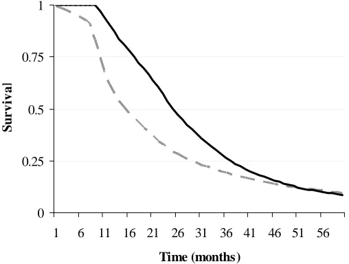
women who approve of family planning think that a newly married couple should use contraception to delay the first birth and only 0.3% of currently married women use modern methods of contraception before their first birth (El-Zanaty and Way 2001). More than 50% of married women conceive their first child in less than six months from the marriage date and in just over a year and half 75% do so. Among those women in the EDHS who had a first child, 50% conceived the second child within a year and half of the birth of the first child, and it took almost two years and a half for 75% of them to conceive their second child (Figure 1), the first birth interval is shorter than the second and contraceptive use appears not to play a role in determining its length. Women start using contraception after the first birth.
It has been suggested that the reproductive process, starting from the second birth, is like an engine with its inbuilt momentum, and early behaviour shapes the rest of the childbearing experience (Rodriguez et al. 1984). Hence studying the second birth interval may shed light on subsequent birth intervals and on fertility differentials in general.
Figure 1 about here
This paper studies the dynamics of the second birth interval in Egypt. I use data from the 2000 EDHS that provide information about fertility and family planning, also monthly calendar data on contraception, breastfeeding and postpartum
that it provides fairly reliable information. A discrete-time survival model has been applied, introducing information on breastfeeding, postpartum amenorrhea and types of contraceptive use in the form of time-varying covariates, which allowing the detection of changes in the discrete-time hazard rate because of the timing of the use of contraception, breastfeeding behaviour and postpartum amenorrhea.
In the first section of this paper I present the background of the study and introduce the problem of model specification of time to birth data. In the second section I introduce the conceptual framework. The third section presents the data and consideration issues of sample selection. The fourth section presents the methodology, and the fifth section presents the major results.
BACKGROUND
Several studies (Rodriguez et al. 1984; Trussell et al. 1985) have found the length of the previous birth interval a strong determinant of the duration of the subsequent birth interval. Rodriguez et al (1984) found that birth intervals for specific women result from a persistence of behavioural or biological traits over time. They found that the birth interval length depends little upon birth order, but far more upon the length of the previous interval. They stated that, starting at least from the second birth, it appears that the reproductive process can be encapsulated as an ‘engine with its own in built momentum’(Rodriguez et al. 1984:5), and early behaviour and
childbearing experience starts, and in Egypt few newly married couples use contraception to space the first birth interval.
By comparing results of identical structural models for nine countries,
Rodriguez et al. (1984) found that, together with the length of the previous interval, the women’s education, age and time period all had substantial effects on birth interval length. Richards (1983) incorporated in her analysis both duration of breastfeeding and contraception, although she did not include the length of the previous interval or monthly information about contraception use, as in the World Fertility Survey (WFS) calendar types of information were not collected. The only contraceptive information available in the WFS was whether or not a woman used contraception in each birth interval. Subsequent work by Trussell et al. (1985) did include in a model both information on breastfeeding, the length of the previous interval and contraception, but as in the case of Richards (1983), they did not have month by month information about breastfeeding. Rindfuss, Palmore and Bumpass (1987) analyzed the determinants of birth interval length for five countries, using WFS data. The important effects they found were those due to the age of mother at first birth, urban experience, and (for Korea) sex of preceding child. Notably, they found that respondent’s education was unimportant. McDonald and Egger (1990), analysing the first birth interval using the Portugal Fertility Survey, in which they did have information about duration of contraceptive use for the last closed birth interval, found a significant effect of contraceptive use on the risk of conception, although they were looking at the first birth interval and not at the role of contraception in shaping the whole reproductive process.
due to important variables being omitted from the model. So far as data availability is concerned, the problem arises not just because information is not being collected, but also because the information that is collected is not accurate enough. For example, to study the determinants of birth interval length one would ideally need information about fecundability, intensity of breastfeeding, and contraceptive use over time, as well as detailed information about such socio-economic variables as are likely to affect the risk of conception over time (for example respondent’s work status and educational level at each time point). Unfortunately, only rarely does a study designed to look at fertility and family planning in developing countries collect information in longitudinal format. For these reasons researchers are often constrained to study the dynamics of fertility and family planning using cross-sectional surveys.
As far as the problem of model specification in duration analysis is concerned, several authors (Blossfeld and Rohwer 1995; Rindfuss et al. 1987) have stressed the fact that the exclusion of important covariates is likely to create misspecification in the model and provide an incorrect estimate for the shape of the hazard with respect to time. For example, duration of breastfeeding was commonly omitted until recently, and it might be that there are still other important intermediate variables which are presently unnoticed. Researchers have tried to cope with this problem of important omitted variables in the model by introducing an error term, and in duration analysis the residual becomes an important part of the model specification. Despite this theoretical rationale for introducing error terms in duration model, in the literature there are still opposing views about the appropriateness of their use(see below for further discussion).
with high contraceptive use recent DHSs have collected retrospective monthly information about contraception, breastfeeding and postpartum amenorrhea for five years before the survey date. This study therefore makes use of the most detailed information available in DHS for countries with high contraceptive use. The
introduction of month by month information on contraception will allow us to detect changes in the discrete time hazard rate because of the timing of use of contraception by types, breastfeeding behaviour and post partum amenorrhea. The study uses a discrete-time hazard model accounting for unobserved heterogeneity that is gamma distributed, and discusses the implications of the shape of hazard and survival function because of the introduction of the error term
CONCEPTUAL FRAMEWORK
In a well known article, Bongaarts (1982), using aggregate analysis with countries as units, demonstrated that virtually all important variation in fertility is captured by differences in marriage, breastfeeding, contraception, and induced abortion. He showed that the explained variance, using the estimated total fertility rates to predict the actual total fertility rates, was 0.96, a remarkable success for any social science model, even one using aggregate data (Rindfuss et al. 1987). Because of these results it seems reasonable to ignore other intermediate variables in data analysis. The conventional theoretical wisdom regarding the way in which socio-economic
Against this background, individual-level analyses of birth intervals have been reaching different results. Many authors have still found direct effects of socio-economic variables on the dynamics of birth interval after controlling for proximate variables (Bumpass, Rindfuss and James 1986; Palloni 1984; Trussell et al. 1985). Rindfuss et al. (1987) argue that there could be three possible explanations for the discrepancy between theory and empirical micro level analysis. One is that the conventionally-used measures of the four proximate determinants of fertility are inadequate operationalizations of the theoretical constructs. For example if a substantial proportion of all contraceptive use were not reported, observed contraceptive use patterns would miss much of contraception’s mediating role. Second, it is possible that there could be specification errors due to the omission of important intermediate variables (Kallan and Udry 1986). Third, the effects of some of the intermediate variables or the socioeconomic variables might be curvilinear rather than linear.
Figure 2 about here
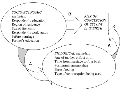
The biological variables in Figure 2 consist of those variables that in
Bongaarts’s (1982) conceptual framework were defined as proximate variables. As I wish to discover if their role is an intermediate one or not, to avoid confusion I shall refer to them as biological variables. Among the biological variables I did not include abortion as abortion in Egypt is only allowed if it considered necessary to save the life of mother and in no other circumstances. Therefore abortion cannot be considered in Egypt as a measure of birth control. The biological variables include both
breastfeeding and postpartum amenorrhea. The contraceptive effect of breastfeeding changes over time. It is greatest in the period of postpartum amenorrhea but can continue at lower intesity even after the period of amenorrhea has finished. Among the biological set of variables we also include month by month information on
contraceptive use by methods and information on the length of time elapsing between marriage and the first birth. Only 0.3% of married women in the EDHS used
contraception before the birth of their first child, the length of the first birth interval is likely to be largely determined by a couple’s fecundity. Finally amongst the
biological variables we include age at first birth, for its interacting effects with the other biological variables.
of endogeneity relating to current work status. A similar rationale is applied for the respondent‘s level of education at first birth, which has been calculated considering the Egyptian educational system (see note to Table 1). I include husband’s educational level at the time of respondent’s first birth to capture the effect of husband’s socio-economic level.
Separate consideration is needed of the effect of duration since first birth on the risk of conception of the second child. Intuitively the risk of conception will be very low for the first month or two from conception and increase and decrease thereafter. However, it is not clear exactly what status duration has in this conceptual framework and, whether indeed, its effect still exists after controlling for other socio-economic variable and biological variable. We will then consider duration as a variable in our model and test if its effect is significant after accounting for the other covariates (allowing for a flexible specification of its possible effects).
DATA AND SAMPLE SELECTION
the first row usually representing January of the fifth calendar year before the survey (for the 2000 EDHS, it represents January 1995). The columns are used to record different types of information for each month. In the 2000 EDHS calendar there are six columns. The first column contains month by month information about births, pregnancies and contraception, the second contains information about the reasons for discontinuation of contraceptive methods, the third about marriages and unions, the fourth about sources of family planning methods, the fifth about postpartum
amenorrhea and the sixth about breastfeeding.
Studies of the quality of the DHS calendar data on contraceptive have shown that they are fairly reliable (for Brazil see Leone (2002). Strickler et al. (1997) had the unique opportunity to use data from 1995 Morocco Panel Survey to evaluate the reliability of the contraceptive history data collected in the calendar of the 1992 DHS. Since the Panel Survey consisted of a sub-sample of respondents from the calendar DHS. Both surveys included a five-year calendar, and the two calendars overlap for the period 1990-92. Strickler et al. (1997) found that the reporting of contraceptive use was fairly reliable, though they found that data on contraceptive discontinuation and on complex histories were mare unreliable. These findings suggest that
contraceptive use information is overall fairly robust though estimates of
contraceptive failure rates are likely to be less accurate than estimates of prevalence. In the present analysis I selected all women who had their first birth after the beginning of the calendar (January 1995) a total of 2899 women, I excluded
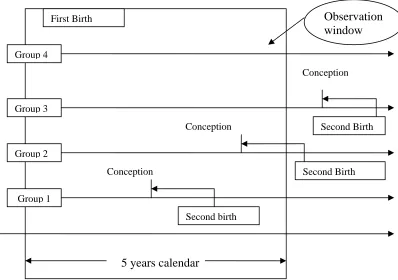
The event of interest is the conception leading to the second live birth. There are four possibilities (Figure 3): (1) the second birth occurs within the calendar period, (2) the second birth is after the survey date but conception happened before the survey date, (3) the second birth is conceived after the survey date, (4) there was no second conception even after the survey date. For the first group of women (who had a
second birth within the calendar period) the time to conception is the time between the birth of first child and the birth of the second minus nine months. The event variable takes the value of 1 in the month that the second conception leading to a live birth occurs. The second group consists of women that conceived the second child before the end of the calendar but the birth happened after the survey date. For these women I use the information on pregnancy history in order to time the event conception leading to a live birth. I assume that if a woman is pregnant for at least three months before the end of her calendar then the pregnancy will lead to the second live birth and the event variable takes the value of 1 in the month of conception. In this way we will also allow for miscarriage, since most miscarriages are in the first three months of pregnancy. For women who conceived their second child after the survey date the duration is calculated between the birth of first child and a point three months before the survey date. In this case the event variable takes the value of 0 as the conception leading to a live birth did not occur within the period of observation. The same applies for those women that will never conceive a second child. In our sample, out of 2899 women, 1684 conceived their second child during the study period.
Figure 3 about here
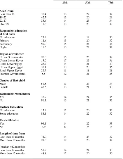
25th, 50th, and 75th percentiles of the second birth interval in months by selected background characteristics. In other words column 2 shows the number of months by which 25% of the relevant subgroup of women had their second birth, column 3 shows the number of months by which the 50% of the same women had their second birth, column 4 the number of months by which 75% had their second birth.
Table 1 about here
The mean length of time from marriage to birth of the first child is 19 months for the women in our sample. Among women for whim the length of time from marriage to the first child is less than the mean the length of the second birth-conception interval is longer. The same applies if instead of the mean we use the median birth interval (12 months). I return to this issue later.
METHOD
In the present analysis I apply a discrete time hazard model of the length of time between first birth and the conception leading to the second live birth. This model specification will allow for a flexible baseline hazard, so there is no need to assume a functional form of the effect of duration. The duration will be broken into k categories (say 0-2 months, 3-5 months, etc…) during which the risk of pregnancy is assumed constant for individuals with the same values of the covariates. The degree of flexibility of the baseline hazard will depend on the number of duration dummies in the models.
The discrete time hazard rate is defined as:
hit = prob[Ti =t|Ti ≥t,xit] , (1)
where is a vector of regressor variables (covariates), some of which can be fixed covariates, and others can be time-varying. is a discrete random variable
representing the time at which the end of the spell occurs.
it x
i T
person-months format, the model likelihood has exactly the same form as that for a standard binary logit regression model. Furthermore this model specification will facilitate the introduction of time-varying covariates in the model. This type of model also allows for censoring in the data.
The hazard rate is defined as follows:
hit =1/{1+exp[−θ
( )
t −β'xit]}⇔log[hit/(
1−hit)
]=θ( )
t +β'xit, (2)
where θ(t)allows the hazard to vary with time. As has been previously mentioned this specification facilitates the inclusion of time-varying covariates, since can include both time-varying and fixed covariates. Furthermore the time varying
covariates and fixed covariates can have fixed effects as well as time-varying effects.
it x
In the present analysis I treated breastfeeding practices, postpartum amenorrhea, and contraception as time-varying covariates with fixed effects, and all the other variables as fixed covariates with fixed effects. During the analysis several interactions of fixed-effect variables and time-varying variables with duration
The particular model estimated accounted for unobserved heterogeneity, the hazard rate being defined as:
log
[
hit /(1−hit)]
=θ(t)+β'Xit +εi (3)The two models are estimated using the pgmhaz command in STATA
developed by Jenkins (1997). This command estimates, by maximum likelihood, two discrete time grouped duration data proportional hazard models one of which
incorporates a gamma mixture distribution to summarize individual unobserved heterogeneity (or ‘frailty’). The two models estimated are : (1) the Prentice and Gloecker (1978) model ; and (2) the Prentice and Gloecker (1978) model
incorporating a gamma mixture distribution to summarize unobserved individual heterogeneity, as proposed by Meyer (1990). The Prentice-Gloeckler-Meyer models estimated are described by Stewart (1996).
As previously mentioned, in the literature there is diverging opinion about the value of including unobserved heterogeneity in the model. Some authors argue
(Jenkins 1997; Lancaster 1979) that failing to account for unobserved heterogeneity in the model will result in a over-estimation of the degree of negative duration
at longer durations. Moreover, failing to account for unobserved heterogeneity will bias the parameter estimates of regressors as well.
Although there are strong positive arguments for the inclusion of unobserved heterogeneity in the model, some authors (Blossfeld and Rohwer 1995) have argued that a drawback of accounting for unobserved heterogeneity in the model is that the parameter estimates can be highly sensitive to the assumed parametric form of the error term. As an example Heckman and Singer (1982) estimated four different unobserved heterogeneity models: one with a normal, one with a log-normal, and one with a gamma distribution of the error term, as well a model with a non-parametric specification of the disturbance. They found that the parameter estimates provided by these models were surprisingly different. In other words, as Blossfeld and Rohwer (1995) suggest, the identification problem might only be shifted to another level. The misspecification of the duration variables caused by neglecting the error term might be replaced by misspecification of the parametric distribution of the error term.
On the other hand others suggest that if with a flexible specification of the duration dependence, i.e. in our case the 10 duration dummies, the misspecification can be avoided. McDonald and Egger (1990) have suggested that the unobserved heterogeneity in the analysis of birth intervals could allow us to measure individual fecundity. As individual fecundity varies from couple to couple and it is inherently not observable or reportable, including unobserved heterogeneity in the model will having to assume that there are no omitted covariates in the model, and will also allow measurement of individual unobserved fecundity.
the purposes of comparison and I discuss the implications of the introduction of unobserved heterogeneity in the model.
RESULTS
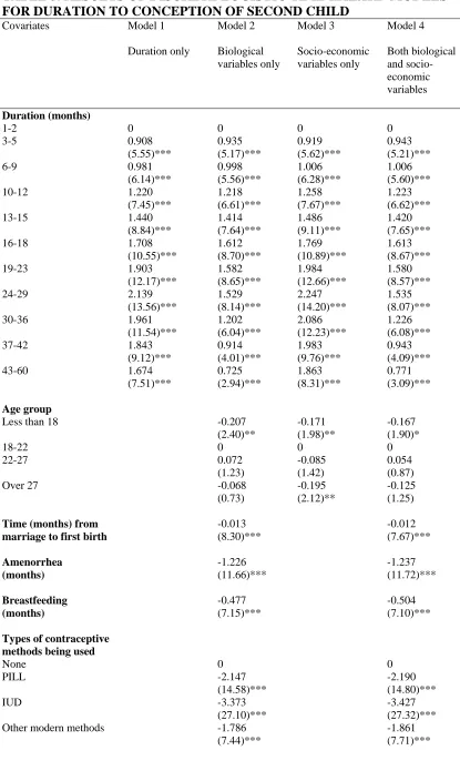
As previously stated I estimate four different models. Model 1 includes only duration, and tests whether the raw hazard varies with duration since the first birth. Model 2 includes only the biological variables that have been shown to affect fertility (age of mother at first birth, breastfeeding, amenorrhoea, use of types of contraception, and the length of the interval between marriage and first birth). Model 3 includes only socio-economic variables (region of residence, respondent’s education, husband’s education, whether or not the respondent worked before marriage, and sex and survival status of the first child). Model 4 includes both the socio-economic variables and biological variables. In this way I can compare the ‘socio-economic’ model to the ‘biological’ model, determining which one performs better after having accounted for contraception as a time-varying covariate in the ‘biological’ model.
In the presentation of the results I shall use two statistics employed by Rodriguez and Hobcraft (1983) in their illustrative analysis of life tables. As
(
q1 2q2 q3)
4T = + +
,
where T is the trimean and , , and are the durations by which 25, 50 and 75% respectively of those women who go on to have their next child within five years have had their next child. When the right tail is long, as is true for the distribution of
pregnancies in a birth interval, the trimean will be higher (slightly) than the median. Rodriguez and Hobcraft (1983) considered the birth interval length and calculated the quintum and trimean for each parity.
1
q q2 q3
In the present study I shall modify the definition, following Trussell, Vaughan and Farid (1988). In their work on birth intervals in Egypt using the 1980 Egyptian Fertility Survey, they considered the birth-pregnancy interval (from the birth of a child to the conception of the following one) instead of the inter-birth interval (from birth of a child to the birth of the following one). Hence, the quintum is the estimated proportion becoming pregnant within 51 months and is a direct estimate of the proportion giving birth within five years, and the trimean is a measure of the average birth-pregnancy interval of those women who conceived their second child within 51 months of giving birth to their first. Other measurements that could be calculated to report the dispersion of the data include the spread (or inter-quartile range). The spread, in this case, is the difference between the duration by which 25% of women conceive their second child and the duration by which 75% of women conceive their second child.
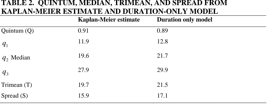
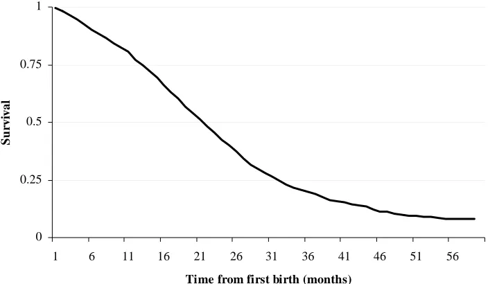
child within 51 months, with an average first birth-pregnancy interval of almost 20 months. Furthermore 25% of women conceive their second child within a year (11.9 months) and 50% of women in just over a year and a half (19.6 months).
Figure 4 about here
Table 2 about here
Biological and socio-economic models
The results from Models 1 to 4 are shown in Table 3. Consider first Model 1, with only duration as a covariate. Figure 5 shows the shape of hazard of conception for this model, and demonstrates that the risk of conceiving the second child increases almost monotonically until two years after the birth of the first child, and then
decreases. The quintum of this ‘duration-only’ model is 0.89 (89% of women became pregnant within 51 months) and the trimean is 21.6.
Figure 5 about here
Table 3 about here
reduces the risk of conception even among non-amenhorreic women. The use of contraception greatly decreases the hazard of conception, with the IUD being slightly more effective in this respect than the pill or other methods.
Model 3, which includes only socio-economic variables, has a much lower explanatory power than Model 2. Although several socio-economic variables
significantly affect the hazard in Model 3, in all but one case the effects are reduced in magnitude in Model 4, which includes both biological and socio-economic variables. However, Model 4 does mark a significant improvement on the ‘biological-only’ model (Model 2). Performing a likelihood-ratio test we have:
(2{Log-Likelihood (full model) - Log-Likelihood (biological only model)} = 2 x (-6031)-(-6004)
= 54
with 12 degree of freedom (p < 0.0005). Model 4 with both socio-economic variables and biological variables thus performs better than the ‘biological only’ model.
Looking at the effect of socio-economic variables in Model 4 on the risk of conception we can see that the respondent’s and husband’ education, whether or not the respondent worked before marriage, the sex of the first child, and region of residence have a significant effect on hazard of conception after controlling for
before marriage the monthly hazard of conception of second child decreases by 17%, resulting in a longer birth interval. If the partner of the respondent has some level of education the monthly hazard of conception increases by 28%, resulting in a shorter birth interval.
One possible explanation of the continued significance of some socio-economic variables in the model after the biological variables have been included is that,
although the framework of Bongaarts (1982) still holds in general, including the socio- economic variables improves our measurement of the impact of intermediate variables. For example, if the first child is a boy, one would expect more
contraceptive use because of a reduced need to have a second child quickly compared to the situation when the first child is a girl. However the ‘sex-of-first-child’ effect is still significant after accounting for contraceptive use and duration of breastfeeding. This might be because, for example, boys are breastfed more intensely than girls, or that contraception is used more carefully after a boy than a girl. The same could be said about women with higher education and husbands with some level of education. Women with higher education may have the potential to use more effective
contraceptive methods and reduce the failure rate of contraception. The partner’s level of education could be considered as a proxy for the socio-economic status of
household, and a household with higher socio-economic status could afford better medical advice as well understand better how certain contraceptive methods work, reducing the failure rate.
of the first child appears to be strongly negative. One possible explanation of this is that while the first child survives, women rely on breastfeeding for contraception, whereas if the child has died women are compelled to switch to appliance or
hormonal methods, which are more effective than breastfeeding, and thus reduce their monthly risk of conception. To test this, I added to Model 3 a term measuring the interaction between the duration and the survival status of the first child. The results (not shown) were consistent with this account, in that the effect of the death of the first child was greatest at those durations where the surviving children were being breastfed less intensely, and the contraceptive effect of breastfeeding was gradually being eroded.
This gradual erosion of the contraceptive effect of breastfeeding as the first child grows up also explains why no multicollinearity problem exists with the introduction in the model of both breastfeeding information and the period of postpartum amenorrhea. Therefore, it is important to include both information on breastfeeding and postpartum amenorrhea in model specification in birth interval analysis. In addition, no multicollinearity problem appears also to exist between respondent’s and husband’s educational level, and between respondent’s work status before marriage and respondent’s level of education.
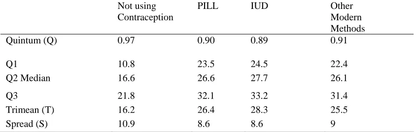
Figure 6 shows the shape of the hazard for four types of women: (1) a woman that did not breastfeed, who was never subject to post-partum amenorrhea and who did not use contraception over the study period; (2) a woman who used the pill but did not breastfeed and was never subject to post-partum amenorrhea; (3) a woman who used the IUD, did not breastfeed and who was never subject to post-partum
that the shapes of the hazards displayed below refer to hypothetical women, Figure 6 helps reveal the effectiveness of different types of contraceptive method. The IUD is the most effective method of contraception, whereas the pill is a less effective method.
Figure 6 about here
Figures 7 and 8 show the hazard and survivor functions of four more ‘realistic’ groups of women. All these groups of women were both breastfeeding and
amenorrheic for the first four months after the birth of the first child. After this the amenorrhea ceased, but they kept on breastfeeding until month 13 after the first child was born. The first group did not use contraception at all during the observation period. The second group used the IUD for 18 months after the period of amenorrhea ended (they were both breastfeeding and using contraception for nine months, after which they continued to use the IUD for other 9 months). The third and fourth groups are like the second group, except that they used the pill and ‘other modern methods’ respectively instead of the IUD.
Figure 7 about here
Figure 8 about here
Table 4 about here
Effect of length of first interval and contraception on the second birth
interval.
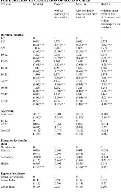
I estimated three additional models to show the changes in the effect of other covariates on the hazard of conception of second birth after having excluded the contraception variables, and to assess if the effect of the length of the interval between marriage and birth (the first birth interval) is linear and if this effect changes with the exclusion of contraceptive use variables. Model 5 is the same as Model 4 but without the contraceptive use variables. Model 6 is a variation of Model 4 in which the length of the first birth interval is allowed to have a non-linear (quadratic) effect on the hazard. Model 7 is, in effect, a combination of Models 5 and 6, in that it both excludes the contraceptive use variables and allows the length of the first birth interval to have a quadratic effect.
Comparing Models 4 and 5, there are changes in the effect of several socio-economic covariates when contraceptive use is excluded. Without the contraceptive use variables, the effect of having a secondary education is significant, whereas the effect of having higher education becomes insignificant, The effect of being resident in rural Upper Egypt and Frontier Governorates and the survival status of first child are significant when contraceptive use is excluded, but not when it is included. The opposite is true of husband’s education. These results confirm the importance of accounting for contraceptive use practises in the study of birth intervals, but also that socio-economic variables do have something to add to the explanatory power of a model over and above the contribution made by the proximate determinants.
Table 6 about here
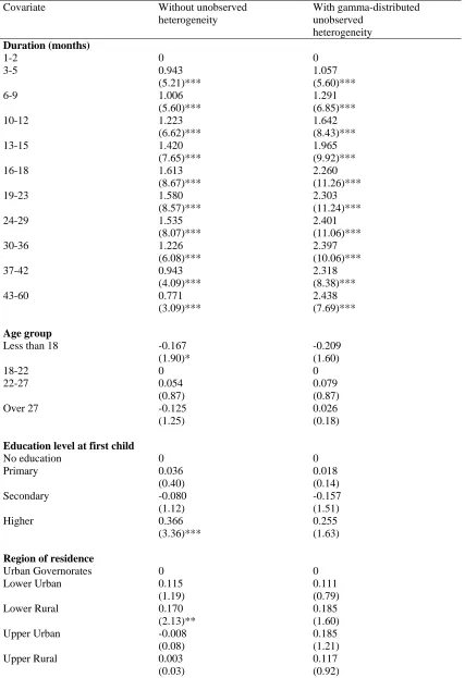
Unobserved heterogeneity
Finally, I estimated Model 4 (the combined model) incorporating a term for gamma-distributed unobserved heterogeneity. The results (Table 6) show that the unobserved heterogeneity parameter is significant suggesting that individual-level unobserved heterogeneity should be part of the model.
Comparing the two models in Table 6, it is seen that in the model with
result that different duration segments contain women with similar levels of
unmeasured risk. Moreover, once we account for unobserved heterogeneity all the socio-economic variables except husband’s education lose their significance, whereas biological variables as amenorrhea and contraceptive use become more significant.
Table 7 about here
Figure 9 about here
CONCLUSION
Using data from Egyptian Demographic and Health Survey (EDHS), and the month by month information on breastfeeding, post-partum amenorrhea and contraceptive use by method available in the EDHS calendar, this paper has looked at the
determinants of the second birth interval in Egypt. The results of analysis
demonstrate the importance of introducing this kind of information on contraception in birth interval analysis. They also show that we should not only include in the analysis the period of breastfeeding but also the period of post-partum amenorrhea.
model which does not control for unobserved heterogeneity. However, when unobserved characteristics are controlled for by incorporating a heterogeneity term, the direct impact of socio-economic variables on the hazard of conception becomes very small.
Despite the fact that the analysis reported in this paper was not designed to study contraceptive failure rates, it can help to provide a picture on contraceptive failure in Egypt. The results of the analysis of the second birth interval in Egypt show a degree of failure of contraceptive use. The level of contraceptive failure varies by method, though a degree of failure is present in every method of contraceptive use. It seems that in Egypt the IUD is less prone to failure than the pill or other model methods. Results suggest that policy makers should not only look at increase uptake of contraceptive methods but improve family planning counselling, as contraceptive methods have still a high degree of failure, suggesting an improper assistance from Family Planning providers in providing adequate information.
REFERENCES
Bumpass, L.L., R.R. Rindfuss, and P. James. 1986. "Determinants of Korean Birth Intervals: The Confrontation of Theory and Data." Population Studies 40(3):403-423. El-Zanaty, F.and A. Way. 2001. "Egypt Demographic and Health Survey 2000." Calverton, Maryland (USA): Ministry of Health and Population (Egypt),
National Population Council, ORC Macro,.
Heckman, J.J.and B. Singer. 1982. "The identification Problem in Econometric Models for Duration Data." Pp. 39-77 in Advances in econometrics, edited by W. Hildenbrand. Cambrigde: Cambrigde University Press.
Hobcraft, J.and J. McDonald. 1984. "Birth Intervals." in Comparative Studies. London: World Fertility Survey.
Jenkins, S.P. 1995. "Easy Estimation Methods for Discrete-Time Duration Models."
Oxford Bulletin of Economics and Statistics 57(1):129-138.
—. 1997. "Estimation of Discrete Time (grouped duration data) Proportional Hazards Models: pgmhaz." in Mimeo: ESRC Research Centre on Micro-Social Change, University of Essex.
Kallan, J.and J.R. Udry. 1986. "The Determinants of Effective Fecundity Based on the First Birth Interval." Demography 23(1):53-66.
Lancaster, T. 1979. "Econometric Methods for Duration of Unemployment."
Econometrica 47(4):939-956.
Leone, T. 2002. "Fertility and Union Dynamics in Brazil." Unpublished doctoral dissertation, Department of Social Statistics, University of Southampton.
McDonald, J.and P.J. Egger. 1990. "Discrete-Time Survival Model for the Analysis of Birth Intervals." in Paper presented at the Annual Meeting of the Population
Meyer, B.M. 1990. "Unemployment Insurance and Unemployment Spells."
Econometrica 58(4):757-782.
Palloni, A. 1984. "Assessing the Effects of Intermediate Variables on Birth Interval-Specific Measure of Fertility." Population Index 50(4):623-657.
Prentice, R.L.and L.A. Gloecker. 1978. "Regression Analysis of Grouped Survival Data with Application to Breast Cancer Data." Biometrics 3(1):57-67.
Richards, T. 1983. "Comparative Analysis of Fertility, Breastfeeding and
Contraception: a Dynamics Models." Presented at Committee on Population and Demography, Washington: National Academy of Sciences.
Rindfuss, R.R., J.A. Palmore, and L.L. Bumpass. 1987. "Analyzing Birth Intervals: Implications for Demographic Theory and Data Collection." Sociological Forum
4(4):811-828.
Rodriguez, G. 1984. "The Analysis of Birth Interval Using Proportional Hazard Models." Presented at WFS/Techinical Report, London.
Rodriguez, G.and J. Hobcraft. 1983. "Illustrative Analysis: Life Table Analysis of Birth Intervals in Colombia." Presented at Scientific Report, London: World Fertility Survey.
Rodriguez, G., J. Hobcraft, J. McDonald, J. Menken, and J. Trussel. 1984. "A Comparative Analysis of Determinants of Birth Intervals." in Comparative Studies. London: World Fertility Survey.
Trussell, J., L.G. Martin, R. Feldman, J.P. Palmore, M. Concepcion, and
D.N.L.B.D.A. Bakar. 1985. "Determinants of Birth-Interval Length in the Philippines, Malasia, and Indonesia: A Hazard-Model Analysis." Demography 22(2):145-168. Trussell, J., B. Vaughan, and S. Farid. 1988. "Determinants of Birth Interval length." in Egypt Demographic Responses to Modernazation, edited by A.M. Hallouda, S. Farid, and S.H. Cochrane. Cairo: Central Agency for Public Mobilization and Statistics.
TABLES
TABLE 1. PERCENTAGE DISTRIBUTION, AND 25TH, 50TH, 75TH PERCENTILES OF INTERVAL BETWEEN FIRST BIRTH AND CONCEPTION OF SECOND BIRTH BY SELECTED BACKGROUND CHARACTERISTICS OF WOMEN THAT HAD A FIRST BIRTH AFTER 1 JANUARY 1995
Percentage Percentiles of second birth interval (months)
25th 50th 75th
Age Group
Less than 18 10.4 13 22 32
18-22 42.7 13 20 29
22-27 35.6 14 23 34
Over 27 11.3 13 23 39
Respondent education at first birth
No education 25.9 12 19 30
Primary 12.6 13 20 32
Secondary 50.0 15 24 34
Higher 11.5 13 22 32
Region of residence
Urban Governorates 20.0 15 25 39
Urban Lower Egypt 13.0 17 25 36
Rural Lower Egypt 28.7 14 21 30
Urban Upper Egypt 10.1 13 23 36
Rural Upper Egypt 22.7 11 18 28
Frontier Governorates 5.5 12 21 28
Gender of first child
Male 51.5 13 23 34
Female 48.5 13 21 30
Respondent work before
Yes 18.9 14 24 35
No 81.1 13 21 32
Partner Education
No education 15.9 12 20 33
Some education 84.1 14 22 32
First child alive
Yes 96.1 14 22 33
No 3.9 5 9 18
Length of time from
Less than 19 months 72.0 14 23 32
More than 19 months 28.0 12 20 32
(median =12 months)
Less than 12 months 51.2 14 24 33
Note: The total number of women is 2899. Information about educational attainment at the time of the first birth has been derived from the mothers’ age at first birth using the Higher Education System database
(http://usc.edu/dept/education/globaled/wwcu/background/Egypt.htm) and assuming that all the women that had some level of education entered schooling at the official entry age for primary education (6 years), and proceeded to further levels of education at the usual ages (14 years for secondary and 19 years for higher education). For example, suppose a mother of age 22 is reported to have ‘higher education’ at the time of the survey. If she had her first child at age 18, then because the entry age for higher education in Egypt is at least 19 years of age, the educational level of this woman when she had her first birth was ‘secondary’. In fact, the educational level at the time of the first birth is different from that reported at the time of the survey for only four women who had higher education level at the time of the survey and
secondary education at the time of their first birth. This is probably due to the fact that our sample relates only to women that had their first child after 1 January 1995, leaving a maximum of five years gap between the first birth and survey date.
Moreover, most women in Egypt complete their education before they have their first child.
TABLE 2. QUINTUM, MEDIAN, TRIMEAN, AND SPREAD FROM KAPLAN-MEIER ESTIMATE AND DURATION-ONLY MODEL
Kaplan-Meier estimate Duration only model
Quintum (Q) 0.91 0.89
1
q 11.9 12.8
2
q Median 19.6 21.7
3
q 27.9 29.9
Trimean (T) 19.7 21.5
TABLE 3. RESULTS OF DISCRETE LOGISTIC TIME HAZARD MODELS FOR DURATION TO CONCEPTION OF SECOND CHILD
Covariates Model 1
Duration only Model 2 Biological variables only Model 3 Socio-economic variables only Model 4 Both biological and socio-economic variables Duration (months)
1-2 0 0 0 0
3-5 0.908 0.935 0.919 0.943
(5.55)*** (5.17)*** (5.62)*** (5.21)***
6-9 0.981 0.998 1.006 1.006
(6.14)*** (5.56)*** (6.28)*** (5.60)***
10-12 1.220 1.218 1.258 1.223
(7.45)*** (6.61)*** (7.67)*** (6.62)***
13-15 1.440 1.414 1.486 1.420
(8.84)*** (7.64)*** (9.11)*** (7.65)***
16-18 1.708 1.612 1.769 1.613
(10.55)*** (8.70)*** (10.89)*** (8.67)***
19-23 1.903 1.582 1.984 1.580
(12.17)*** (8.65)*** (12.66)*** (8.57)***
24-29 2.139 1.529 2.247 1.535
(13.56)*** (8.14)*** (14.20)*** (8.07)***
30-36 1.961 1.202 2.086 1.226
(11.54)*** (6.04)*** (12.23)*** (6.08)***
37-42 1.843 0.914 1.983 0.943
(9.12)*** (4.01)*** (9.76)*** (4.09)***
43-60 1.674 0.725 1.863 0.771
(7.51)*** (2.94)*** (8.31)*** (3.09)***
Age group
Less than 18 -0.207 -0.171 -0.167
(2.40)** (1.98)** (1.90)*
18-22 0 0 0
22-27 0.072 -0.085 0.054
(1.23) (1.42) (0.87)
Over 27 -0.068 -0.195 -0.125
(0.73) (2.12)** (1.25)
Time (months) from -0.013 -0.012
marriage to first birth (8.30)*** (7.67)***
Amenorrhea -1.226 -1.237
(months) (11.66)*** (11.72)***
Breastfeeding -0.477 -0.504
(months) (7.15)*** (7.10)***
Types of contraceptive methods being used
None 0 0
PILL -2.147 -2.190
(14.58)*** (14.80)***
IUD -3.373 -3.427
(27.10)*** (27.32)***
Other modern methods -1.786 -1.861
Education level at first child
No education 0 0
Primary -0.051 0.036
(0.59) (0.40)
Secondary -0.191 -0.080
(2.78)*** (1.12)
Higher 0.039 0.366
(0.38) (3.36)***
Region of residence
Urban Governorates 0 0
Lower Urban 0.045 0.115
(0.48) (1.19)
Lower Rural 0.271 0.170
(3.53)*** (2.13)**
Upper Urban 0.118 -0.008
(1.17) (0.08)
Upper Rural 0.435 0.003
(5.17)*** (0.03)
Frontier 0.366 0.107
Governorates (3.09)*** (0.88)
Respondent work status before marriage
Working -0.096 -0.165
(1.37) (2.26)**
Not working 0 0
Sex of first child
Male -0.172 -0.105
(3.41)*** (2.02)**
Female 0 0
Survival status of first child
Alive -0.968 0.184
(7.97)*** (1.39)
Dead 0 0
Partner education
Some education 0.128 0.258
(1.71)* (3.33)***
No education 0 0
Constant -4.753 -3.061 -3.922 -3.422
(33.13)*** (17.00)*** (19.11)*** (14.83)***
Person-months of observations
50376 50146 50376 50146
Pseudo R square 0.0318 0.1791 0.0415 0.1827
Log-Likelihood -7147.0 -6031.0 -7075.6 -6004.3
Note: Absolute value of z statistics in parentheses.
TABLE 4. ESTIMATION OF QUINTUM, MEDIAN, TRIMEAN, AND SPREAD
Not using
Contraception
PILL IUD Other
Modern Methods
Quintum (Q) 0.97 0.90 0.89 0.91
Q1 10.8 23.5 24.5 22.4
Q2 Median 16.6 26.6 27.7 26.1
Q3 21.8 32.1 33.2 31.4
Trimean (T) 16.2 26.4 28.3 25.5
Spread (S) 10.9 8.6 8.6 9
TABLE 5. RESULT OF DISCRETE LOGISTIC TIME HAZARD MODELS FOR DURATION TO CONCEPTION OF SECOND CHILD
Covariate Model 4 Model 5
without contraceptive use variables
Model 6
with non-linear effect of first birth interval
Model 7
with non-linear effect of first birth interval and without
contraceptive use variables
Duration (months)
1-2 0 0 0 0
3-5 0.943 0.779 0.942 0.775
(5.21)*** (4.34)*** (5.20)*** (4.32)***
6-9 1.006 0.785 1.005 0.779
(5.60)*** (4.40)*** (5.59)*** (4.37)***
10-12 1.223 0.987 1.221 0.979
(6.62)*** (5.39)*** (6.61)*** (5.35)***
13-15 1.420 1.162 1.418 1.154
(7.65)*** (6.32)*** (7.64)*** (6.28)***
16-18 1.613 1.390 1.612 1.385
(8.67)*** (7.57)*** (8.67)*** (7.54)***
19-23 1.580 1.379 1.578 1.373
(8.57)*** (7.58)*** (8.56)*** (7.55)***
24-29 1.535 1.452 1.534 1.447
(8.07)*** (7.76)*** (8.07)*** (7.73)***
30-36 1.226 1.252 1.225 1.243
(6.08)*** (6.30)*** (6.07)*** (6.26)***
37-42 0.943 1.155 0.941 1.141
(4.09)*** (5.09)*** (4.08)*** (5.03)***
43-60 0.771 1.039 0.770 1.030
(3.09)*** (4.22)*** (3.09)*** (4.18)***
Age group
Less than 18 -0.167 -0.204 -0.164 -0.188
(1.90)* (2.35)** (1.86)* (2.16)**
18-22 0 0 0 0
22-27 0.054 -0.061 0.052 -0.074
(0.87) (1.01) (0.83) (1.23)
Over 27 -0.125 -0.077 -0.122 -0.054
(1.25) (0.80) (1.21) (0.56)
Education level at first child
No education 0 0 0 0
Primary 0.036 -0.069 0.039 -0.058
(0.40) (0.79) (0.44) (0.67)
Secondary -0.080 -0.239 -0.077 -0.224
(1.12) (3.44)*** (1.08) (3.21)***
Higher 0.366 -0.003 0.370 0.016
(3.36)*** (0.03) (3.39)*** (0.15)
Region of residence
Urban Governorates 0 0 0 0
Lower Urban 0.115 0.024 0.114 0.021
(1.19) (0.26) (1.18) (0.22)
(2.13)** (3.71)*** (2.13)** (3.77)*** Upper Urban -0.008 0.121 -0.007 0.127
(0.08) (1.20) (0.06) (1.26)
Upper Rural 0.003 0.532 0.000 0.512
(0.03) (6.28)*** (0.00) (6.03)***
Frontier Governorates 0.107 0.428 0.108 0.436
(0.88) (3.59)*** (0.89) (3.66)***
Respondent work status before marriage
Working -0.165 -0.162 -0.164 -0.155
(2.26)** (2.31)** (2.25)** (2.20)**
Not working 0 0 0 0
Sex of first child
Male -0.105 -0.165 -0.105 -0.165
(2.02)** (3.25)*** (2.03)** (3.25)***
Female 0 0 0 0
Survival status of first child
Alive 0.184 -0.488 0.184 -0.485
(1.39) (3.72)*** (1.39) (3.70)***
Dead 0 0 0 0
Partner education
Some education 0.258 0.079 0.258 0.090
(3.33)*** (1.04) (3.33)*** (1.19)
No education 0 0 0 0
Amenorrhea -1.237 -0.571 -1.237 -0.582
(11.72)*** (5.44)*** (11.73)*** (5.56)***
Breastfeeding -0.504 -0.645 -0.504 -0.647
(7.10)*** (9.52)*** (7.11)*** (9.54)***
Types of contraceptive methods being used
None 0 0
PILL -2.190 -2.188
(14.80)*** (14.78)***
IUD -3.427 -3.424
(27.32)*** (27.27)***
Other modern methods -1.861 -1.862
(7.71)*** (7.72)***
Time from marriage -0.012 -0.004 -0.010 0.007 to first birth (7.67)*** (3.30)*** (2.88)*** (2.21)**
Time from marriage -0.002 -0.009
to first birth (t*t)/100 (0.74) (3.39)***
Constant -3.422 -3.417 -3.452 -3.587
(14.83)*** (15.00)*** (14.74)*** (15.45)***
Persons months observations
50146 50146 50146 50146
TABLE 6. DISCRETE- TIME HAZARD MODELS OF TIME TO
CONCEPTION OF SECOND BIRTH FOR MODEL WITH AND WITHOUT ACCOUNTING FOR UNOBSERVED HETEROGENEITY
Covariate Without unobserved heterogeneity
With gamma-distributed unobserved
heterogeneity Duration (months)
1-2 0 0
3-5 0.943 1.057
(5.21)*** (5.60)***
6-9 1.006 1.291
(5.60)*** (6.85)***
10-12 1.223 1.642
(6.62)*** (8.43)***
13-15 1.420 1.965
(7.65)*** (9.92)***
16-18 1.613 2.260
(8.67)*** (11.26)***
19-23 1.580 2.303
(8.57)*** (11.24)***
24-29 1.535 2.401
(8.07)*** (11.06)***
30-36 1.226 2.397
(6.08)*** (10.06)***
37-42 0.943 2.318
(4.09)*** (8.38)***
43-60 0.771 2.438
(3.09)*** (7.69)***
Age group
Less than 18 -0.167 -0.209
(1.90)* (1.60)
18-22 0 0
22-27 0.054 0.079
(0.87) (0.87)
Over 27 -0.125 0.026
(1.25) (0.18)
Education level at first child
No education 0 0
Primary 0.036 0.018
(0.40) (0.14)
Secondary -0.080 -0.157
(1.12) (1.51)
Higher 0.366 0.255
(3.36)*** (1.63)
Region of residence
Urban Governorates 0 0
Lower Urban 0.115 0.111
(1.19) (0.79)
Lower Rural 0.170 0.185
(2.13)** (1.60)
Upper Urban -0.008 0.185
(0.08) (1.21)
Upper Rural 0.003 0.117
Frontier Governorates 0.107 0.131
(0.88) (0.73)
Respondent work status before marriage
Working -0.165 -0.174
(2.26)** (1.62)
Not working 0 0
Sex of first child
Male -0.105 -0.105
(2.02)** (1.39)
Female 0 0
Survival status of first child
Alive 0.184 0.068
(1.39) (0.34)
Dead 0 0
Partner education
Some education 0.258 0.254
(3.33)*** (2.24)**
No education 0 0
Time from marriage -0.012 -0.014
to first birth (7.67)*** (6.81)***
Amenorrhea -1.237 -1.483
(11.72)*** (12.96)***
Breastfeeding -0.504 -0.575
(7.10)*** (6.62)***
Types of contraceptive methods being used
None 0 0
PILL -2.190 -2.621
(14.80)*** (16.03)***
IUD -3.427 -4.064
(27.32)*** (29.55)***
Other modern methods -1.861 -2.119
(7.71)*** (7.59)***
Constant -3.422 -3.166
(14.83)*** (10.70)***
Gamma variance 0.939
(11.16)***
Persons months observations 50146 50146
Log-Likelihood -6004.1 -5859.9
Note: Absolute value of z statistics in parentheses.
FIGURES
FIGURE 1. KAPLAN – MEIER ESTIMATE OF THE SURVIVAL FUNCTION FOR DURATION FROM MARRIAGE TO THE BIRTH OF FIRST CHILD AND FOR DURATION FROM THE BIRTH OF THE FIRST CHILD TO THE BIRTH OF THE SECOND CHILD FOR ALL EVER MARRIED WOMEN IN 2000 EGYTIAN DEMOGHAPHIC AND HEALTH SURVEY (EDHS)
0 0.25 0.5 0.75 1
1 6 11 16 21 26 31 36 41 46 51 56
Time (months)
Duration since marriage or first birth
Sur
v
iv
a
l
birth of first child
birth of second child
Note: The Kaplan-Meier estimate for the first birth is based on all ever married women aged 15-49 included in the 2000 EDHS (15,573 women), whereas the Kaplan-Meier estimate for the birth of second child is based on all the ever-married women who hat had a first birth (14,164 women). For estimating the number of months by which the 50 % or 75 % of women conceived a first or second child we subtract nine months from the number of months by which 50 or 75 % of women give birth to the first or to the second child.
FIGURE 2. CONCEPTUAL FRAMEWORK
BIOLOGICAL variables:
SOCIO-ECONOMIC
n
tatus
RISK OF ION variables:
Respondent’s educatio CONCEPT
OF SECOND LIVE BIRTH
Region of residence Sex of first child
k s Respondent’s wor before marriage Partner’s education
Age of mother at first birth birth Time from marriage to first Postpartum amenorrhea Breastfeeding
eption being used
A
A
B
FIGURE 3. SELECTION PROCEDURE
Note: In group 1 there are 1442 women, in group 2 there are 242. As we do not experience the second birth for group 3, we cannot distinguish between women that belong to group 3 or 4, though we know that the total number of women for group 3 and 4 is 1215 women.
Conception First Birth
Group 1 Group 2 Group 3
Second birth
Second Birth Observation window Group 4
Second Birth Conception
Conception
FIGURE 4. KAPLAN –MEIER SURVIVAL FUNCTION FOR THE
INTERVAL BETWEEN FIRST BIRTH AND SECOND CONCEPTION FOR WOMEN THAT HAD A FIRST CHILD AFTER 1 JANUARY 1995
0 0.25 0.5 0.75 1
1 6 11 16 21 26 31 36 41 46 51 56
Time from first birth (months)
S
u
rv
ival
FIGURE 5: DISCRETE TIME HAZARD OF CONCEPTION OF SECOND BIRTH (DURATION-ONLY MODEL)
0 0.01 0.02 0.03 0.04 0.05 0.06 0.07 0.08
1 5 9 13 17 21 25 29 33 37 41 45 49 53 57
Time from first birth (months)
D
is
cret
e T
im
e
Ha
za
FIGURE 6. DISCRETE TIME HAZARD OF CONCEPTION OF SECOND BIRTH FOR SELECTED WOMEN
0 0.02 0.04 0.06 0.08 0.1 0.12 0.14
1 5 9 13 17 21 25 29 33 37 41 45 49 53 57
Time from first birth (months)
D
is
cret
e t
im
e h
a
za
rd
No Breastfeeding, no contraceptive use, no amenorrhea
IUD
Pill
FIGURE 7. DISCRETE TIME HAZARD FUNCTION OF CONCEPTION OF SECOND BIRTH FOR SELECTED WOMEN
0 0.02 0.04 0.06 0.08 0.1 0.12 0.14
1 5 9 13 17 21 25 29 33 37 41 45 49 53 57
Time from first birth (months)
D
is
cre
te
t
im
e h
a
za
rd No
contraception
IUD
Pill
Other M odern M ethods
FIGURE 8. DISCRETE TIME SURVIVAL FUNCTION OF CONCEPTION OF SECOND BIRTH FOR SELECTED WOMEN
0 0.2 0.4 0.6 0.8 1 1.2
1 5 9 13 17 21 25 29 33 37 41 45 49 53 57
Time from first birth (months)
Su
r
v
iv
a
l
No
contraception
IUD
Pill
Other Modern Methods
FIGURE 9. DISCRETE TIME HAZARD WITH AND WITHOUT
UNOBSERVED HETEROGENEITY FOR WOMEN IN THE REFERENCE CATEGORY
0 0.05 0.1 0.15 0.2 0.25 0.3
1 5 9 13 17 21 25 29 33 37 41 45 49 53 57
Time from first birth (months)
D
is
cret
e t
im
e h
a
za
rd No unobserved
heterogeneity