Adaptive linear filtering design with minimum symbol error probability criterion

Adaptive Linear Filtering Design with Minimum

Symbol Error Probability Criterion

Sheng Chen

School of Electronics and Computer Science, University of Southampton, Highfield Southampton SO17 1BJ, U.K.

Abstract: Adaptive digital filtering has traditionally been developed based on the minimum mean square error (MMSE) criterion and has found ever-increasing applications in communications. This paper presents an alternative adaptive filtering design based on the minimum symbol error rate (MSER) criterion for communication applications. It is shown that the MSER filtering is smarter, as it exploits the non-Gaussian distribution of filter output effectively. Consequently, it provides significant performance gain in terms of smaller symbol error over the MMSE approach. Adopting Parzen window or kernel density estimation for a probability density function, a block-data gradient adaptive MSER algorithm is derived. A stochastic gradient adaptive MSER algorithm, referred to as the least symbol error rate, is further developed for sample-by-sample adaptive implementation of the MSER filtering. Two applications, involving single-user channel equalization and beamforming assisted receiver, are included to demonstrate the effectiveness and generality of the proposed adaptive MSER filtering approach.

Keywords: Adaptive filtering, mean square error, probability density function, non-Gaussian distribution, Parzen window estimate, symbol error rate, stochastic gradient algorithm.

1

Introduction

Adaptive filtering has been an enabling technology for communications. Traditionally, adaptive filtering has been developed based on the minimum mean square error (MMSE) principle[1,2]. One of the strengths of this design is that effective adaptive implementation can be achieved using the simple least mean square (LMS) algorithm, thus readily meet the real-time com-putational constraints of high-speed digital communi-cation systems. For a communication system, how-ever, it is the bit error rate (BER) or symbol er-ror rate (SER), not the mean square erer-ror (MSE), that really matters. In digital communication appli-cations, the probability density function (p.d.f.) of an adaptive filter output is generally a Gaussian mix-ture. This non-Gaussian nature can be exploited ex-plicitly, leading to alternative approaches to the MMSE filtering. For single-user channel equalization applica-tion, adaptive minimum BER (MBER) linear equal-izers and decision feedback equalequal-izers (DFE) have been developed[3∼9]_{. Similar approaches have been}

adopted for linear multi-user detection in code-division multiple-access systems[10∼16]_{. The MBER}

beamform-ing usbeamform-ing an antenna array for wireless communication has also been considered[17∼19]. These previous studies

———————

Manuscript received July 28, 2004; revised December 7, 2005.

∗_{E-mail address: [email protected]}

have demonstrated that the MBER approach offers a potentially significant performance improvement and it provides a viable alternative to the traditional adaptive filtering based on the MMSE principle.

All these previous works on minimum error prob-ability filtering are specifically designed for the sim-plest binary digital modulation scheme. Increas-ing demand for high-speed multimedia services over limited radio spectrum requires the employment of spectrum-efficient modulation schemes, such as multi-level quadrature amplitude modulation (M-QAM)[20]_.

The main contribution of this paper is to extend the minimum error probability filtering to the generalM -QAM case and to present a unified framework for adap-tive MSER linear filtering. A complex-valued linear filtering model is given in the general communication setting, and the theoretical MSER filtering solution is derived. To effectively implement the MSER solution, a Parzen window p.d.f. estimation technique[21∼23] _is

antenna array, are used to illustrate the generality and effectiveness of the proposed adaptive MSER filtering. Simulation results obtained confirm the superior per-formance of the MSER filtering over the MMSE one.

2

System model

Consider the general tap-delay-line linear filter whose output is given by

y(k) =

L−1

l=0

w∗_lxl(k) =wHx(k) (1)

where k denotes the sampling index, L is the fil-ter length, x(k) = [x₀(k) x₁(k)· · ·x_L−1(k)]T _is

the complex-valued filter input vector and w = [w0w1· · ·wL−1]Tthe complex-valued filter weight

vec-tor. Such a complex-valued filter can be found in re-ceivers of various communication systems. In channel equalization, for example,x(k) is generated from a tap-delay-line of the received signal. In adaptive beamform-ing assisted receiver, x(k) consists of received signals at the antenna array. Generally, the underlying system that produces the filter inputx(k) can be modelled as

x(k) =Pb(k) +n(k) = ¯x(k) +n(k) (2)

where the complex-valued Gaussian noise vector n(k) = [n₀(k) n₁(k)· · ·n_L−1(k)]T _{has zero mean and}

covariance matrix E[n(k)nH(k)] = 2σ_n2I_L with I_L denoting the L × L identity matrix, the complex-valued system matrix P has dimension L×N, and the transmitted information symbol vector b(k) = [b₀(k) b₁(k)· · ·b_N−1(k)]T_{. Typically, b}

i(k) and bq(k)

are uncorrelated ifi=q. For single-user applications, b(k) contains the current and previous N −1 trans-mitted symbols and, for multi-user applications, b(k) consists of the transmitted symbols of different users. The modulation scheme is assumed to beM-QAM, and

b_i(k), 0iN−1, takes values from the symbol set defined by

B{bl,q=ul+juq, 1l, q √

M} (3)

whereul= 2l− √

M−1 anduq = 2q− √

M−1. The sampling rate is assumed to be equal to the symbol rate so thatkalso indicates the symbol index. The ap-proach can be extended to the general case of sampling faster than the symbol rate, referred to as fractionally-spaced sampling[24]_.

The purpose of the filter (1) is to enable an estimate ˆ_{bd(k) of the “desired” symbolbd(k), thed-th element} ofb(k), where 0dN−1. Consider the combined impulse response of the filter and the system given by

wHP=wH[p0 p1· · ·pN−1] = [c0 c1· · ·cN−1]. (4)

The filter’s output can be expressed as

y(k) =cdbd(k) +

i=d

cibi(k) +e(k) (5)

where the first term is the desired signal and the sec-ond term is the residual interference. From (5), pro-vided that cd is real and positive, i.e. cd =cRd+jcId

satisfyingc_Rd>0 and

cId= Im[wHpd] = 0 (6)

the symbol decision ˆbd(k) = ˆbRd(k) +jˆbId(k) can be

decoupled into the real and imaginary parts, given re-spectively by

ˆ

b_Rd(k) =

⎧ ⎪ ⎪ ⎨ ⎪ ⎪ ⎩

u₁, if y_R(k)c_Rd(u₁+ 1)

ul, if cRd(ul−1)< yR(k)cRd(ul+1)

for 2l√M−1

u√_M, if y_R(k)> c_Rd(u√_M −1)

(7)

ˆ

bId(k) =

⎧ ⎪ ⎪ ⎨ ⎪ ⎪ ⎩

u1, if yI(k)cRd(u1+ 1)

uq, if cRd(uq−1)< yI(k)cRd(uq+1)

for 2q√M−1

u√_M, if yI(k)> cRd(u√_M−1)

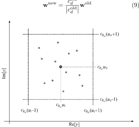
(8) wherey(k) =yR(k)+jyI(k). Fig. 1 depicts the decision

boundaries associated with the decision ˆb_d(k) =b_l,q. In general,wH_p

d is complex-valued and the rotating

op-eration

wnew= c

old

d

cold

d

wold (9)

Fig. 1 Generic decision boundaries associated with point

cdbl,q assumingcId= 0, and illustrations of symmetric

distribution ofYl,q around the mass centercdbl,q

can be used to makecdreal and positive. This rotation

at the receiver in order to make a decision regarding the transmitted symbolb_d(k).

The classical design for the linear filter (1) is based on minimizing the MSE term of E[|bd(k)−y(k)|2],

which leads to the following MMSE solution

w_MMSE=

PPH+2σ

2

n

σ2

b

I_L

−1

p_d (10)

where σ2

b = E[|bi(k)|2]. The MMSE solution

gener-ally does not provide a minimum error probability, un-less the conditional p.d.f. of y(k) givenb_d(k) =b_l,q is Gaussian. However, the p.d.f. ofy(k) is obviously non-Gaussian, as can be seen from (5). Since the SER is the true performance indicator, it is desireable to consider the optimal MSER filter solution.

3

Minimum symbol error rate solution

Denote theNb=MN number of possible sequences

of b(k) as b_i, 1 i N_b. Then ¯x(k) can only take values from the finite signal set defined by

X {x¯_i=Pb_i, 1iN_b}. (11)

This set can be partitioned intoM subsets, depending on the specific value ofb_d(k), as follows:

Xl,q{¯xi∈ X : bd(k) =bl,q}, 1l, q √

M . (12)

Recall that the filter’s output is given by

y(k) =wH¯x(k) +wHn(k) = ¯y(k) +e(k) (13)

wheree(k) is Gaussian distributed with zero mean and

E[|e(k)|2] = 2σ_n2wHw. The noise-free part of the fil-ter’s output, namely ¯y(k), only takes values from the scalar set

Y {y¯i=wHx¯i, 1iNb} (14)

and Y can be divided into the M subsets conditioned on the value ofbd(k):

Yl,q{y¯i∈ Y : bd(k) =bl,q}, 1l, q √

M . (15)

Lemma 1. The subsetsX_l,q, 1l, q √M, sat-isfy the shifting properties:

Xl+1,q=Xl,q+ 2pd, 1l √

M −1 (16)

Xl,q+1=Xl,q+j2pd, 1q √

M−1 (17)

Xl+1,q+1 =Xl,q+ (2 +j2)pd, 1l, q √

M−1. (18)

Proof. From the definitions ofPandb_i, for each ¯

x_i(l,q)∈ X_l,q, there exists a ¯x_i(l+1,q)∈ X_l+1,q, such that

¯

x(_il+1,q)= ¯x(_il,q)+ (bl+1,q−bl,q)pd= ¯x(il,q)+ 2pd. (19)

This verifies the shifting property (16). The proofs for

(17) and (18) are similar.

Lemma 2. As a direct consequence of Lemma 1, the subsets Yl,q, 1 l, q

√

M, satisfy the shifting properties:

Yl+1,q =Yl,q+ 2cd, 1l √

M−1 (20)

Yl,q+1=Yl,q+j2cd, 1q √

M −1 (21)

Yl+1,q+1=Yl,q+ (2 +j2)cd, 1l, q √

M−1. (22)

Lemma 3. The points ofYl,q are distributed

sym-metrically around the symbol pointcdbl,q.

Lemma 3 is obvious and is a direct consequence of symmetric distribution of the symbol constellation (3). This symmetric property is also illustrated in Fig. 1. Note that the distribution ofY_l,q is symmetric with re-spect to the two vertical decision boundariescRd(ul±1)

and with respect to the two horizontal decision bound-ariesc_Rd(u_q±1).

For a linear filter to perform adequately it is implic-itly assumed that the system is linearly separable. Lin-ear separability is interpreted as follows: there exists w satisfying condition (6) such thatYl,q is completely

separated from Y_l+1,q by the line c_Rd(u_l + 1) +ju, for 1 l √M − 1 and 1 q √M, and Yl,q is completely separated from Yl,q+1 by the line u+jc_Rd(u_q+ 1), for 1l√M and 1q√M−1, where u ∈ (−∞, ∞) denotes a real-valued variable. Linear separability is not always guaranteed in prac-tice. When the underlying system is linearly insepa-rable, a linear filter will have an irreducibly high SER floor and nonlinear filtering is required to achieve ade-quate performance[25∼31]_.

3.1

Symbol error rate expression

For the linear filter with weight vectorw satisfying (6), denote

P_E(w) = Prob{ˆb_d(k)=b_d(k)} (23)

PER(w) = Prob{ˆbRd(k)=bRd(k)} (24)

PEI(w) = Prob{ˆbId(k)=bId(k)}. (25)

It is then easy to see that the SER is given by

PE(w) =PER(w) +PEI(w)−PER(w)PEI(w). (26)

The conditional p.d.f. of y(k) given b_d(k) = b_l,q is a Gaussian mixture defined by

p(y|bl,q) =

1

Nsb2πσ2nwHw Nsb

i=1 e−

|y−y¯(_il,q)|2

2σ_n2wHw ₍₂₇₎

where Nsb = Nb/M is the number of points in Yl,q,

¯

Note that cd is real and the symbol decision is

decoupled into (7) and (8). Taking into account the symmetric distribution of Yl,q, see Lemma 3, for

2 l √M −1, the conditional error probability of ˆ_b

Rd(k)=ulgiven bRd(k) =ul is

P_ER,l(w) = 1

Nsb2πσn2wHw Nsb

i=1 ∞

−∞e −(yI−y¯

(l,q)

Ii )2

2σ_n2wHw _{d y}

I×

c_Rd(ul−1)

−∞

+

∞

c_Rd(ul+1)

e−

(yR−y¯(l,q)

Ri )2

2σ2_nwHw _dy

R= 2 Nsb Nsb i=1

Q(g_Ri(l,q)(w)) (28)

where

Q(u) =√1 2π

∞

u

e−z22_{dz (29)}

g(_Ril,q)(w) = y¯

(l,q)

Ri −cRd(ul−1)

σn √

wH_w . (30)

Further taking into account the shifting property, see Lemma 2 and noting that the error only occurs at one size in (28) if l = 1 or √M, it is straightforward to show that

P_ER(w) = √

M−1 √ M 2 Nsb Nsb i=1

Q(g(_Ril,q)(w)) =

γ 1 N_sb

Nsb

i=1

Q(g_Ri(l,q)(w)) (31)

whereγ= 2 √

M−2 √

M . It is seen thatPER can be

eval-uated using the real part of any single subsetYl,q.

Similarly,P_EI can be evaluated using the imaginary part of any single subsetY_l,q as

PEI(w) =γ

1

N_sb

Nsb

i=1

Q(g_Ii(l,q)(w)) (32)

with

g(_Iil,q)(w) = y¯

(l,q)

Ii −cRd(uq−1)

σ_n√wH_w . (33)

3.2

Minimum symbol-error-rate solution

The MSER solutionw_MSERin principle is obtained by minimizing PE(w) with respect to w. However,

there is no simple way of doing so due to the cross coupled termPER(w)PEI(w). Instead, the MSER

so-lution is defined as the one that minimizes the upper bound of the SER given by

PEB(w) =PER(w) +PEI(w). (34)

That is,

w_MSER= arg min

w PEB(w). (35)

The upper bound P_EB(w) is very tight, i.e. very close to the true SERPE(w). Unlike the closed-form MMSE

solution (10), a numerical optimization has to be ap-plied to obtain an MSER solutionw_MSER. The gradi-ents ofPER(w) andPEI(w) with respect tow can be

shown to be respectively

∇PER(w) =

γ

2Nsb √

2πσn √

wH_w

Nsb i=1 e− ¯

y(l,q)

Ri −cRd(ul−1)

2 2σ2_nwHw

×

¯

y(_Ril,q)−cRd(ul−1)

wH_w w−x¯ (l,q)

i + (ul−1)pd

(36)

∇PEI(w) =

γ

2N_sb√2πσ_n√wH_w

Nsb i=1 e− ¯

y(l,q)

Ii −cRd(uq−1)

2 2σ2_nwHw

×

¯

y_Ii(l,q)−c_Rd(u_q−1) wH_w w+jx¯

(l,q)

i + (uq−1)pd

.

(37)

With the gradient∇PEB(w) =∇PER(w) +∇PEI(w),

the optimization problem (35) can be solved for iter-atively using a gradient-based optimization algorithm. Since the SER is invariant to a positive scaling of w, it is computationally advantageous to normalize w to a unit-length using

w:=w/√wH_{w (38)}

after every iteration, so that the gradients (36) and (37) can be simplified to:

∇PER(w) =

γ

2Nsb √

2πσn Nsb i=1 e− ¯

y(l,q)

Ri −cRd(ul−1)

2 2σ2_n ×

¯

y(_Ril,q)−cRd(ul−1)

w−x¯(_il,q)+ (ul−1)pd

(39)

∇P_EI(w) = γ 2N_sb√2πσ_n

Nsb i=1 e− ¯

y(l,q)

Ii −cRd(uq−1)

2 2σ_n2 ×

¯

y(_Iil,q)−cRd(uq−1)

w+jx¯(_il,q)+ (uq−1)pd

.

(40)

The rotating operation (9) should also be applied af-ter each iaf-teration to ensure a real and positive cd. A

further saving in computation is achieved by choos-ing the subset with l, q = 1 +√M /2, giving rise to

ul−1 =uq−1 = 0. We point out that the simplified

conjugate gradient algorithm[15,32]_{provides an efficient}

4

Adaptive MSER filtering

To derive an adaptive version of the MSER filter-ing, it is more convenient to explicitly write down the p.d.f. ofy(k)

p(y) = 1

N_b2πσ2

nwHw

√ M l=1 √ M q=1 Nsb i=1 e−

|y−y¯(l,q)

i |2

2σ2_nwHw ₍₄₁₎

and to express the two error probabilities alternatively as

PER(w) =

γ Nb √ M l=1 √ M q=1 Nsb i=1

Q(g(_Ril,q)(w)) (42)

P_EI(w) = γ

N_b √ M l=1 √ M q=1 Nsb i=1

Q(g_Ii(l,q)(w)). (43)

In reality, the p.d.f. of y(k) is unknown. Parzen window or kernel density estimate[21−23] _{is a well}

known method for estimating a probability distribu-tion. Parzen window method estimates a p.d.f. using a window or block ofy(k) by placing a symmetric uni-modal kernel function on each y(k). Kernel density estimation is capable of producing reliable p.d.f. es-timates with short data records and is natural when dealing with Gaussian mixtures, such as the one given in (41). In our application, it is obvious and natural to choose a Gaussian kernel function with a kernel width

ρn √

wH_{wthat is similar in form to the noise standard}

deviationσn √

wH_w.

4.1

Block-data gradient adaptive MSER

algorithm

Given a block of K training samples {x(k), bd(k)}Kk=1, a kernel density estimate of the p.d.f.

(41) is readily given by

ˆ

p(y) = 1

K2πρ2

nwHw K

k=1 e−

|y−y(k)|2

2ρ2_nwHw ₍₄₄₎

where the scaling parameterρ_n is related to the stan-dard deviationσn of the system noise. In [22], a lower

bound ofρn =

₄

3K

1 5_σ

n is suggested. In practice,ρn

can often be chosen from a large range of values. From this estimated p.d.f. (44), the estimated upper-bound SER expression is given by

ˆ

PEB(w) = ˆPER(w) + ˆPEI(w) =

γ K

K

k=1

(Q(ˆgRk(w)) +Q(ˆgIk(w)))

(45)

with ˆ

gRk(w) =

yR(k)−ˆcRd(bRd(k)−1)

ρn √

wH_w (46)

ˆ

gIk(w) =

yI(k)−cˆRd(bId(k)−1)

ρn √

wH_w (47)

where ˆcRd= Re[wHpˆd] and ˆpdan estimate ofpd. The

gradient of ˆPEB(w) can readily be calculated with

∇_Pˆ_{ER(w) =} γ 2K√2πρn

√ wH_w

K

i=1 e−

(yR(k)−ˆcR_d(bR_d(k)−1)₎2 2ρ2_nwHw

×

yR(k)−ˆcRd(bRd(k)−1)

wH_w w−x(k)+(bRd(k)−1)ˆpd

(48)

∇_Pˆ_{EI(w) =} γ

2K√2πρ_n√wH_w

K

i=1 e−

(yI(k)−ˆcR_d(bI_d(k)−1)₎2 2ρ2_nwHw

×

y_I(k)−ˆc_Rd(b_Id(k)−1)

wH_w w+jx(k)+(bId(k)−1)ˆpd

(49)

Upon substituting ∇PEB(w) by ∇PˆEB(w) = ∇_Pˆ_ER(w)+∇Pˆ_{EI(w) in the simplified conjugate} gradi-ent updating mechanism, a block-data based adaptive algorithm is obtained. The step sizeµof the conjugate gradient algorithm and the scaling parameter ρ_n are two algorithmic parameters, which control the rate of convergence and determine the accuracy of the p.d.f. and hence SER estimate.

4.2

Stochastic gradient adaptive MSER

algorithm

In the Parzen window estimate (44), the kernel widthρ_n√wH_{wdepends on the filter weight vectorw.}

In a general density estimate, there is no reason why the width parameter should be chosen in such a way except that the dependency of the width parameter to w in the true density (41) is noticed. However, the SER is invariant to wHw. To fully take advantage of this fact, it is proposed to used a constant width ρ_n

in density estimates. One advantage of using a con-stant width ρn, rather than a variable one ρn

√ wH_w,

in the density estimate is that the gradient of the re-sulting estimated SER has a much simpler form, which leads to considerable reduction in computational com-plexity. This is particularly relevant to the derivation of stochastic gradient updating mechanisms. Adopting this approach, an alternative Parzen window estimate of the true p.d.f. (41) is given by

˜

p(y) = 1

K2πρ2

n K

k=1 e−

|y−y(k)|2

2ρ2_{n (50)}

and an approximation of the upper-bound SER is

˜

γ K

K

k=1

(Q(˜gRk(w)) +Q(˜gIk(w)))

(51)

with ˜

gRk(w) =

yR(k)−ˆcRd(bRd(k)−1)

ρn

(52)

˜

gIk(w) =

yI(k)−ˆcRd(bId(k)−1)

ρ_n . (53)

This approximation is valid, provided that the width

ρn is chosen appropriately.

To derive a sample-by-sample adaptive algorithm, consider a single-sample “estimate” ofp(y), namely

˜

p(y, k) = 1 2πρ2

n

e−

|y−y(k)|2

2ρ2_{n (54)}

and the corresponding one-sample SER “estimate” ˜

P_EB(w, k). Using the instantaneous stochastic gradi-ent of∇P˜EB(w, k) =∇P˜ER(w, k) +∇P˜EI(w, k) with

∇_P˜_{ER(w, k) =} γ 2√2πρn

e−

(yR(k)−ˆcR_d(k)(bR_d(k)−1)₎2 2ρ2_n ×

(−x(k) + (bRd(k)−1)ˆpd) (55)

∇_P˜_{EI(w, k) =} γ 2√2πρn

e−

(yI(k)−ˆcR_d(k)(bI_d(k)−1))2

2ρ2_n ×

(jx(k) + (bId(k)−1)ˆpd) (56)

gives rise to a stochastic gradient adaptive algorithm, referred to as the LSER algorithm:

w(k+ 1) =w(k) +µ

−∇_P˜_{EB(w(k), k) (57)}

ˆ

cd(k+ 1) =wH(k+ 1)ˆpd (58)

w(k+ 1) = ˆcd(k+ 1) |ˆcd(k+ 1)|

w(k+ 1) (59)

where the adaptive gain µ and the kernel width ρn

should be set appropriately to ensure an adequate per-formance in terms of convergence rate and steady-state SER misadjustment. Note that there is no need to normalize the weight vector to a unit-length after each update.

It is interesting to see some analogy between the traditional adaptive filtering approach based on the MMSE criterion and the proposed adaptive MSER fil-tering approach. The second-order statistics required to compute the Wiener solution can be estimated using a block of samples, and by considering a single-sample estimate, a stochastic gradient adaptive MMSE algo-rithm, namely the LMS, is derived. The p.d.f. required to determine the MSER solution can be approximated

with a kernel density estimate based on a block of sam-ples, and by considering a single-sample density esti-mate, a stochastic gradient adaptive MSER algorithm is formulated.

5

Application examples

The effectiveness of the proposed adaptive MSER filtering approach is demonstrated using two applica-tions.

5.1

Single-user channel equalization

In the communication system involving a dispersive channel, the received signal sample can be expressed as[20]

r(k) =

na−1

i=0

a_ib(k−i) +n(k) (60)

wherenais the channel impulse response (CIR) length,

aiare complex-valued channel taps,{b(k)}is the

trans-mitted data symbol sequence, and n(k) a complex-valued additive white Gaussian noise withE[|n(k)|2_{] =}

2σ_n2. The system signal to noise ratio (SNR) is defined as SNR =aH_aσ2

b/2σn2, where a= [a0 a1· · ·ana−1]T is

the channel tap vector andE[|b(k)|2_{] =σ}2

b. A decision

feedback equalizer (DFE) is employed at the receiver, which takes the form

y(k) =wHr(k) +fHbˆ_{f b}(k) (61)

where r(k) = [r(k) r(k − 1)· · ·r(k − L + 1)]T _is

the observation vector, ˆb_{f b}(k) = [ˆb(k − d− 1)· · · ˆ

b(k−d−nf b)]T is the past detected symbol vector,

w and f = [f₁· · ·f_{nf b}]T _{are the feedforward and}

feed-back filter coefficient vectors with orders L and nf b

respectively. At symbol instancek, the DFE provides an estimate ˆb(k−d) of the transmitted symbolb(k−d), wheredis called the decision delay. The DFE structure parameters will be chosen as

L=n_a, n_{f b}=n_a−1, d=n_a−1 (62)

as this choice is sufficient to guarantee a desired linear separability, see Lemma 4.

The DFE (61) can be translated into the linear fil-ter (1) under the assumption that the past decisions are correct (also see [6]). The received signal vector can be expressed as

r(k) = ¯r(k) +n(k) =Ab(k) +n(k) (63)

where theL×(L+na−1) CIR matrixAhas the form

A=

⎡ ⎢ ⎢ ⎢ ⎢ ⎣

a0 a1 · · · ana−1 0 · · · 0

0 a0 a1 · · · ana−1 . .. ...

..

. . .. . .. . .. _{· · ·} . .. 0 0 · · · 0 a0 a1 · · · ana−1

[P|P_{f b}] (64)

withPhaving a dimension ofL×LandP_{f b} having a dimension ofL×(na−1), and

b(k) = [b(k)b(k−1)· · ·b(k−d)|

b(k−d−1)· · ·b(k−L−na+ 2)]T=

[bT_{f f}(k)|bT_{f b}(k)]T. (65)

Noticing (62), the last column of P is p_d = [ana−1· · ·a1 a0]T. Under the assumption that the past

decisions are correct, ˆb_{f b}(k) =b_{f b}(k) andr(k) can be expressed as

r(k) =Pb_{f f}(k) +P_{f b}bˆ_{f b}(k) +n(k). (66)

Thus, the decision feedback translates the original ob-servation spacer(k) into a new spacex(k) defined by

x(k)r(k)−P_{f b}bˆ_{f b}(k) =Pb_{f f}(k) +n(k) = ¯

x(k) +n(k). (67)

In this translated observation space, the DFE (61) be-comes

y(k) =wHx(k) = ¯y(k) +e(k). (68)

The feedback filter coefficients do not disappear. They have been set to their optimal values f_opt = −PH_{f b}w_MMSE, where w_MMSE denotes the MMSE so-lution for w. There is no need to explicitly estimate f_opt, because the elements of x(k) can be computed recursively according to [6] as

⎧ ⎨ ⎩

x(k−i) =z−1_{x(k−i+ 1)−a}

na−iˆb(k−d−1),

i=L−1,· · ·,2,1

x(k) =r(k)

(69) where z−1 _{denotes the unit delay operator. Thus, in}

an adaptive implementation, one needs to estimate the CIR using for example the LMS algorithm, rather than estimatef. Note that the CIR is needed anyway in or-der to make the symbol decision according to (7) and (8).

The equalizer (68) and its observation model (67) have identical forms to the linear filter (1) and its ob-servation model (2), with N =L =na. Furthermore,

the DFE has the following desired property of linear separability.

Lemma 4.With the choice of DFE structure (62), Yl,q, 1l, q

√

M, are linearly separable.

Proof. Choose the weight vector w = [0 0· · ·0 1

a∗₀]T. It is obvious that condition (6) is

sat-isfied, as wHp_d = 1. For l = 1,· · ·,√M −1 and 1q√M, it is easy to see that

wHx¯(_il,q)=bl,q, ∀x¯(il,q)∈ Xl,q (70)

wHx¯(_il+1,q)=b_l+1,q, ∀x¯(_il+1,q)∈ X_l+1,q. (71)

That is, Yl,q is completely separated from Yl+1,q by

the line (u_l+ 1) +ju. Similarly, for 1l √M and

q = 1,· · ·,√M −1, Yl,q is completely separated from Yl,q+1 by the lineu+j(uq+ 1).

In the simulation, the 16-QAM symbols were trans-mitted through the two-tap channelaT_{= [0.2−j0.2 −}

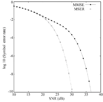
1.0 +j1.0]. The DFE structure parameters were set ac-cording to (62) as L = 2, d = 1 and nf b = 1. Fig. 2

compares the SER performance of the MMSE DFE with

Fig. 2 Symbol error rate performance comparison of the MMSE and MSER DFEs

that of the MSER one, where it can be seen that the MSER solution offers more than 5 dB improvement in SNR at the SER level of 10−4 _{over the MMSE}

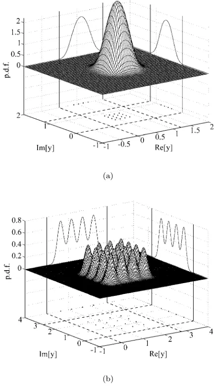
solu-tion. The conditional p.d.f. p(y|bl,q), the two marginal

conditional p.d.f’.sp(yR|bl,q) andp(yI|bl,q), the subset Yl,q and its real and imaginary parts of the MMSE

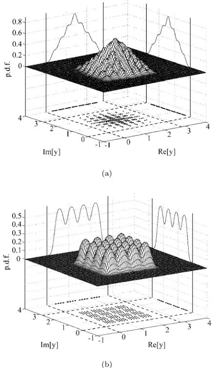
DFE output, givenb(k−d) = 1 +j and with an SNR = 27 dB, are compared with those of the MSER DFE in Fig. 3. For this example, the total number of signal points is N_b = 162 _{= 256 and therefore Y}

l,q contains

Nsb= 16 points. In Fig. 3, the equalizer weight vector

w has been normalized to a unit length, so that the SER is determined by the minimum distance from the subset Yl,q to the corresponding decision boundaries.

this density distribution is evident for the MSER DFE.

(a)

(b)

Fig. 3 Conditional probability density functions

p(y|+ 1 +j) (surfaces), marginal conditional probability density functionsp(yR|+ 1 +j) andp(yI|+ 1 +j) (curves), signal subsetsY3,3 (dots) and their real and

imaginary parts (dots) for: (a) the MMSE DFE, and (b) the MSER DFE, given SNR = 27 dB. The equalizer

weight vector has been normalized to a unit length

The performance of the block-data based adaptive MSER algorithm with the simplified conjugate gradi-ent updating mechanism was next studied. A perfect estimate ˆp_d was assumed and the step sizeµ and the kernel widthρnwere determined empirically to provide

the best performance in terms of convergence speed and estimation accuracy. Fig. 4 illustrates the convergence rate of the algorithm under SNR = 27 dB and given two different initial weight vector conditions, where two block sizesK= 50 and 100 were used. From Fig. 4, it can be seen that the convergence speed of this block-data adaptive MSER algorithm is rapid. As the SER estimate ˆPEB(w) is a complicated nonlinear function

of w, the initial condition affects convergence speed. For this example, with w(0) chosen arbitrarily to be [0.0 +j0.0 0.1−j0.1]T_{, it took only one iteration to}

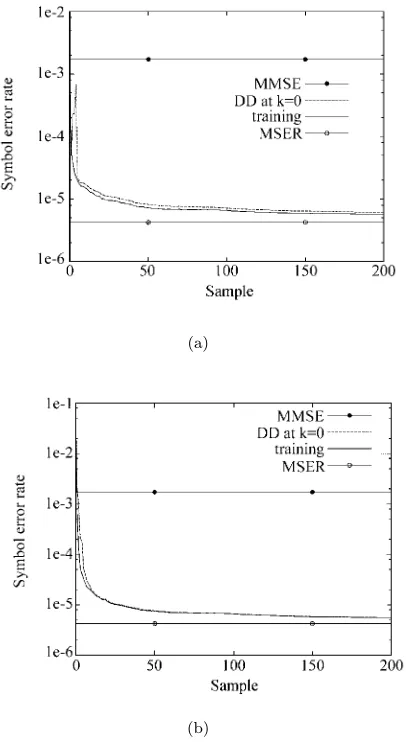
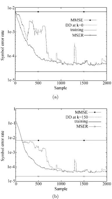
converge, compared this with about 40 iterations that was needed with w(0) = w_MMSE. The performance of the stochastic gradient adaptive MSER algorithm was then investigated. Fig. 5 shows the learning curves of the LSER algorithm averaged over 100 runs, given SNR = 27 dB and two different initial weight vector conditions. From Fig. 5, it can be seen that this LSER algorithm has a fast convergence rate. There are two learning curves in both Fig. 5 (a) and (b), correspond-ing to traincorrespond-ing and decision directed (DD) adaptation in whichb(k−d) is substituted by the equalizer’s esti-mate ˆb(k−d). It is seen that even with the DD adap-tation, the LSER algorithm performs well.

(a)

(b)

Fig. 4 Convergence rate of the block-data gradient adaptive MSER algorithm for the equalization example

given SNR = 27 dB: (a)w(0) =wMMSE,µ= 0.8 and

(a)

(b)

Fig. 5 Learning curves of the stochastic gradient adaptive MSER algorithm averaged over 100 runs for the

equalization example given SNR = 27 dB: (a)

w(0) =wMMSE,µ= 0.9 andρ2n= 50σn2 ≈1.04, and (b) w(0) = [0.0 +j0.0 0.1−j0.1]T,µ= 0.9 and

ρ2n= 100σ2n≈2.08, where DD denotes decision directed

adaptation with ˆb(k−d) substitutingb(k−d)

5.2

Adaptive beamforming assisted

re-ceiver

The ever-increasing demand for mobile communica-tion capacity has motivated the employment of space division multiple access for improving the achievable spectral efficiency. A particular approach that has shown real promise in achieving substantial capacity enhancements is the use of adaptive beamforming with antenna arrays. Adaptive beamforming is capable of separating signals transmitted on the same carrier fre-quency, provided that they are separated sufficiently in the spatial domain. Consider the system that supports

N users (sources) which transmit on the same carrier frequency ω = 2πf, and assume that the channel is

narrow-band which does not induce intersymbol inter-ference. The linear antenna array considered consists of

L uniformly spaced elements, and the signals received by the L-element antenna array can be expressed in the form of (2), where the L×N system matrix Pis defined by

P= [A0s0A1s1· · ·AN−1sN−1] (72)

withAi denoting the channel coefficient for useriand

the steering vector for sourcei

s_i= [exp(jωt0(θi))· · ·exp(jωtL−1(θi))]T (73)

with tl(θi) being the relative time delay at array

el-ement l for source i and θ_i the direction of arrival for source i. The transmitted user symbol vector is b(k) = [b0(k)b1(k)· · ·bN−1(k)]T. Without any loss of

generality, source 0 is assumed to be the desired user and the rest of the sources are the interfering users. The desired user’s SNR is defined as SNR = |A0|2σb2/2σn2

and the desired signal to interference ratio (SIR) with respect to interfering useriis defined as SIRi=A20/A2i

for 1 i N−1. The beamformer at receiver is a linear filter in the form of (1) withd= 0 in the decision rule (7) and (8).

The simulation example consisted of three 16-QAM signal sources and a two-element antenna array. Fig. 6 shows the locations of the desired source and the inter-fering sources. The minimum spatial separation was the difference in angles of arrival between the desired user 0 and the interferer 2, which wasθ 70◦. Fig. 7 compares the SER of the MMSE solution with that of the MSER one, given θ= 60◦ and under two different conditions: (a) the desired user and the two interfering sources had equal power, and (b) the desired user and

Fig. 6 Locations of the desired source and the interfering sources with respect to the two-element linear antenna

the interfering source 1 had equal power, but the in-terfering source 2 had 6 dB higher power than the de-sired user. It can be seen that when the 2nd interfering user’s power was increased by 6 dB, the MMSE beam-former’s performance degraded considerably while the performance of the MSER beamformer was only af-fected slightly. Thus, the MSER beamformer is robust to the near-far effect. Figs. 8 and 9 depict the condi-tional p.d.f. p(y|1 +j), the two marginal conditional p.d.f.’sp(yR|1 +j) andp(yI|1 +j), the subsetY3,3and

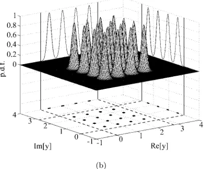
its real and imaginary parts for the MMSE and MSER beamformers, given θ = 60◦, SNR = 27 dB, and two SIR conditions, respectively. The total number of sig-nal points was Nb = 163 = 4096 and the subset Y3,3

containedNsb= 256 points. It is seen from Fig. 8 that

in the equal user power case, the minimum distance from Y3,3 to its corresponding decision boundaries for

the MSER solution was slightly larger than that for the MMSE solution. This explains the slightly better SER performance of the MSER beamformer over the MMSE one as shown in Fig. 7 with SIR1= SIR2= 0 dB. When

facing a strong interference signal, Fig. 9 (a) shows that the minimum separation between Yl,q for the MMSE

solution was reduced dramatically, thus causing a sig-nificant performance degradation as seen in Fig. 7 for the case of SIR2 =−6 dB. The reason of near-far

ro-bustness for the MSER solution can be seen clearly from Fig. 9 (b), which shows an almost unchanged min-imum separation betweenYl,qcompared with the equal

user power case.

Fig. 7 Symbol error rate performance comparison of the MMSE and MSER beamformers, givenθ= 60◦,

SIR1= 0 dB, and two SIR2 (0 dB and -6 dB)

(a)

(b)

Fig. 8 Conditional probability density functions

p(y|+ 1 +j) (surfaces), marginal conditional probability density functionsp(yR|+ 1 +j) andp(yI|+ 1 +j) (curves), signal subsetsY3,3 (dots) and their real and

imaginary parts (dots) for: (a) the MMSE beamformer, and (b) the MSER beamformer, givenθ= 60◦, SNR = 27 dB and SIR₁= SIR₂= 0 dB. The beamformer weight vector has been normalized to a unit length

(b)

Fig. 9 Conditional probability density functions

p(y|+ 1 +j) (surfaces), marginal conditional probability density functionsp(yR|+ 1 +j) andp(yI|+ 1 +j) (curves),

signal subsetsY₃,3 (dots) and their real and imaginary parts (dots) for: (a) the MMSE beamformer, and (b) the

MSER beamformer, givenθ= 60◦, SNR = 27 dB, SIR1= 0 dB and SIR2=−6 dB. The beamformer weight

vector has been normalized to a unit length

The performance of the two beamformers was also investigated under the equal user power condition. The varying minimum spatial separationθ, and the results are depicted in Fig. 10. Forθ= 70◦, the performances of the two beamformers were indistinguishable. When

θ was reduced to 60◦ and 58◦, the MSER beamformer achieved above 1 dB and 3 dB improvements in SNR, respectively, at the SER level of 10−4over the MMSE solution. For θ = 55◦, the MMSE beamformer could not achieve linear separability and exhibited an irre-ducible SER floor, while the MSER beamformer could still manage to achieve a linear separability. When the minimum spatial separation was below 55◦, the system was inherently linearly inseparable.

Performance of the block-data gradient adaptive MSER algorithm was next tested. Again a perfect esti-mate ˆp_d was assumed and the step sizeµand the ker-nel widthρnwere found empirically to provide the best

performance in terms of convergence speed and estima-tion accuracy. Fig. 11 illustrates the convergence rates of the algorithm given SNR = 27 dB, SIR₁= 0 dB and SIR2=−6 dB, and with the two different initial weight

vectors. It can be seen that this block-data adaptive MSER algorithm converges rapidly. Performance of the stochastic gradient adaptive MSER algorithm was also investigated. Fig. 12 shows the learning curves of the algorithm averaged over 100 runs, under the same con-ditions of Fig. 11, where DD denotes decision-directed adaptation with ˆb0(k) substitutingb0(k) as the desired

response. It can be seen that once the SER is below certain level (0.01 for this example), DD adaptation

can be applied.

(a)

(b)

Fig. 10 Symbol error rate performance comparison of the MMSE and MSER beamformers given SIR₁= SIR2= 0 dB: (a)θ= 70◦and 60◦, and (b)θ= 58◦and 55◦

(b)

Fig. 11 Convergence rate of the block-data gradient adaptive MSER algorithm for the beamforming example

given SNR = 27 dB, SIR1= 0 dB and SIR2=−6 dB: (a)w(0) =wMMSE,µ= 0.05 andρ2n=σn2 ≈0.01,

and (b)w(0) = [0.7−j0.1 0.6 +j0.1]T,

µ= 0.05 andρ2n=σn2 ≈0.01

(a)

(b)

Fig. 12 Learning curves of the stochastic gradient adaptive MSER algorithm averaged over 100 runs for the

beamforming example given SNR = 27 dB, SIR1= 0 dB and SIR₂=−6 dB: (a)w(0) =wMMSE,µ= 0.0005 and

ρ2n=σn2 ≈0.01, and (b)w(0) = [0.7−j0.1 0.6 +j0.1]T, µ= 0.0005 andρ2n=σn2 ≈0.01, where DD denotes

decision directed adaptation with ˆb0(k) substitutingb0(k)

6

Conclusions

An adaptive linear filtering technique based on the novel MSER principle has been proposed for applica-tions to communication systems with complex-valued filters and M-QAM signalling. It has been demon-strated that the MSER filtering is capable of achieving significant performance gains in terms of reduced SER over the traditional MMSE filtering. This is due to the fact that the MSER filtering can exploit effectively the non-Gaussian nature of the underlying system density distribution. Adaptive implementation of the proposed MSER filtering has been developed based on the Parzen window estimation for the p.d.f. of the filter’s out-put. A block-data based simplified conjugate gradient adaptive MSER algorithm has been shown to converge rapidly and requires a reasonably small data block size to accurately approximate the theoretical MSER solu-tion. An LMS-style stochastic gradient adaptive MSER algorithm, referred to as the LSER, has been shown to perform well, and the algorithm has similar computa-tional requirements to the low-complexity LMS algo-rithm.

References

[1] B. Widrow, S. D. Stearns. Adaptive Signal Processing. Prentice-Hall, Englewood Cliffs, NJ, 1985.

[2] S. Haykin. Adaptive Filter Theory. 3rd edition, Prentice-Hall, Upper Saddle River, NJ, 1996.

[3] E. Shamash, K. Yao. On the Structure and Performance of a Linear Decision Feedback Equalizer Based on the Minimum Error Probability Criterion. InProceedings of International Communications Conference, pp. 25F1−25F5, 1974. [4] S. Chen, E. S. Chng, B. Mulgrew, G. Gibson.

Minimum-BER Linear-combiner DFE. InProceedings of International Communications Conference, Dallas, Texas, vol. 2, pp. 1173−1177, 1996.

[5] C. C. Yeh, J. R. Barry. Approximate Minimum Bit-Error Rate Equalization for Binary Signaling. InProceedings of In-ternational Communications Conference, Montreal, Canada, vol. 2, pp. 1095−1099, 1997.

[6] S. Chen, B. Mulgrew, E. S. Chng, G. Gibson. Space Trans-lation Properties and the Minimum-BER Linear-combiner DFE.IEE Proceedings of Communications, vol. 145, no. 5, pp. 316−322. 1998.

[7] B. Mulgrew, S. Chen. Stochastic Gradient Minimum-BER Decision Feedback Equalisers. InProceedings of IEEE Sym-posium on Adaptive Systems for Signal Processing, Commu-nication and Control, Lake Louise, Alberta, Canada, Oct. 1-4, pp. 93−98, 2000.

[8] C. C. Yeh, J. R. Barry. Adaptive Minimum Bit-Error Rate Equalization for Binary Signaling. IEEE Transactions Com-munications, vol. 48, no. 7, pp. 1226−1235, 2000.

[9] B. Mulgrew, S. Chen. Adaptive Minimum-BER Decision Feedback Equalisers for Binary Signalling. Signal Process-ing, vol. 81, no. 7, pp. 1479−1489, 2001.

[11] C. C. Yeh, R. R. Lopes, J. R. Barry. Approximate Mini-mum Bit-Error Rate Multiuser Detection. InProceedings of Globecom’98, Sydney, Australia, pp. 3590−3595, 1998. [12] X. F. Wang, W. S. Lu, A. Antoniou. Constrained

Minimum-BER Multiuser Detection. InProceedings of International Conference on Acoustics Speech and Signal Processing, Phoenix, USA, vol. 5, pp. 2603−2606, May 14-18, 1999. [13] I. N. Psaromiligkos, S. N. Batalama, D. A. Pados. On

Adap-tive Minimum Probability of Error Linear Filter Receivers for DS-CDMA Channels. IEEE Transactions Communications, vol. 47, no. 7, pp. 1092−1102, 1999.

[14] S. Chen, A. K. Samingan, B. Mulgrew, L. Hanzo. Adap-tive Minimum-BER Linear Multiuser Detection. In Proceed-ings of International Conference on Acoustics Speech and Signal Processing. Salt Lake City, Utah, USA, vol.4, pp. 2253−2256, May 7-11, 2001.

[15] S. Chen, A. K. Samingan, B. Mulgrew, L. Hanzo. Adaptive Minimum-BER Linear Multiuser Detection for DS-CDMA Signals in Multipath Channels. IEEE Transactions on Sig-nal Processing, vol. 49, no. 6, 1240−1247, 2001.

[16] R. C. de Lamare, R. Sampaio-Neto. Adaptive MBER De-cision Feedback Multiuser Receivers in Frequency Selective Fading Channels.IEEE Communications Letters, vol. 7, no. 2, pp. 73−75, 2003.

[17] S. Chen, N. N. Ahmad, L. Hanzo. Smart Beamforming for Wireless Communications: A Novel Minimum Bit-error Rate Approach. InProceedings of 2nd IMA International Confer-ence Mathematics in Communications, Lancaster, U.K., Dec. 16-18, 2002.

[18] S. Chen, L. Hanzo, N. N. Ahmad. Adaptive Minimum Bit-error Rate Beamforming Assisted Receiver for Wireless Com-munications. InProceedings of International Conference on Acoustics Speech and Signal Processing 2003, Hong Kong, China, vol. IV, pp. 640−643, April 6-10, 2003.

[19] S. Chen, N. N. Ahmad, L. Hanzo. Adaptive Minimum Bit-Error Rate Beamforming. IEEE Transactions on Wireless Communications, vol. 4, no. 2, pp. 341−348, 2005. [20] J. G. Proakis. Digital Communications. 3rd ed.,

McGraw-Hill, New York, 1995.

[21] E. Parzen. On Estimation of a Probability Density Function and Mode. The Annals of Mathematical Statistics, vol. 33, pp. 1066−1076, 1962.

[22] B. W. Silverman. Density Estimation. Chapman Hall, Lon-don, 1996.

[23] A. W. Bowman, A. Azzalini. Applied Smoothing Techniques for Data Analysis. Oxford University Press, Oxford, UK, 1997.

[24] R. Johnson, Jr. P. Schniter, T. J. Endres, J. D. Behm, D. R. Brown, R. A. Casas. Blind Equalization Using the Constant Modulus Criterion: A Review. Proceedings of IEEE, vol.

86, no. 10, pp. 1927−1950, 1998.

[25] S. Chen, B. Mulgrew, P. M. Grant. A Clustering Technique for Digital Communications Channel Equalisation Using Ra-dial Basis Function Networks. IEEE Transactions on Neural Networks, vol. 4, no. 4, pp. 570−579, 1993.

[26] S. Chen, B. Mulgrew, S. McLaughlin. Adaptive Bayesian Equaliser with Decision Feedback. IEEE Transactions on Signal Processing, vol. 41, no. 9, pp. 2918−2927, 1993. [27] S. Chen, S. McLaughlin, B. Mulgrew, P. M. Grant. Bayesian

Decision Feedback Equaliser for Overcoming Co-Channel In-terference. IEE Proceedings of Communications, vol. 143, no. 4, pp. 219−225, 1996.

[28] S. Chen, A. K. Samingan, L. Hanzo. Support Vector Ma-chine Multiuser Receiver for DS-CDMA Signals in Multipath Channels. IEEE Transactions on Neural Networks, vol. 12, no. 3, pp. 604−611, 2001.

[29] S. Chen, B. Mulgrew, L. Hanzo. Adaptive Least Error Rate Algorithm for Neural Network Classifier. InProceedings of 2001 IEEE Workshop Neural Networks for Signal Processing, Falmouth, MA, USA, pp. 223−232, Sept. 10-12, 2001. [30] S. Chen, B. Mulgrew, L. Hanzo. Least Bit-Error Rate

Adap-tive Nonlinear Equalizers for Binary Signalling. IEE Pro-ceedings of Communications, vol. 150, no. 1, pp. 29−36, 2003.

[31] S. Chen, L. Hanzo, A. Wolfgang. Nonlinear Multi-Antenna Detection Methods. EURASIP Journal of Applied Signal Processing, vol. 2004, no. 9, pp. 1225−1237, 2004.

[32] M. S. Bazaraa, H. D. Sherali, C. M. Shetty. Nonlinear Pro-gramming: Theory and Algorithms. John Wiley, New York, 1993.

Sheng Chenobtained a B.Eng degree in control engineering from the East China Petroleum Institute, Dongying, China, in 1982, and a Ph.D. degree in control engineering from the City University at London in 1986. He joined the School of Electronics and Computer Science at the University of Southampton in September 1999. He previously held research and academic appointments at the Universities of Sh-effield, Edinburgh and Portsmouth.

He has published over 240 research papers. His recent re-search interests include adaptive nonlinear signal processing, wireless communications, modeling and identification of non-linear systems, neural networks and machine learning, finite-precision digital controller design, evolutionary computation methods and optimization.