Multiclass Learning at One-class Complexity
Sandor Szedmak ISIS Group
Electronics and Computer Scinece University of Southampton
Southampton, U.K. [email protected]
John Shawe-Taylor ISIS Group
Electronics and Computer Scinece University of Southampton
Southampton, U.K. [email protected]
Abstract
We show in this paper the multiclass classification problem can be imple-mented in the maximum margin framework with the complexity of one binary Support Vector Machine. We show reducing the complexity does not involve diminishing performance but in some cases this approach can improve the classification accuracy. The multiclass classification is real-ized in the framework where the output labels are vector valued.
1
Introduction
Multiclass classification has been considered a more complex problem than the well-known implementations of binary classification. There are two main streams among the attempts to attack these kind of problems. In the first one decomposes the multiclass problem into a certain combination of binary problems, e.g. “one versus all”, “one versus one” approaches built upon some kind of binary classification. The second derives a regression based so-lution framework [12], possibly also exploiting the multivariate capability of partial least squares analysis [11], [1] and [10].
Recently Evegniou et al. [4] and Micchelli et al. [7], [8] presented a synthesis of the kernel learning approach with a general form of regression. In this framework vector labelled output items are also learned by a machine that is an extension of the Support Vector learner. In [4] the complexity issue is mentioned as a weakness of the presented approach. We show there is an implementation of this kind of machine with computational complexity independent of the number of classes and that it requires no more computation than a single binary Support Vector Classifier. The multiclass learning is then expressed as an application of this technique.
First, we formulate the Support Vector Machine with vector output (voSVM) that cuts down the complexity and then the realization of the multiclass learning will be given with experimental results. Following this we present a vector perceptron learner realizing a potential online multiclass learning, derived from the vector valued SVM. We present a Novikoff type theorem for this algorithm as well as experimental results on the same data as that used to test the multiclass SVM.
Hn is an arbitrary Hilbert space with dimensionn,
Hx is a Hilbert space comprising the possible input vectors
Hφ(x) is a Hilbert space comprising the feature vectors
Hy is a Hilbert space comprising the label vectors
W is a matrix representing a linear operator mapping from the feature spaceHφ(x)into the label spaceHy,
h., .i,k.k denotes the inner product and the norm defined in the corresponding Hilbert space,
tr(W) denotes the trace of the matrixW,
dim(H) gives the dimension of the spaceH.
Table 1: Notation used in the paper
2
Formulation of the SVM with vector output
The idea of our implementation for the vector valued Support Vector Machine comes from a simple reinterpretation of the normal vector of the separating hyperplane. We say this vector is a projection operator of the feature vectors into a one-dimensional subspace. An extension of the range of this projection into multi-dimensional subspaces gives the solution for vector labelled learning.
Assume we have a sampleS of pairs{(yi,xi) : yi ∈ Hy, xi ∈ Hx, i = 1, . . . , m} independently and identically generated by an unknown multivariate distributionP. The Support Vector Machine with vector output is realized on this sample by the following optimization problem
min 1 2tr(W
TW) +C1Tξ (1)
subject to {W|W:Hφ(x)→ Hy,Wlinear operator},
{b|b∈ Hy},bias vector
{ξ|ξ∈ Hn}slack or error vector
hyi,(Wφ(xi) +b)i ≥qi−piξi, i= 1, . . . , m, ξ≥0.
where0and1denote the vectors with components 0 and1 respectively. The real val-uesqiandpi denote normalization constraints that can be chosen from the set of values
{1,kyik,kφ(xi)k,kyikkφ(xi)k}depending on the particular task. This kind of normal-ization allows us to tune the training error.
A particular example will illustrate the point. Let every qi bekφ(xi)kand every pi be
1, then the magnitude of the error measured by the slack variables ξi will be the same independently of the norm of the feature vectors, therefore the effect caused by outliers is controlled. Obviously the appropriate selection of this type of normalization depends on the problem being solved.
The norm of the feature vectors are of course given by the square root of diagonal entries of the corresponding kernel matrix.
products of the output and the feature vectors, that is
W=
m X i=1
αiyiφ(xi)T. (2)
The dual gives
min
m X i,j=1
αiαj
κφij z }| {
hφ(xi),φ(xj)i κyij z }| {
hyi,yj)i − m X i=1
qiαi, (3)
subject to {αi|αi∈R},
m X i=1
(yi)tαi= 0, t= 1, . . . ,dim(Hy),
C
pi ≥αi ≥0, i= 1, . . . , m,
where we can write the output of inner products in the objective as kernel items
hφ(xi),φ(xj)ihyi,yj)i = κ φ ijκ
y
ij, whereκ φ ij andκ
y
ij stand for the elements of the ker-nel matrices for the feature vectors and for the label vectors respectively. Hence, the vector labels are kernelized as well. The synthesised kernel is the element-wise product of the input and the output kernels, an operation that preserves positive semi-definiteness. The complexity of the dual moderately increases relative to the base SVM because the structure of the objective remains the same and we have constraints with the same content but the number of them is increased to the dimension of the output space. However, using a special optimization technique known as the Augmented Lagrangian approach, see [2], this additional complexity can be eliminated. For most practical cases the biasbcan be ignored to give a simpler formulation.
3
Multiclass classification
The multiclass classification can be implemented within the framework of the vector valued SVM. Let us assume the label vectors are chosen out of a finite set{yˆ1, . . . ,yˆT}in the learning task. The decision function predicting one of these labels can be expressed by using the predicted vector output
d(x) = arg max
t=1,...,Thyˆt,Wφ(x) +bi (4)
= arg max
t=1,...,T m X i=1
αiκy(ˆyt,yi)κφ(xi,x) +hyˆt,bi,
where the bias vectorbis the corresponding Lagrangian of the constraintPmi=1(yi)tαi=
0, t= 1, . . . ,dim(Hy)in the dual.
Now we are able to set up a multiclass classification. Let the label vectors be chosen as indicator vectors of the classes following the rule
(yi)t=
1 if itemibelongs to categoryt, t= 1, . . . , T,
0 otherwise. (5)
values
(yi)t=
q T−1
T if itemibelongs to categoryt, t= 1, . . . , T,
−√ 1
T(T−1) otherwise,
(6)
where the length of these vectors are normalized to1.
If the label vectors are chosen as the indicator vectors given in (5), then we haveT special maximum margin machines realizing a set of one class SVMs for each of the classes. This statement follows from the fact multiplying the projection matrixWfrom the left with the transpose of a label vector with only one non-zero component selects one row ofWand this row can be considered as a normal vector of the hyperplane cutting the feature space into two parts such that one part contains the corresponding class with the smallest error. If the indicator type label vectors from (5) are applied then the bias has to be excluded from the model, since the dual constraint contains only non-negative components of{yi}, thus, the only feasible solution forαis0. In this case the separating hyperplanes are linear subspaces of the feature space.
Surprisingly this simple learner can work and gives as good result as the “one versus all” and “one versus one” approaches can but with much less computational effort. This result shows that the problem of multiclass learning still has not been fully understood.
4
Perceptron algorithm for multiclass learning
The formulation of the SVM for vector output also suggests an implementation of a percep-tron type algorithm for multiclass classification. Consider the optimization problem where for the sake of simplicity we drop the normalization constants occurring in (1)
min
m X i=1
h(λ− hyi,Wφ(xi)i) (7)
subject to {W|W:Hx→ Hy,Wa linear operator},
whereλis a prescribed margin assumed to be equal to1 in the sequel, and the function h(u)denotes the Hinge loss, that is
h(u) =
u ifu >0,
0 otherwise. . (8)
The error function that we are going to minimize has subgradient with respect toWand this can be computed independently in an incremental way for each term occurring in the summation (7). The reader can consult [2] and [6] for details of incremental subgradient methods. The term-wise subgradient is equal to
∂h(λ− hyi,Wφ(xi)i)|W=
−yiφ(xi)T ifλ− hyi,Wφ(xi)i>0
0 otherwise. . (9)
We can define the learning speed with a step size, denoted bys, and we have the perceptron-like algorithm given in Figure 1.
The departure from the original perceptron algorithm is very slight. Here we need to learn a matrix realizing the projection of the input vectors into the output space. The incremen-tal subgradient based update employs the tensor product of the corresponding output and input vectors to update the projection matrix. After choosing indicator vectors or vectors expressing interactions between the classes the multiclass learning can be trained against a sequence of input and output vectors.
Output of the learner:W∈Rdim(Hy)×dim(Hx) Initialization:W=0; i= 1;
Repeat fori= 1,2,· · ·:
read input:xi∈Rn;
ifhyi,Wφ(xi)i< λthen
W=W+syiφ(xi)T
(10)
Figure 1: Vector perceptron algorithm
Theorem 1. Suppose we have a training setSofmvector input/output pairs
S ={(y1, φ(x1)), . . . ,(ym, φ(xm))}
withkφ(xi)k = 1 =kyikfor alliand further that there exists a weight matrixW?such
that
yiW?φ(xi)≥1
then Algorithm 1 withs= 1will halt aftertsteps where
t≤3kW?k2 F.
Proof. Following the Novikoff pattern we first upper bound the norm of the matrixWt obtained aftertupdates:
kWtk2F = kWt−1k2F+ 2yiWt−1φ(xi) +kyiφ(xi)Tk2F
≤ kWt−1k2F+ 2 +kyik2kφ(xi)k2
≤ kWt−1k2F+ 3
≤ 3t.
We now provide a reverse inequality for the inner product withW?:
hWt,W?iF = hWt−1,W?iF+
yiφ(xi)T,W?F
= hWt−1,W?iF+hyi,W ?φ(xi)i
≥ hWt−1,W?iF+ 1
≥ t.
Now we can create the squeezing inequality:
3tkW?k2
F ≥ kWtk2FkW?k2F ≥ hWt,W?i 2 F ≥t
2.
implying the result.
Sparsity bounds [5] can also be used to translate this bound on the number of updates into a corresponding bound on the generalisation of the resulting classifier.
5
Experiments with the multiclass SVM
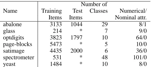
In the test procedure of the vector output SVM we used multiclass classification problems from the UCI Repository of machine learning datasets [3]. The data sets chosen mostly cor-respond to those used by Rifkin et al. [9] to give a well-defined benchmark for comparison. Table 2 shows these sets and their descriptors.
Number of
Name Training Test Classes Numerical/
Items Items Nominal attr.
abalone 3133 1044 29 8/1
glass 214 * 7 9/0
optdigits 3823 1797 10 64/0
page-blocks 5473 * 5 10/0
satimage 4435 2000 6 36/0
spectrometer 531 * 48 101/0
[image:6.612.182.432.70.181.2]yeast 1484 * 10 8/0
Table 2: Parameters of the data sets used in the experiment. * denotes the datasets with no dedicated training and test subsets.
Number of subSVMs
Name all vrs. all one vrs. all vector output
abalone 406 29 1
glass 15 6 1
optdigits 45 10 1
page-blocks 10 5 1
satimage 15 6 1
spectrometer 1128 48 1
[image:6.612.188.424.230.331.2]yeast 45 10 1
Table 3: Number of binary classifiers computed in one multiclass classification problem
Table 3 shows the number of optimisation that need to be solved for the different problems. This is only an indication of the computational effort since they will not all be of the same size. Here we should mention that the elementary binary classifiers in the “one versus one” are generally much simpler than they are in the other methods but their number can be enormous.
In Table 4 the values for the methods “one versus all” and “one versus one” are borrowed from [9] as well. we should emphasize that if the computational complexity of a learner is small then a systematic scanning of the parameter space for an optimal configuration remains sufficiently cheap, so that using a validation set better (and sometimes much better) accuracies can be achieved. For example, the presented test results for the Glass and the Spectrometer use this approach.
6
Conclusions
In this paper we have shown that multiclass learning is expressible in a simple optimization framework and this sort of simplicity not only preserves the accuracy but may improve it. Furthermore it suggests a vector version of the perceptron algorithm with margin (or τ-perceptron) for which the number of updates can be bounded in terms of the optimal margin obtainable [5].
In further research we plan to make a similar reduction of the complexity for structural learning. The simplicity and transparency of the learning methods in this formulation can give strong support to the generalization theory as well by removing unnecessary technical complications.
dimen-Table 4: Test error rates (%). If the data set has dedicated training and test subsets, marked with *, then the table shows the accuracy computed on the given test subset otherwise the presented accuracies are averages computed via 10-fold cross-validation.
Test error rate (%)
vector output Name all vrs. all one vrs. all Perceptron voSVM
abalone * 72.3 79.7 78.6 75.4
glass 30.4 30.8 44.6 24.3
optdigits * 3.8 2.7 10.0 1.5
page-blocks 3.4 3.4 5.5 3.2
satimage * 8.2 7.8 17.3 8.5
spectrometer 42.8 53.7 61.3 35.8
yeast 41.0 40.3 46.8 40.3
sional Hilbert spaces, that is to learn when the input and the output are real valued functions exploiting the simplicity and finiteness of the dual problem.
References
[1] M. Barker and W. Rayens. Partial least squares for discrimination. Journal of
Chemo-metrics, 17:166–173, 2003.
[2] D.P. Bertsekas. Nonlinear Programming. Athena Scienctific, second edition edition, 1999.
[3] C.L. Blake and C.J. Merz. UCI repository of machine learning databases. Uni-versity of California, Irvine, Dept. of Information and Computer Sciences, 1998. http://www.ics.uci.edu/∼mlearn/MLRepository.html.
[4] T. Evgeniou, C.A. Micchelli, and M. Pontil. Learning multiple tasks with kernel methods. Journal of Machine Learning Research, 6(Apr), pages 615–637, 2005. [5] T. Graepel, R. Herbrich, and J. Shawe-Taylor. Generalisation error bounds for sparse
linear classifiers. In Proceedings of the Thirteenth Annual Conference on
Computa-tional Learning Theory, pages 298–303. Morgan Kaufmann Publishers Inc., 2000.
[6] K.C. Kiwiel. Convergence of approximate and incremental subgradient methods for convex optimization. Journal of Optimization, 14, 3:807–840, 2004.
[7] C.A. Micchelli and M. Pontil. Kernels for multi-task learning. In Proc. of the 18-th
Conf. on Neural Information Processing Systems (NIPS’04). 2004.
[8] C.A. Micchelli and M. Pontil. On learning vector-valued functions. Neural
Compu-tation, 17:177–204, 2005.
[9] R. Rifkin and A. Klautau. In defense of one-vs-all classification. Journal of Machine
Learning Research, 5:101–141, 2004.
[10] R. Rosipal, L. J. Trejo, and B. Matthews. Kernel pls-svc for linear and nonlinear classification. In Proceedings of the Twentieth International Conference on Machine
Learning (ICML-2003) Washington DC. 2003.
[11] R. Rosipal and L.J. Trejo. Kernel partial least squares regression in reproducing kernel hilbert space, 2001.