Estimating the spectral response function of the CASI 2

Estimating the spectral response function of the

CASI-2

K. -Y. CHOI and E. J. MILTON

School of Geography, University of Southampton, UK, SO17 1BJ

Abstract

The spectral response function (SRF) of an instrument describes its relative sensitivity to energy of different wavelengths and is normally determined in the laboratory using a tunable laser or a scanning monochromator. In the case of an imaging spectrometer, this procedure is exceptionally difficult and time -consuming as it is necessary to determine the SRF for each of the many hundreds of detectors which make up the sensing array. This paper describes a simplified method to approximate the SRF of the CASI-2 (Compact Airborne Spectrograph Imager), using the same low pressure gas lamps that are used to determine the wavelength calibration of the instrument. The method has been applied to the NERC (Natural Environment Research Council, UK) CASI and results suggest that the SRF is variable across the range of wavelengths sensed, from a full-width half maximum (FWHM) of 2.7 nm at approximately 668 nm, to a FWHM of over 5 nm in the near IR. The results have implications for sensor simulation studies and for applications such as red edge detection.

1

Introduction

Spectral sensitivity is an important parameter of any sensor, and is normally expressed as the spectral response function (SRF) which is the relative responsivity of the sensor to monochromatic radiation of different wavelengths. The SRFs of various broadband sensors are published and these are important to consider when comparing data from different sensors (Teillet et al., 1997; Steven et al., 2003), or when applying physical models such as those used in radiative transfer atmospheric correction (Vermote et al., 1997).

Two main organisations operate Itres CASI-2 systems in the UK: the Natural Environment Research Council (NERC) and the Environment Agency (EA). In neither case is the SRF known, as this is not part of the standard calibration procedure, nor is it supplied by the sensor manufacturer. It has been estimated that direct measurement of the CASI SRF to a resolution of 0.1 nm would take several weeks as it would involve 5,500 separate measurements using five different lasers (pers. comm. Dr Nigel Fox, UK National Physical Laboratory). Clearly, this is not a procedure to be undertaken lightly, nor one which could be repeated very often, yet it is known from routine measurements of the CASI system that slight changes in the optical system of the CASI do occur in normal flight, resulting in changes to the wavelength calibration of up to 0.5 nm (Riedmann, 2003). The impact of these changes on the SRF is unknown.

This paper will describe a method to approximate the SRF of the CASI-2, using an iterative numerical model. The objective of the technique is to estimate the SRF at a number of key wavelengths with acceptable accuracy using the minimum number of laboratory measurements. The new method uses spectral emission peaks from the same low pressure gas lamps that are used for the CASI-2 wavelength calibration. Results will be compared with a generic CASI SRF supplied by the manufacturer as this represents the only other source of information on this important parameter.

2

Data acquisition

2.1

Spectral data collection using the CASI-2

The routine wavelength calibration of the CASI-2 uses four low-pressure gas lamps: Helium, Hydrogen, Mercury, and Oxygen (Riedmann, 2003). Each lamp , depending upon the type of gas, has several spectral emission lines of known centre wavelength. The CASI-2 Sensor Head Unit was mounted with the entrance slit horizontal and an opal glass diffuser attached in front of the objective lens (f/5.6) in order to disperse the narrow beam from the gas lamps and to uniformly illuminate the whole range of the CCD array. The power of the low-pressure gas lamps was very weak, so the CASI integration time was set at 10 s for each frame with a fixed aperture setting. At least 16 measurements were made from each gas lamp, each of which was the sum of four 12-bit frames in the instrument’s on-chip memory. Sixteen summed frames were summed for each gas lamp, the resulting summation of 64 frames in total reduced noise that might have occurred during a series of recordings.

Figure 1 shows an example of the CASI output after the summation. The bright horizontal lines represent spectral peaks across the detector’s spatial pixels. The maximum values of the spectral emission peaks appear around 20,000 DN, whereas most pixels are close to zero after dark signal subtraction. The subtraction of dark current signal from the dataset was important in discriminating the signal from the gas lamps from the instrument-dependent white noise (see the plot on the right of Figure 1).

2.2

Spectral bandwidths of the emission lines

emission lines was measured using an optical spectrum analyser (OSA). The OSA (AQ-6315B), provided by the Opto-Electronics Research Centre (ORC), University of Southampto n, UK, was capable of measuring a wavelength range between 350 and 1750 nm with a spectral resolution of up to 0.01 nm at 1550 nm, depending upon the wavelength span. In order to minimise scattered light from adjacent objects, a fibre optic cable was used to direct the light from the gas lamps into the OSA.

0 1E+0 05 2E+005 3E+ 005

DN values

0

3

6

7

2

1

0

8

1

4

4

1

8

0

2

1

6

2

5

2

2

8

8

Figure 1. CASI-2 image of output from the Helium lamp (612×288 pixels). Top-left pixel position is (0,0). The transect plot on the right is sampled in CCD row of 335

(y-axis represents row numbers of CCD array).

The gas lamps were operated after the same warm-up periods as used for the CASI-2 calibration. Unfortunately, only two out of the four lamps were available for use with the optical fibre. The Oxygen lamp had too low a signal output and the Hydrogen lamp was out of order at the time of the measurements. All the emission lines available for the CASI-2 were measured individually in order to increase the spectral resolution to 0.1 nm with a range of ±20 nm around the centre of peak emission. Figure 2 shows the emission peaks measured by the OSA. All the spectral response curves were symmetrical and their FWHM varied depending on the energy levels and types of gas in the lamp, while the emission peaks were centred exactly on the wavelengths specified by the manufacturer. Signals around each peak were very small, although some noisy signals were observed in low emission peak regions (e.g. plots a and d in Figure 2).

Figure 2. (next page)

Spectral peaks for the dataset used in this study. Centre wavelength of 501.6nm (a), 667.8 nm (b), 701.6 nm (c), and 728.1 nm (d) for Helium tube, and 435.8 nm (e) and

488 496 504 512 520

Wavelength (nm)

0 4E-008 8E-008 1.2E-007 1.6E-007 2E-007 In te n s it y ( n W )

648 656 664 672 680 688

Wavelength (nm)

0 4E-007 8E-007 1.2E-006 1.6E-006 In te n s it y ( n W )

(a) (b)

688 696 704 712 720

Wavelength (nm)

0 1E-006 2E-006 3E-006 4E-006 In te n s it y ( n W )

712 720 728 736 744

Wavelength (nm)

0 1E-007 2E-007 3E-007 In te n s it y ( n W )

(c) (d)

416 424 432 440 448 456

Wavelength (nm)

0 1E-006 2E-006 3E-006 4E-006 5E-006 In te n s it y ( n W )

528 536 544 552 560

Wavelength (nm)

0 1E-006 2E-006 3E-006 In te n s it y ( n W )

3

Methods

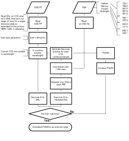
The method developed to approximate the SRF of the CASI-2 involved an iterative process in which each emission curve measured by the OSA was reproduced by successively larger groups of CASI-2 detector elements. After each additional element was added, the predicted emission curve was compared with that measured, and this process continued until the difference between the two was less than a pre-set threshold (Figure 3).

Estimating the CASI SRF in this way involved several assumptions:

• that both the high spectral resolution emission peaks from the gas lamps and the SRF of each detector element in the CASI-2 could be approximated by Gaussian functions.

• that each detector in the CASI-2 array had a wavelength range of spectral response greater than the spectral resolution of the reference data.

• that the wavelength value of each detector element was accurate. In practice, the routine wavelength calibration procedure applied to the CASI-2 involves some wavelength uncertainty (< ~0.3 nm) due to residual error in the polynomial fit of the spectral features and additional uncertainty due to wavelength standard accuracy (< ±0.5 nm).

The first of these assumptions is reasonable, as there are general rules that approximately specify the shape of the SRF: rectangular if a grating is plane, Gaussian if a grating is curved, trapezoidal if a pixel response is rectangular with a curved grating, and triangular if the entrance slit and the detector width are the same size (Hopkinson et al., 2000). In reality, the edge of the function is often rounded due to the effect of diffraction, scattered radiation in the optical system, and non-rectangular detector response. Thus, a Gaussian function is widely accepted for many array detector instruments and is reasonably constant across the detector array within the same optical system (pers. comm. Dr Nigel Fox, NPL).

The Gaussian function, f(λi,σ), can be represented by the centre wavelength and the bandwidth (σ) as a function of the FWHM (Equation 2). The peak of the Gaussian function is assumed to be the centre wavelength of the spectral dimension of the CASI’s CCD. All emission lines measured by the OSA were matched relatively well by Gaussian functions, and expressed by two variables, i.e. the spectral position of the true emission line (a centre wavelength), and a FWHM corresponding to the width of the emission spectrum.

2 2 l n 2 FWHM σ =

⋅ ⋅ Equation 1

2 2

( )

2 ( , ) exp

i

i f

λ λ σ λ σ

− −

⋅

= Equation 2

λI Wavelength [nm]

<λ> Centre wavelength [nm]

σ Bandwidth, or sta ndard deviation

A range of wavelengths was specified surrounding each emission line, normally ±20 nm provided there were no other spectral peaks nearby (except one spectral peak of Helium at 501.6 nm, Figure 2a). Within the wavelength region, the pixel values in the detectors, which were predetermined by the routine wavelength calibration, were normalised, as were the reference spectral peaks from the OSA. As pointed out in the previous section, it was important to eliminate dark current signal from the measured spectra in order to recognise true spectral responses of the emission peaks. Hence, the relative spectral responses of the emission peaks from both measurements were obtained and compared.

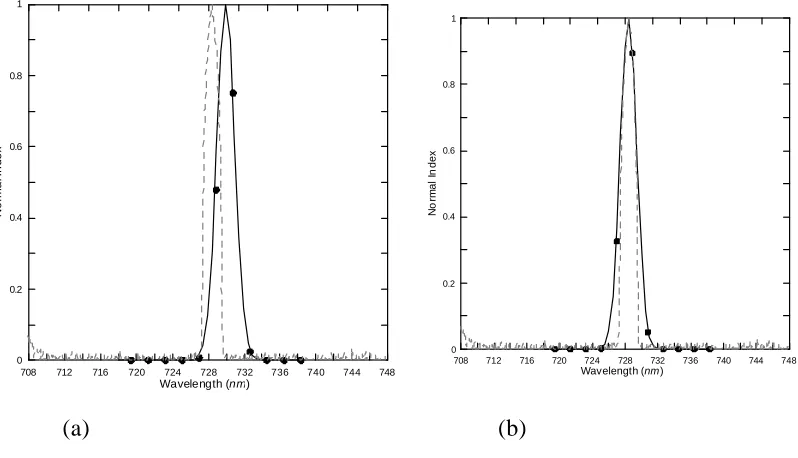
Figure 4 is an example plot of these. From the Gaussian functions fitted to the normalised pixel values of the data from the CASI-2, the emission curve had a wider FWHM than the reference spectrum. This was found for all emission lines available and suggests that the FWHMs of CASI-2 detector elements are wider than those of the reference spectra. If the FWHM of the CASI-2 CCD array had been similar to the sampling resolution of the OSA, i.e. 0.1 nm, the spectral signals from the CASI-2 should have been the same as those of the reference data. A slight wavelength offset in the emission peak in the plot indicated that, as expected, the wavelength determination from the CASI-2 calibration is slightly erroneous, despite still being acceptable according to the manufacturer’s specification.

This disagreement between spectral widths in the two plots, shown in Figure 4a, is a key input parameter of the model. If a CASI-2 detector element had a true FWHM value greater than 0.1 nm at the spectral emission peak, the Gaussian fit of the spectral data points of the CASI-2 supposedly would have been wider than the spectral curve of the reference emission spectrum. The entire reference spectral values within the region would have been scaled with the Gaussian curve and they would have contributed to the total signal received by the CASI-2 detector, i.e. calculation of the area where the data value was greater than zero. To simplify the processing, the FWHM of all the CASI-2 detector elements within the wavelength span around an emission peak was assumed to be uniform. The initial FWHM started at 0.1 nm and increased every 0.01 nm. With a given FWHM, all the CASI-2 detector elements in the spectral region are integrated, and a Gaussian fit applied to the data points. The resulting data points were normalised in order to compare the FWHM with that observed from the CASI-2 spectral responses. The model ran until these FWHM values matched within 0.005 nm.

4

Results

FWHM of Gaussian fit over the estimated data points.

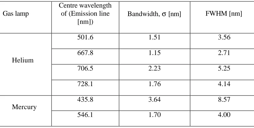
Table 1 lists the model results from the available spectral emission lines. The specification of CASI-2 system states that its minimum spectral resolution, i.e. FWHM, is around 2.2 nm at 650 nm (Itres Research Ltd., 2001). The model result was similar, 2.71 nm at 667.8 nm, and, importantly, it suggests that the FWHM is variable over the wavelength range.

Gas lamp

Centre wavelength of (Emission line

[nm])

Bandwidth, σ [nm] FWHM [nm]

501.6 1.51 3.56

667.8 1.15 2.71

706.5 2.23 5.25

Helium

728.1 1.76 4.14

435.8 3.64 8.57

Mercury

546.1 1.70 4.00

Table 1. The results for CASI-2 FWHM values derived by the method. The value for 435.8 nm is thought to be erroneous for reasons described in the text.

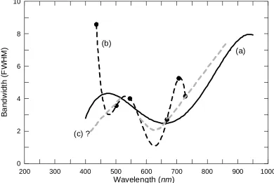
Comparison of the model results with the SRF of the NERC CASI-2 measured conventionally is not possible as this has not been done. However, a typical CASI-2 SRF was measured by Itres Research Ltd (pers. comm. Tyme Wittebrood, Itres Rearch Ltd, 2002) and represented as a fifth order polynomial fit, as a function of wavelength (Figure 5). Unfortunately, the method used for estimating the PSF coefficients by the manufacturer is not known and it does not necessarily represent all CASI-2 models. Nevertheless, such information gives an indication of the CASI-2 SRF and its variability with wavelength.

708 712 716 720 724 728 732 736 740 744 748

Wavelength (nm)

0 0.2 0.4 0.6 0.8 1

N

o

rm

a

l I

n

d

e

x

708 712 716 720 724 728 732 736 740 744 748

Wavelength (nm)

0 0.2 0.4 0.6 0.8 1

N

o

rm

a

l

In

d

e

x

(a) (b)

Figure 4. Comparison between normalised CASI DN values (a) and model output (b). Dashed lines represent one of the emission peaks from Helium (centre wavelength of

728.1nm) as a reference. The FWHM of the Gaussian fit is approximately 4.14 nm. Solid lines are Gaussian fit curves over data values (dots).

5

Conclusions

The SRF technique was much simpler and quicker than conventional laboratory measurements. The numerical model resulted in an credible SRF that compared favourably with that provided by the manufacturer as typical of the CASI-2 design. This suggests that the SRF of the CASI and other array-based sensors could be approximated by this method, thus providing a simple way to check for any changes to the SRF in the interval between laboratory calibrations.

200 300 400 500 600 700 800 900 1000

Wavelength (nm)

0 2 4 6 8 10

B

a

n

d

w

id

th

(

F

W

H

M

) (b) _(a)

(c) ?

Figure 5. Estimated CASI-2 spectral bandwidths. The data for the solid line (a) were provided by S. Achal at Itres Research Ltd. The model output for the NERC CASI is shown in (b) with a best-fit polynomial superimposed. The estimated values below

450 nm are thought to be erroneous for reasons described in the text.

6

Acknowledgements

The authors would like to thank the Natural Environment Research Council (NERC) Airborne Remote Sensing Facility (ARSF) for making the CASI-2 available. The measurements were performed in the calibration laboratory of the School of Geography, University of Southampton, UK. We are also grateful to Junyeong Jang of the Opto-Electronics Research Centre, University of Southampton, UK, for help with the OSA measurements. Development of the method was greatly helped by discussions with Dr Nigel Fox, UK National Physical Laboratory, and Tyme Wittebrood, Itres Research Ltd, Canada.

References

BABEY, S.K. and SOFFER, R.J., 1992. Radiometric calibration of the Compact Airborne Spectrographic Imager (CASI), Canadian Journal of Remote Sensing, 18, 233-242.

COCKS, T., JENSSEN, R., STEWART, A., WILSON, I., SHIELDS, T., 1998. The HyMap airborne hyperspectral sensor: The system, calibration and performance, Proceedings on First EARSEL Workshop on Imaging Spectroscopy, Zurich, 1-6. GREEN, R.O., PAVRI, B.E. and CHRIEN, T.G., 2003, On-orbit radiometric and

spectral calibration characteristics of EO-1 Hyperion derived with an underflight of AVIRIS and in site measurements at Salr de Arizaro, Argentina, IEEE Transactions on Geoscience and Remote Sensing, 41, 1194-1203.

RIEDMANN, M., 2003. Laboratory Calibration of the Compact Airborne Spectrographic Imager (CASI-2).

http://www.soton.ac.uk/~epfs/resources/pdf_pubs/MRCasiCal.pdf

STEVEN, M.D., MALTHUS, T.J., BARET, F., XU, H., CHOPPING, M.J., 2003. Intercalibration of vegetation indices from different sensor systems, Remote Sensing of Environment, 88, 4, 412-422.

TEILLET, P.M., STAENZ, K., WILLIAMS, D.J., 1997. Effects of spectral, spatial, and radiometrix characteristics on remote sensing vegetation indices of forested regions, Remote Sensing of Environment, 61, 1, 139-149.