On the orthogonal distance to class subspaces for high-dimensional data classification

City, University of London Institutional Repository

Citation

:

distance to class subspaces for high-dimensional data classification. Information Sciences, 417, pp. 262-273. doi: 10.1016/j.ins.2017.07.019

This is the accepted version of the paper.

This version of the publication may differ from the final published

version.

Permanent repository link:

Link to published version

:

Copyright and reuse:

City Research Online aims to make research

outputs of City, University of London available to a wider audience.

Copyright and Moral Rights remain with the author(s) and/or copyright

holders. URLs from City Research Online may be freely distributed and

linked to.

City Research Online: http://openaccess.city.ac.uk/ [email protected]

On the orthogonal distance to class subspaces for

high-dimensional data classification

Rui Zhua, Jing-Hao Xuea,∗

a_{Department of Statistical Science, University College London, London WC1E 6BT, UK}

Abstract

The orthogonal distance from an instance to the subspace of a class is a

key metric for pattern classification by the class subspace-based methods.

There is a close relationship between the orthogonal distance and the residual

standard deviation of a test instance from the class subspace. In this paper,

we shall show that an established and widely-used relationship, between the

residual standard deviation and the sum of squares of the residual PC scores,

is not precise, and thus can lead to incorrect results, for the inference of

high-dimensional data which nowadays are common in practice.

Keywords: Classification, high-dimensional data, orthogonal distance,

principal component analysis (PCA), soft independent modelling of class

analogy (SIMCA).

1. Introduction

1

In class subspace-based classification methods, a subspace is first learned

2

in the training phase for each class separately from its training data. Then in

3

∗_{Corresponding author. Tel.: +44-20-7679-1863; Fax: +44-20-3108-3105} Email addresses: [email protected](Rui Zhu),[email protected]

the test phase, these learned class subspaces are utilised to predict the label

4

of a new test instance, by comparing the distances from the test instance to

5

the class subspaces, in terms of certain distance metrics. For example, in a

6

widely-used classifier for spectral data called soft independent modelling of

7

class analogy (SIMCA) [28], principal component (PC) subspaces are learned

8

for individual classes. Similar to SIMCA, another popular PCA-based

clas-9

sification approach has been extensively adopted in process control in

engi-10

neering, such as fault detection and diagnosis [20, 16, 15, 25]. Besides

classi-11

fication methods, some clustering methods also aim to seek low-dimensional

12

subspaces for better clustering results [13, 23, 22].

13

In the above two classification approaches, associated with the PC

sub-14

spaces, two distance metrics (or statistics) are often adopted to achieve

pat-15

tern classification [3, 17, 18, 20, 16, 15, 25, 29]: 1) the orthogonal distance

16

(OD), also known as the Q-statistic or the squared prediction error, i.e. the

17

squared orthogonal Euclidean distance from a test instance to a PC subspace;

18

and 2) the score distance (SD), also known as the Hotelling’s T2 statistic,

19

i.e. the squared Mahalanobis distance from the projection of a test instance

20

to the centre of a PC subspace [17]. The distributions of OD and SD have

21

also been studied extensively, in order to find a proper acceptance area for

22

classification; recent work includes [17], [18], [19], [30] and [21]. Also in

23

recent years, a linear combination of these two distances is often used to

24

classify a test instance: the test instance is assigned to the class with the

25

minimum value of the linear combination [3].

26

There is a close relationship between the OD (from a test instance to a

27

class subspace) and the residual standard deviation of the test instance to

the class subspace. Moreover, Maesschalck et al. [9] show that the residual

29

standard deviation based on the residual matrix can be equivalently

calcu-30

lated from using the residual PC scores based on the PC score matrix. This

31

work has been cited over a hundred times, including methodological

develop-32

ments [4, 10, 8], reviews [24, 14] and applications [5, 2, 6, 27, 7]. The recent

33

work studying the distributions of OD and SD [17, 18, 19] also adopted the

34

formulae in [9] following [10].

35

However in this paper, we shall point out that the relationship presented

36

in [9], between the residual standard deviation and the sum of squares of the

37

residual PC scores, is notprecise for the inference of high-dimensional data.

38

To distinguish the training and test scenarios, we shall establish the

no-39

tation of two ODs, respectively, as follows.

40

1. The OD vk,l _{from the training instance l to the subspace of class k}

41

that was learned from all training instances. It is closely related to

42

the residual standard deviation sk,0 _{of class k, which will be defined in}

43

Section 2.1.

44

2. The OD vk,new from the new test instance to the subspace of class k.

45

It is closely related to the residual standard deviationsk,new _{of the new}

46

test instance to class k, which will be defined in Section 2.2.

47

In short, the difference between vk,l _{and v}k,new _{is that v}k,l _{is the OD for the}

48

training instance while vk,new _{is the OD for the test instance.}

49

The contributions of this paper are as follows. First, although

Maess-50

chalck et al. [9] establish formulae for sk,0 _{and s}k,new _{using the residual PC}

51

scores, we shall show that their formula for sk,new _{is only precise when the}

52

training data of classkhave more instances than predictor features, i.e. when

the number of instances (denoted bynk) is larger than the number of features

54

(denoted by p). In other words, we shall show that, when the training data

55

of class k are high-dimensional (i.e. nk ≤ p, also called “large p, small n” in

56

the statistical literature), the calculation of sk,new in [9] is not precise.

57

Second, because of the above results, we shall point out that, for

high-58

dimensional data, although the OD vk,l can be accurately calculated by

fol-59

lowing the (precise) formula of the residual standard deviation sk,0 _{in [9],}

60

the OD vk,new cannot be accurately calculated by following the (imprecise)

61

formulae of the residual standard deviation sk,new _{in [9]. Consequently,}

in-62

ference results of the studies that calculated the ODs for high-dimensional

63

data using the formulae in [9] can be imprecise.

64

Because nowadays high-dimensional data are commonly present in

pattern-65

recognition tasks, it is of great interest to practitioners to point out the

im-66

precise calculation of the ODs for high-dimensional data if we follow the

67

formulae in [9], as well as to suggest that the formulae in [28] should be

68

adopted in this “large p, small n” paradigm.

69

2. The calculations of OD in [9]

70

The following calculations are all for class k. The subscripts p, q and r

71

denote the number of columns in matrices U,D,V andT; for example,Vp

72

indicates that there are pcolumns in matrix Vp of class k.

73

2.1. The training phase of class k

74

Suppose X ∈ _Rnk×p _{is the training set of class k, in which there are n}

k

75

training instances (or say training samples) and each instance is represented

apply the reduced singular value decomposition (SVD) to the column-centred

78

training set X(c):

79

X(c)=UqDq(Vq)T , (1)

where Uq ∈Rnk×q and Vq ∈ Rp×q are the two matrices containing left and

80

right singular vectors as columns, respectively, and Dq ∈Rq×q is a diagonal

81

matrix with singular values {λ1 ≥ λ2 ≥ · · · ≥ λq ≥ 0}. The parameter

82

q ≤min(p, nk−1) is the rank of X(c).

83

In PCA, the rows of Tq = UqDq ∈ Rnk×q are known as PC scores and

84

the columns of Vq are known as PCs. Suppose the first r (r ≤ q) PCs are

85

selected to build the PC subspace for class k, then

86

X(c) =Tr(Vr)T +E , (2)

whereTr ∈Rnk×r;Vr∈Rp×r; andE∈Rnk×pis the training residual matrix

87

of class k.

88

In [9], the residual standard deviation of classkis expressed in two forms:

89

sk,0 =

v u u t

1 DoFk,0

nk

X

l=1

p X

j=1

(elj)2 = v u u t

1 DoFk,0

nk

X

l=1

q X

i=r+1

(tli)2 (3)

where DoFk,0 = (q−r)(nk−r−1), elj is the (l, j)-entry of residual matrix

90

E representing the residual of thelth instance for thejth variable, and tli is

91

the (l, i)-entry of score matrix Tq representing the score of the lth instance

92

for the ith PC.

93

The OD from thelth training instance to the subspace of class k,vk,l_{, is}

originally defined as Pp

j=1(elj)

2_{. Thus} Pnk

l=1v

k,l _{is proportional to (s}k,0₎2_,

95

nk

X

l=1

vk,l = (sk,0)2(q−r)(nk−r−1). (4)

In [9], it follows from (3) that Pnk

l=1v

k,l _{can be calculated as}

96

nk

X

l=1

vk,l =

nk

X

l=1

q X

i=r+1

(tli)2 . (5)

2.2. The test phase for class k

97

In the test (prediction) phase, to decide whether a new instance xnew

98

belongs to class k or not, xnew _{is first centred by using the means of the}

99

variables of the training dataX of classk, and the result is denoted byxk,new_(c) .

100

Then projectingxk,new_(c) to the PC subspace of classk with the selectedrPCs,

101

we can obtain

102

xk,new_(c) =tk,new_r (Vr)T +ek,new , (6)

where tk,new

r ∈ R1

×r _{and e}k,new _∈

R1×p are two vectors of the PC score and 103

the residual, respectively, of the new instance when it is fitted to the subspace

104

of class k.

105

In [9], the residual standard deviation of the new instance is also expressed

106

in two forms:

107

sk,new =

v u u t

1

DoFk,new

p X

j=1

(ek,new_j )2 ₌

v u u t

1

DoFk,new

q X

i=r+1

(tk,new_i )2_{, (7)}

where DoFk,new = (q−r), ek,new_j and tk,new_i denote the jth element of the

residual vector ek,new _{and the ith element of the PC score vector t}k,new

r ,

109

respectively.

110

The OD from the new instance to the subspace of class k, vk,new_{, is}

111

originally defined as Pp

j=1(e

k,new

j )2. Thus vk,new is proportional to (sk,new)2,

112

vk,new = (sk,new)2(q−r). (8)

In [9], it follows from (7) that vk,new _{can be written as}

113

vk,new =

q X

i=r+1

(tk,new_i )2 . (9)

To determine the class of xnew_{, the residual standard deviation s}k,new

114

of xnew _{is compared to the residual standard deviation s}k,0 _{of the training}

115

instances of classk [9]. The F-test statistic used in [9] to determine whether

116

the two residual variances are significantly different is expressed as

117

Fk,new = (s

k,new₎2

(sk,0₎2 = Pq

i=r+1(t

k,new

i )2 (nk−r−1)

Pnk

l=1

Pq

i=r+1(tli)2

. (10)

3. Discussion of vk,l _{and v}k,new 118

The calculations forvk,0 _andvk,new _{in [9] use formulae (5) and (9),}

respec-119

tively. We shall show that, while formula (5) is correct for both the cases of

120

nk> p and nk ≤p, formula (9) is only valid when nk > p.

121

3.1. vk,l

122

The OD vk,l _{is originally defined on the basis of the residual matrix E.}

123

The calculation of vk,l _{in (5), which was defined in [9], is on the basis of the}

PC score matrix Tr. This is due to the relationship that

125

nk

X

l=1

p X

j=1

(elj)2 =

nk

X

l=1

q X

i=r+1

(tli)2 . (11)

This relationship is true for both the cases of nk> p and nk ≤p, as we shall

126

show in the following two subsections, respectively.

127

3.1.1. nk> p

128

When nk > p, we have q = p (assume that no feature is a linear

com-129

bination of others), and thus Vq ∈Rp×p is a square matrix. It follows that

130

Vq(Vq)T = (Vq)TVq=Ip.

131

Let xl

(c) ∈R

1×p _{denote the l-th training instance in class k, i.e. the l-th}

row of X(c). For every xl(c) (l = 1, . . . , nk), we have xl(c) =x l

(c)Vq(Vq)T and

p X

j=1

(elj)2 =||xl(c)−x l

(c)Vr(Vr)T||22

=||xl_(c)Vq(Vq)T −xl(c)Vr(Vr)T||22

=||tl_q(Vq)T −tlr(Vr)T||22

=

q X

i=r+1

(tli)2 , (12)

where || · ||2 denotes the Euclidean norm of a vector, and tlq and tlr are the

132

lth row of Tq and Tr, respectively. Therefore (11) and thus (5) are correct

133

when nk> p.

3.1.2. nk≤p

135

Whennk≤p, we haveq= rank(X(c))≤nk−1< p, and thus Vq ∈Rp×q

136

is not square. It follows that (Vq)TVq =Iq but Vq(Vq)T 6=Ip.

137

Suppose we apply the full SVD toX(c):

138

X(c) =UnkDˆp(Vp)

T

, (13)

where Unk ∈ R

nk×nk _{and V}

p ∈ Rp×p denote the two matrices containing nk

139

left and p right singular vectors as columns, respectively, and ˆDp ∈ Rnk×p 140

is a matrix with singular values {λ1 ≥ λ2 ≥ · · · ≥ λnk−1 ≥ λnk = 0} on the

141

main diagonal.

142

To make the explanation more clear, we expand ˆDp ∈Rnk×p to a square

143

matrix Dp ∈ Rp×p by adding zeros because the singular values associated 144

with the last (p−q) PCs are zeros when nk ≤ p. Matrix Unk ∈ R

nk×nk _is

145

also expanded to Up ∈Rnk×p using (p−nk) unit-length column vectors that

146

are randomly calculated to be orthogonal to the previous column vectors.

147

Thus we have

148

X(c)=UnkDˆp(Vp)

T _=U

pDp(Vp)T, (14)

where Up ∈Rnk×p and Vp ∈Rp×p denote the matrices containing pleft and

149

p right singular vectors, respectively, and Dp ∈ Rp×p is a diagonal matrix 150

with singular values {λ1 ≥ λ2 ≥ · · · ≥ λq ≥ λq+1 = · · · = λp = 0}. Since

151

Vp ∈Rp×p is square, we have Vp(Vp)T = (Vp)TVp =Ip.

152

LetTp = UpDp ∈ Rnk×p denote the PC scores. Let tli denote the (l, i

)-153

entry of score matrixTp representing the score of thelth instance for theith

154

PC.

Letml _{denote the residual from using the firstqPCs to reconstructx}l (c):

ml =xl_(c)−x₍l_c)Vq(Vq)T. We calculate the sum of squares of the residuals

in ml _{for the l-th instance:}

||ml||2₂ =||xl_(c)−xl_(c)Vq(Vq)T||22

=||xl_(c)Vp(Vp)T −xl(c)Vq(Vq)T||22

=||tl_p(Vp)T −tlq(Vq)T||22 . (15)

The sum of ||ml_||2

2 for all nk training instances is

156

nk

X

l=1

||ml||2

2 =

nk

X

l=1

p X

i=q+1

(tli)2 = p X

i=q+1

(λi)2 . (16)

The second equation in (16) can be shown as follows. X(c)=UpDp(Vp)T ⇒

157

(Up)TX(c)Vp =Dp ⇒(Up)TTp =Dp. For the ith singular valueλi in Dp,

158

we have (λi)2 = (uTi ti)2 =tTi uiuTi ti =tTi ti = Pnk

l=1(tli)2, whereui andti are

159

the ith columns ofUp and Tp, respectively.

160

Since the last (p−q) singular values are zeros, Pnk

l=1||ml||22 = 0. Because

161

each term in the sum Pnk

l=1||m

l_||2

2 is nonnegative, ||ml||22 = 0 for all l (l =

162

1, . . . , nk). Thus we have xl(c) =x(lc)Vq(Vq)T, which means that the first q

163

PCs can perfectly reconstruct the training instances in class k. Using the

164

same proof as in (12), we can show that (11) and thus (5) are also true for

165

nk≤p.

166

Therefore,vk,l _{can be correctly calculated by using (5) for both the cases}

167

of nk> p and nk ≤p.

3.2. vk,new

169

The ODvk,new_{is originally defined in terms of the residual vectore}k,new_[28],

170

while following [9] vk,new is formulated in (9) by using the PC score tk,new_r of

171

the new sample. We shall show that the formula (9) is valid when nk > p

172

but not valid when nk ≤p, in the following two subsections, respectively.

173

3.2.1. nk> p

174

Whennk> p, we haveq =p, and thusVq ∈Rp×p is a square matrix. As

175

before, Vq(Vq)T = (Vq)TVq =Ip. Since xk,new_(c) =xk,new_(c) Vq(Vq)T, we have

176

p X

j=1

(ek,new_j )2 =

q X

i=r+1

(tk,new_i )2 . (17)

Using a proof similar to (12) by replacing xl_(c) with xk,new_(c) , we can readily

177

show that (17) and thus (9) are correct for nk > p.

178

3.2.2. nk≤p

179

When nk ≤ p, we have q = rank(X(c)) < p, and thus Vq ∈ Rp×q is not

180

square. Again, it follows that (Vq)TVq=Iq but Vq(Vq)T 6=Ip.

181

Letmk,new denote the residual from using theqPC vectors to reconstruct

xk,new_(c) : mk,new _=xk,new

(c) −x

k,new

(c) Vq(Vq)

of the residuals in mk,new_:

||mk,new||2₂ =||xk,new_(c) −xk,new_(c) Vq(Vq)T||22

=||xk,new_(c) Vp(Vp)T −xk,new_(c) Vq(Vq)T||22

=||tk,new_p (Vp)T −tk,newq (Vq)T||22

=

p X

i=q+1

(tk,new_i )2 , (18)

where || · ||2 denotes the Euclidean norm of a vector.

182

However, unlike the case for the training data, Pp

i=q+1(t

k,new

i )2 is not

183

necessarily equal to zero for a p-dimensional test instance. Thus xk,new_(c) 6=

184

xk,new_(c) Vq(Vq)T, which means that the new test instance cannot be perfectly

185

reconstructed by the first q PC vectors.

186

Hence, if we rewrite

xk,new_(c) =xk,new_(c) Vq(Vq)T +mk,new

=xk,new_(c) Vr(Vr)T + (xk,new_(c) Vq(Vq)T −xk,new_(c) Vr(Vr)T) +mk,new ,

(19)

we have

ek,new = (xk,new_(c) Vq(Vq)T −xk,new_(c) Vr(Vr)T) +mk,new

= (tk,new_q (Vq)T −tk,newr (Vr)T) + (tk,newp (Vp)T −tk,newq (Vq)T)

and

p X

j=1

(ek,new_j )2 =||ek,new||2₂

=||tk,new_p (Vp)T −tk,newr (Vr)T||22

=

p X

i=r+1

(tk,new_i )2

=

q X

i=r+1

(tk,new_i )2+

p X

i=q+1

(tk,new_i )2 . (21)

Comparing (21) with (17), we can find an additional term Pp

i=q+1(t

k,new

i )2 in

187

(21), and this term may not be zero. It follows that (17) and thus (9) are

188

not valid when nk ≤p.

189

Whennk ≤p,Pp_i=q+1(tk,newi )2 is hard to estimate because the last (p−q)

190

PCs are randomly calculated by satisfying the orthogonal condition.

Never-191

theless, it can be harmful to the classification of the new instance of

high-192

dimensional “large p, small n” data, if we use (9) to calculate vk,new _which

193

omitsPp

i=q+1(t

k,new

i )2, because the decision making for classification is based

194

on vk,new_.

195

4. Experiments

196

In the following experiments, take SIMCA as an example: we compare

197

the SIMCA with the OD defined originally in [28] (denoted by SIMCA) and

198

the SIMCA with the OD calculated by following [9] (denoted by SIMCA-D),

199

evaluating them on both simulated and real datasets. We aim to show that

200

the additional term Pp

i=q+1(t

k,new

i )2 can be important for classifying

dimensional data. To simplify the experiment settings, we discuss the effect

202

of Pp

i=q+1(t

k,new

i )2 on two-class classification in the experiments. The effect

203

of Pp

i=q+1(t

k,new

i )2 on multi-class classification can be readily extended.

204

4.1. Classification rule

205

New test instances can be classified by following the classification rule of

206

the robust SIMCA (RSIMCA) [3], which is a linear combination of the OD

207

and the SD of a new test instance (Here our notations of OD and SD are

208

both for squared distances). That is, a new test instance is classified to the

209

class with the minimum value of

210

γOD

k

ck OD

+ (1−γ)SD

k

ck SD

, (22)

where ODk =vk,new; SDk = (tk,new_r )TΛ−_r1tk,new_r , in which Λr is the diagonal

211

matrix of the r largest eigenvalues for the PC subspace; ck

SD = χ2r;0.975; and

212

ck_OD = (ˆµ+ ˆσz0.975)3, in which ˆµ and ˆσ are the mean and the standard

213

deviation of the square roots of vk,l_.

214

Since ODk is the only term that is different between SIMCA and

SIMCA-215

D, the value of the second term in (22) does not affect the difference between

216

SIMCA and SIMCA-D. We force the value of the second term in (22) to zero

217

by setting γ = 1, to simplify the experiments.

218

4.2. Validation criterion

219

We use the overall misclassification percentage (MP) as the validation

220

criterion following the experiments in [3]. We use the one-assignment-rule

221

suggested in [3], i.e. a test sample is assigned to one of the known classes

with the smallest F-value, to simplify the calculation of the MP and obtain

223

unambiguous final results. The MP is defined as

224

MP =

K X

k=1

nt_k/Nt , (23)

where nt

k denotes the the number of wrongly assigned test samples in class

225

k and Nt denotes the total number of test samples.

226

4.3. Datasets

227

4.3.1. Simulated datasets

228

Simulated datasets are generated by following the experiments in [18].

229

Assume that a sample vectorxis the sum of two independent normal random

230

components:

231

x=δ+, (24)

where

232

δ ∼N(µ,Σ) and∼N(0, σ2I) . (25)

Based on the above assumption, the samples of the two classes are drawn

233

from N(µ₁,Σ1+σ12I) and N(µ2,Σ2+σ22I), respectively.

234

Two sets of parameters, simulation A and simulation B, are devised to

235

show the following two situations, respectively: 1) Pp

i=q+1(t

k,new

i )2 is not

236

important for classification; and 2) Pp

i=q+1(t

k,new

i )2 may be important for

237

classification. The details of the two simulation settings are summarised in

238

Table 1.

239

For each simulation setting, we generate 20 datasets with different nk/p

240

ratios to explore the difference between SIMCA and SIMCA-D with respect

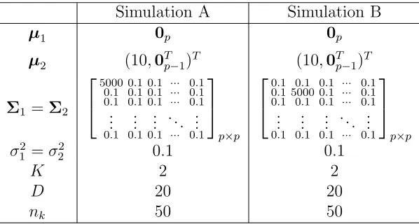
Table 1: Simulation settings. Notation: K, number of classes;D, number of datasets;nk,

number of samples in each class

Simulation A Simulation B

µ₁ 0p 0p

µ₂ (10,0T

p−1)T (10,0Tp−1)T

Σ1 =Σ2 



5000 0.1 0.1 ··· 0.1 0.1 0.1 0.1 ··· 0.1 0.1 0.1 0.1 ··· 0.1

..

. ... ... ... ...

0.1 0.1 0.1 ··· 0.1 



p×p





0.1 0.1 0.1 ··· 0.1 0.1 5000 0.1 ··· 0.1 0.1 0.1 0.1 ··· 0.1

..

. ... ... ... ...

0.1 0.1 0.1 ··· 0.1 



p×p

σ2₁ =σ2₂ 0.1 0.1

K 2 2

D 20 20

nk 50 50

top. In each dataset, 50 samples are generated for each class, from which 25

242

samples are selected as the training set and the rest as the test set, i.e. n1

243

and n2 are fixed to 25 for all the datasets. The 20nk/pratios are 1.5, 1, 0.7,

244

0.5, 0.3, 0.1, 0.09, 0.08, 0.07, 0.06, 0.05, 0.04, 0.03, 0.02, 0.01, 0.009, 0.008,

245

0.007, 0.006 and 0.005; and the corresponding p’s are 17, 25, 36, 50, 83, 250,

246

278, 313, 417, 500, 625, 833, 1250, 2500, 2778, 3125, 3571, 4167 and 5000.

247

Among these settings, nk/p = 1.5 (i.e. p = 17) indicates a low-dimensional

248

dataset while other ratios indicate high-dimensional datasets.

249

It is clear in Table 1 that the only difference between simulation A and

250

simulation B is the values of Σ1 and Σ2, which determines the importance

251

of Pp

i=q+1(t

k,new

i )2 for classification. In both simulations, the first

dimen-252

sions of the feature vectors contain major discriminative information since

253

µ11 = 0 and µ21 = 10, while other dimensions contain little discriminative

254

information since µ1i = µ2i = 0 (i 6= 1). Therefore, the variance of the

255

first dimension determines how the discriminative information between two

classes is distributed to the PCs. The discriminative information left in the

257

residuals for classification is determined by the discriminative information in

258

the first few PCs used in the class subspace.

259

If the first dimension has the largest variance and the discriminative

in-260

formation is concentrated on the first PC which is definitely used in the class

261

subspace, i.e. (Σ1)11 = (Σ2)11 = 5000 in simulation A, then Pp

j=1(e

k,new

j )2

262

is not very discriminative (or say unimportant for classification) and so is

263

Pp

i=q+1(t

k,new

i )2. In contrast, if the first dimension has a small variance and

264

contributes randomly to the PCs, i.e. (Σ1)11= (Σ2)11 = 0.1 in simulation B,

265

then the discriminative information may not be concentrated on the first few

266

PCs that are used in the class subspace. In this case, Pp

j=1(e

k,new

j )2 can be

267

discriminative (or say important for classification) and so bePp

i=q+1(t

k,new

i )2.

268

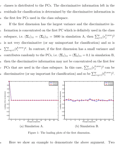
2 4 6 8 10 12 14 16 18 20 22 24

−1 −0.8 −0.6 −0.4 −0.2 0 0.2 0.4 0.6 0.8 1 Principal components

Loadings of the 1st dimension

Group1 Group2

(a) Simulation A.

2 4 6 8 10 12 14 16 18 20 22 24

−1 −0.8 −0.6 −0.4 −0.2 0 0.2 0.4 0.6 0.8 1 Principal components

Loadings of the 1st dimension

Group1 Group2

(b) Simulation B.

Figure 1: The loading plots of the first dimension.

Here we show an example to demonstrate the above argument. Two

269

datasets with p= 1250 are generated. Applying PCA separately to the two

270

classes of each dataset, we obtain the PCs for each class. We record the

first entries of all the PCs in each class, i.e. Vq(1,:), and plot them against

272

the PCs sorted in decreasing order of singular values, as shown in Figure 1

273

for simulation A and simulation B, respectively. These loadings indicate the

274

contributions of the first dimensions of the feature vectors to the PCs.

275

In simulation A, the absolute loadings of the first PC are close to one while

276

those of other PCs are close to zeros, which indicates that the discriminative

277

information between the two classes is concentrated on the the first PC.

278

Since the first PC is definitely used to build the class subspace,Pp

j=1(e

k,new

j )2

279

contains little discriminative information from the first dimension. Thus, as

280

a part of Pp

j=1(e

k,new

j )2,

Pp

i=q+1(t

k,new

i )2 is not important for classification.

281

In simulation B, the loadings are distributed randomly around zero, which

282

indicates that the discriminative information is spread over all PCs.

There-283

fore, Pp

j=1(e

k,new

j )2 may contain discriminative information important for

284

classification and so be Pp

i=q+1(t

k,new

i )2.

285

4.3.2. Real datasets

286

A low-dimensional dataset (the iris data) and three high-dimensional

287

datasets (the Phenyl data, the meat data and the fat data) are used in

288

the experiments.

289

The iris dataset [12] contains 150 samples with three classes: each class

290

contains 50 samples. Each sample is described by four features.

291

The Phenyl dataset is provided in the R package, ‘chemometrics’. The

292

dataset consists of 600 mass spectrum of chemical components, with 300

293

compounds contain the phenyl substructure and 300 compounds do not

con-294

tain the substructure. Each spectra contains 658 mass spectral features. We

with 50 contain the phenyl substructure and 50 do not contain the structure.

297

The meat dataset [1] consists of 108 spectra of meat spectra measured at

298

1051 wavelengths, with 55 chicken samples and 54 turkey samples.

299

The fat dataset [11] consists of 193 spectra of finely chopped meat, with

300

122 meat samples of less than 20% fat and 71 samples of larger than 20%

301

fat. Each spectrum is measured at 100 wavelengths.

302

4.4. Experiment settings

303

For the iris data and the Phenyl data, we randomly select 25 samples

304

from each class to generate the training set. For the meat data, we randomly

305

select 27 chicken samples and 27 turkey samples for training. For the fat

306

data, we randomly select 35 samples of less than 20% fat and 35 samples

307

of larger than 20% fat for training. The remaining samples of each dataset

308

generate the test set.

309

We repeat this procedure 100 times and perform the two methods, SIMCA

310

and SIMCA-D, on each training-test split.

311

In both methods, the number of PCs are chosen using the criterion that

312

the variance explained is more than 85% for all classes. Thus the numbers

313

of PCs, r, are the same for the two methods.

314

4.5. Results

315

4.5.1. Simulated datasets

316

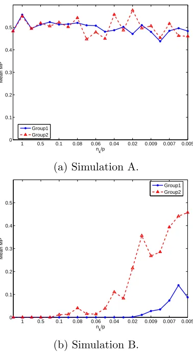
To explore the effect of the nk/p ratio on the performances of SIMCA

317

and SIMCA-D, we plot the the mean MP against the nk/pratio in Figure 2

318

for simulation A and simulation B, respectively. It is clear that the mean

319

MPs of SIMCA and SIMCA-D are the same when nk/p = 1.5, i.e. in the

1 0.5 0.1 0.08 0.06 0.04 0.02 0.009 0.007 0.005 0

0.1 0.2 0.3 0.4 0.5

nk/p

Mean MP

Group1 Group2

(a) Simulation A.

1 0.5 0.1 0.08 0.06 0.04 0.02 0.009 0.007 0.005

0 0.1 0.2 0.3 0.4 0.5

n_k/p

Mean MP

Group1 Group2

(b) Simulation B.

low-dimensional situation, in each of the simulation settings, as indicated by

321

the leftmost points in each panel of Figure 2.

322

However, the relative performances of SIMCA and SIMCA-D are different

323

for the two simulations whennk/p≤1, i.e. in the high-dimensional situation.

324

In simulation A, the mean MPs of the two methods are similar for allnk/p

325

ratios, as shown in Figure 2a. This indicates that ignoring Pp

i=q+1(t

k,new

i )2

326

in the calculation of the OD does not affect the classification results in this

327

simulation, because in this case Pp

i=q+1(t

k,new

i )2 is not important for

classifi-328

cation. In addition, since the residuals are not discriminative, the mean MP

329

varies around 0.5.

330

In simulation B, the difference between the mean MPs of the two methods

331

becomes larger as nk/p becomes smaller (i.e. when the data are higher

di-332

mensional), as shown in Figure 2b. Since in this simulation the first few PCs

333

used in class subspaces contain little discriminative information, the residual

334

Pp

j=1(e

k,new

j )2 is important for classification. SIMCA performs pretty well

335

for almost all the nk/p ratios because Pp

j=1(e

k,new

j )2 captures the

discrimi-336

native information for classification. In contrast, SIMCA-D, which only uses

337

Pq

i=r+1(t

k,new

i )2 for classification and ignores Pp

i=q+1(t

k,new

i )2, cannot capture

338

the discriminative information in Pp

i=q+1(t

k,new

i )2 and can be suboptimal in

339

classification, especially when nk/pis small (i.e. when the data dimension is

340

high). For example, the mean MP of SIMCA-D worsens to around 0.4 when

341

nk/p decreases to 0.008.

342

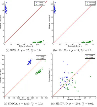
In addition for simulation B, we show an example of howPp

i=q+1(t

k,new

i )2

343

affects the classification performance using the Coomans’ plots. Figure 3

344

shows the Coomans’ plots of the test samples on one training-test split of

0 20 40 60 80 100 120 0

20 40 60 80 100 120

Distance to Group 1

Distance to Group 2

Group 1 Group 2

(a) SIMCA.p= 17, nk

p = 1.5.

0 20 40 60 80 100 120

0 20 40 60 80 100 120

Distance to Group 1

Distance to Group 2

Group 1 Group 2

(b) SIMCA-D.p= 17, nk

p = 1.5.

0 50 100 150 200 250 300 350 400 450 0

50 100 150 200 250 300 350 400 450

Distance to Group 1

Distance to Group 2

Group 1 Group 2

(c) SIMCA. p= 1250, nk

p = 0.02.

0 2 4 6 8 10 12 14 16

0 2 4 6 8 10 12 14 16

Distance to Group 1

Distance to Group 2

Group 1 Group 2

(d) SIMCA-D.p= 1250, nk

p = 0.02.

each simulated dataset. The Coomans’ plot [26] shows the orthogonal

dis-346

tance from the test samples to two class subspaces at the same time. In

347

our experiments, the horizontal and vertical axes denote the ODs to Group

348

1 and Group 2, respectively. In Figure 3, the red reference line divides the

349

Coomans’ plot into two parts: in the upper triangular part, the distance to

350

Group 1 is smaller than that to Group 2; in the lower triangular part, it is

351

the other way around.

352

Since SIMCA and SIMCA-D have the sameq and r, the Coomans’ plots

353

reflect the difference between the ODs of these two methods.

354

When nk/p = 1.5 (i.e. low-dimensional), the Coomans’ plots of the two

355

methods are the same. Whennk/p= 0.02 (i.e. high-dimensional), the Coomans’

356

plots of the two methods are different. We observe large differences between

357

the values of ODs in Figure 3c and Figure 3d, which indicates that the value

358

of Pp

i=q+1(t

k,new

i )2 is large. Including Pp

i=q+1(t

k,new

i )2 can perfectly separate

359

the two groups as shown in Figure 3c; however, omittingPp

i=q+1(t

k,new

i )2

re-360

sults in a mixture of the two groups as shown in Figure 3d. This indicates

361

that the additional termPp

i=q+1(t

k,new

i )2 is important for classification in this

362

high-dimensional simulated dataset.

363

4.5.2. Real datasets

364

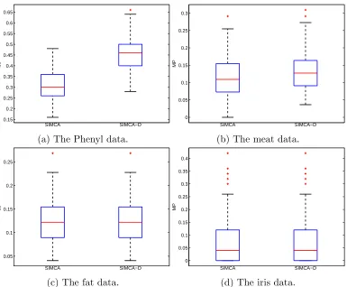
Figure 4 shows the box plots of the MP for the real datasets. In the

high-365

dimensional Phenyl data and the high-dimensional meat data, SIMCA-D

366

provides worse classification performance than the original SIMCA. However,

367

in the high-dimensional fat data, SIMCA-D and SIMCA provides the same

368

classification results. The results suggest that SIMCA-D can provide worse

369

classification results than SIMCA for some high-dimensional real datasets. In

0.15 0.2 0.25 0.3 0.35 0.4 0.45 0.5 0.55 0.6 0.65

SIMCA SIMCA−D

MP

(a) The Phenyl data.

0 0.05 0.1 0.15 0.2 0.25 0.3

SIMCA SIMCA−D

MP

(b) The meat data.

0.05 0.1 0.15 0.2 0.25

SIMCA SIMCA−D

MP

(c) The fat data.

0 0.05 0.1 0.15 0.2 0.25 0.3 0.35 0.4

SIMCA SIMCA−D

MP

(d) The iris data.

the low-dimensional iris dataset, the two methods provide the same results.

371

This pattern for the real datasets is consistent with that for the simulated

372

datasets.

373

5. Conclusion

374

We have investigated the formulae in [9] of calculating two ODs,vk,l and

375

vk,new_{. We have shown that the formula forv}k,new _{in [9] is not valid for}

high-376

dimensional data (i.e. whennk ≤p). The experiments on both the simulated

377

datasets and the real datasets have confirmed that the formula following [9]

378

can result in worse classification performance than the original one in [28].

379

Therefore, we suggest that the original formulae in [28] for calculating the

380

ODs, rather than the formulae in [9], should be used for the classification

381

of high-dimensional data which have more features than samples (i.e. when

382

nk≤p).

383

Acknowledgment

384

The authors would like to thank the reviewers for their constructive

com-385

ments.

386

References

387

[1] T. Arnalds, J. McElhinney, T. Fearn, G. Downey, A hierarchical

dis-388

criminant analysis for species identification in raw meat by visible and

389

near infrared spectroscopy, Journal of Near Infrared Spectroscopy 12 (3)

390

(2004) 183–188.

[2] S. Bicciato, A. Luchini, C. Di Bello, PCA disjoint models for multiclass

392

cancer analysis using gene expression data, Bioinformatics 19 (5) (2003)

393

571–578.

394

[3] K. V. Branden, M. Hubert, Robust classification in high dimensions

395

based on the SIMCA method, Chemometrics and Intelligent Laboratory

396

Systems 79 (1) (2005) 10–21.

397

[4] A. Candolfi, R. De Maesschalck, D. Jouan-Rimbaud, P. Hailey, D.

Mas-398

sart, The influence of data pre-processing in the pattern recognition of

399

excipients near-infrared spectra, Journal of Pharmaceutical and

Biomed-400

ical Analysis 21 (1) (1999) 115–132.

401

[5] A. Candolfi, R. De Maesschalck, D. Massart, P. Hailey, A.

Harring-402

ton, Identification of pharmaceutical excipients using NIR spectroscopy

403

and SIMCA, Journal of Pharmaceutical and Biomedical Analysis 19 (6)

404

(1999) 923–935.

405

[6] Q. Chen, J. Zhao, H. Zhang, X. Wang, Feasibility study on

qualita-406

tive and quantitative analysis in tea by near infrared spectroscopy with

407

multivariate calibration, Analytica Chimica Acta 572 (1) (2006) 77–84.

408

[7] N. C. da Silva, M. F. Pimentel, R. S. Honorato, M. Talhavini, A. O.

Mal-409

daner, F. A. Honorato, Classification of Brazilian and foreign gasolines

410

adulterated with alcohol using infrared spectroscopy, Forensic science

411

international 253 (2015) 33–42.

412

[8] M. Daszykowski, K. Kaczmarek, I. Stanimirova, Y. Vander Heyden,

B. Walczak, Robust SIMCA-bounding influence of outliers,

Chemomet-414

rics and Intelligent Laboratory Systems 87 (1) (2007) 95–103.

415

[9] R. De Maesschalck, A. Candolfi, D. Massart, S. Heuerding, Decision

416

criteria for soft independent modelling of class analogy applied to near

417

infrared data, Chemometrics and Intelligent Laboratory Systems 47 (1)

418

(1999) 65–77.

419

[10] R. De Maesschalck, D. Jouan-Rimbaud, D. L. Massart, The

Maha-420

lanobis distance, Chemometrics and Intelligent Laboratory Systems

421

50 (1) (2000) 1–18.

422

[11] F. Ferraty, P. Vieu, Nonparametric Functional Data Analysis: Theory

423

and Practice, Springer Science & Business Media, 2006.

424

[12] R. A. Fisher, The use of multiple measurements in taxonomic problems,

425

Annals of Eugenics 7 (2) (1936) 179–188.

426

[13] L. Jiao, F. Shang, F. Wang, Y. Liu, Fast semi-supervised clustering

427

with enhanced spectral embedding, Pattern Recognition 45 (12) (2012)

428

4358–4369.

429

[14] N. Kumar, A. Bansal, G. Sarma, R. K. Rawal, Chemometrics tools used

430

in analytical chemistry: An overview, Talanta 123 (2014) 186–199.

431

[15] B. Mnassri, E. M. EI Adel, B. Ananou, M. Ouladsine, Fault detection

432

and diagnosis based on PCA and a new contribution plot, IFAC

Pro-433

ceedings Volumes 42 (8) (2009) 834–839.

[16] B. Mnassri, M. Ouladsine, et al., Reconstruction-based contribution

ap-435

proaches for improved fault diagnosis using principal component

analy-436

sis, Journal of Process Control 33 (2015) 60–76.

437

[17] A. L. Pomerantsev, Acceptance areas for multivariate classification

de-438

rived by projection methods, Journal of Chemometrics 22 (11-12) (2008)

439

601–609.

440

[18] A. L. Pomerantsev, O. Y. Rodionova, Concept and role of extreme

ob-441

jects in PCA/SIMCA, Journal of Chemometrics 28 (5) (2014) 429–438.

442

[19] A. L. Pomerantsev, O. Y. Rodionova, On the type II error in SIMCA

443

method, Journal of Chemometrics 28 (6) (2014) 518–522.

444

[20] M. Rafferty, X. Liu, D. M. Laverty, S. McLoone, Real-time multiple

445

event detection and classification using moving window PCA, IEEE

446

Transactions on Smart Grid 7 (5) (2016) 2537–2548.

447

[21] O. Y. Rodionova, P. Oliveri, A. L. Pomerantsev, Rigorous and

compli-448

ant approaches to one-class classification, Chemometrics and Intelligent

449

Laboratory Systems 159 (2016) 89–96.

450

[22] R. Shang, Z. Zhang, L. Jiao, C. Liu, Y. Li, Self-representation based

451

dual-graph regularized feature selection clustering, Neurocomputing 171

452

(2016) 1242–1253.

453

[23] R. Shang, Z. Zhang, L. Jiao, W. Wang, S. Yang, Global

discriminative-454

based nonnegative spectral clustering, Pattern Recognition 55 (2016)

455

172–182.

[24] V. Ur´ıˇckov´a, J. S´adeck´a, Determination of geographical origin of

alco-457

holic beverages using ultraviolet, visible and infrared spectroscopy: A

458

review, Spectrochimica Acta Part A: Molecular and Biomolecular

Spec-459

troscopy 148 (2015) 131–137.

460

[25] P. Van den Kerkhof, J. Vanlaer, G. Gins, J. F. Van Impe, Analysis

461

of smearing-out in contribution plot based fault isolation for statistical

462

process control, Chemical Engineering Science 104 (2013) 285–293.

463

[26] B. G. Vandeginste, D. L. Massart, Handbook of Chemometrics and

464

Qualimetrics, Elsevier Science, 1998.

465

[27] E. E. Waddell, M. R. Williams, M. E. Sigman, Progress toward the

466

determination of correct classification rates in fire debris analysis II:

467

utilizing soft independent modeling of class analogy (SIMCA), Journal

468

of Forensic Sciences 59 (4) (2014) 927–935.

469

[28] S. Wold, Pattern recognition by means of disjoint principal components

470

models, Pattern Recognition 8 (3) (1976) 127–139.

471

[29] R. Zhu, K. Fukui, J.-H. Xue, Building a discriminatively ordered

sub-472

space on the generating matrix to classify high-dimensional spectral

473

data, Information Sciences 382-383 (2017) 1–14.

474

[30] Y. Zontov, O. Y. Rodionova, S. Kucheryavskiy, A. Pomerantsev,

DD-475

SIMCA: A MATLAB GUI tool for data driven SIMCA approach,

476

Chemometrics and Intelligent Laboratory Systems 167 (2017) 23–28.