Maximally smooth Dirichlet interpolation from complete and incomplete sampling on the unit circle

MAXIMALLY SMOOTH DIRICHLET INTERPOLATION FROM COMPLETE AND

INCOMPLETE SAMPLE POINTS ON THE UNIT CIRCLE

Stephan Weiss

and Malcolm D. Macleod

1

_{Dept. of Electronic & Electrical Eng., University of Strathclyde, Glasgow, Scotland}

_{QinetiQ Ltd., Malvern, UK}

ABSTRACT

This paper introduces a cost function for the smoothness of a continuous periodic function, of which only some samples are given. This cost function is important e.g. when associat-ing samples in frequency bins for problems such as analytic singular or eigenvalue decompositions. We demonstrate the utility of the cost function, and study some of its complexity and conditioning issues.

Index Terms— Analytic functions; Dirichlet interpola-tion; approximation.

1. INTRODUCTION

For some problems, one particular, desired solution amongst a manifold of others may be defined by its analyticity. This is the case e.g. for the analytic eigenvalue decomposition (EVD) A(ω) = Q(ω)Λ(ω)QH(ω) of a self-adjoint ma-trixA(ω) : R → CM×M, ω ∈ R, s.t. A(ω) = AH(ω),

which can be accomplished with analytic factorsQ(ω)and Λ(ω)[1–3]. Similarly, a general matrixB(ω) :R→CM×N

admits an analytic singular value decomposition (SVD)

B(ω) = U(ω)Σ(ω)VH(ω), with analytic unitary U(ω)

andV(ω), and analytic and diagonalΣ(ω)[4–8].

When moving from the dependence on a real-valued con-tinuous variable ω ∈ Rto a complex valued z ∈ C, then

similar interest has arisen for a parahermitian matrixR(z), with the parahermitian conjugate RP(z) = RH(1/z∗) =

R(z) [9]. An analytic parahermitian matrix R(z) : C →

CM×Madmits a parahermitian matrix EVDR(z) =U(z)Γ(z)UP(z)

in almost all cases [10, 11], with analytic paraunitary and parahermitian diagonal factorsU(z)andΓ(z), respectively. On the unit circle, the parameterisationz = ejΩ _{leads to a} self-adjoint matrix similar to the analytic EVD in [1], which however differs by a cyclic dependency onΩ∈R.

For iterative approximations of problems such as the above factorisations, often choices other than the analytic solution are possible. Algorithms such as sequential best ro-tation (SBR2, [12–14]) and sequential matrix diagonalisation (SMD, [15–17]) encourage or even guarantee [18] a spec-trally majorised approximation [9]Γˆ(z)ofΓ(z), which will

0 /4 /2 3 /4 5 /4 3 /2 7 /4 2 0

2 4

(a)

0 /4 /2 3 /4 5 /4 3 /2 7 /4 2 0

2 4

(b)

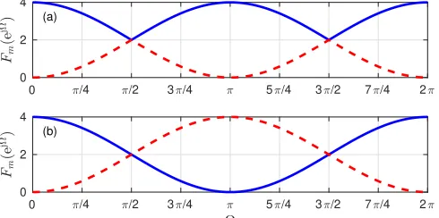
Fig. 1. Selection of (a) spectrally majorised vs (b) analytic functions.

violate analyticity if eigenvalues cross. An example of an an-alytic versus a spectrally majorised solution for the functions

Fm(ejΩ),m = 1,2, is given in Fig. 1. Analytic factors are attractive because they can be approximated by lower order polynomials compared to spectrally majorised ones, with a direct impact on the implementation cost for applications such as broadband beamforming [19–22], angle of arrival estimation [23, 24], or source separation [25].

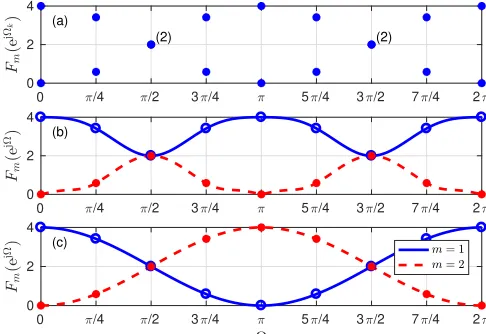
To enforce analyticity over spectral majorisaton in the association across frequency requires a suitable cost func-tion. An example for the arising challenge for the functions in Fig. 1 sampled uniformly atN = 8points in Fig. 2(a) is shown in Figs. 2(b) and (c), where two interpolated curves are woven through a unique and complete assignment of all samples in every frequency bin. Since an analytic function is infinitely differentiable, a smoothness criterion appears to be a good approach to distinguish between the analytic solution and e.g. the spectrally majorised one.

0 /4 /2 3 /4 5 /4 3 /2 7 /4 2 0 2 4 (2) (2) (a)

0 /4 /2 3 /4 5 /4 3 /2 7 /4 2

0 2 4

(b)

0 /4 /2 3 /4 5 /4 3 /2 7 /4 2

0 2 4

(c)

Fig. 2. (a)N = 8sample points obtained from Fig. 1, with (b) spectrally majorised and (c) analytic interpolations.

Below, we investigate the formulation of a cost function based on the infinite differentiability of an analytic function by measuring the power in its derivatives, in order to drive a new set of DFT-based PhEVD algorithms [29].

2. DIRICHLET INTERPOLATION

2.1. Dirichlet Kernel

When describing a 2π-periodic function F(ejΩ) by N eq-uispaced samplesFk = F(ejΩk), Ωk = 2πk/N that have been obtained obeying the Nyquist theorem, the underly-ing interpolation function is the Dirichlet kernel or periodic sinc function, PN(ejΩ). This kernel arises as the discrete-time Fourier transform PN(ejΩ) = PnpN[n]e−jΩn (or shortPN(ejΩ)•—◦pN[n]) of a rectangular windowpN[n]of lengthN, s.t. pN[n] = 1forn=−LN. . .(N−LN−1)and

pN[n] = 0otherwise, whereby we defineLN = (N −1)/2 forNodd, andLN =N/2forNeven.

For the Dirichlet kernelPN(ejΩ), we have, dependent on

Nbeing odd or even:

PN(ejΩ) =

      

sin(N

2Ω) sin(1

2Ω)

=

N−LN−1 P

`=−LN

e−jΩ` _Nodd

e−jΩ2 sin(N

2Ω) sin(1

2Ω)

=

N−LN−1 P

`=−LN

e−jΩ` Neven,

(1)

where the latter expressions in each line are the Fourier series.

2.2. Interpolation

The kernel in (1) permits to express a2π-periodic function

F(ejΩ_)as

F(ejΩ) = 1

N

N−1

X

k=0

FkPN(ej(Ω−Ωk)) (2)

= 1

N

N−1

X

k=0

Fk

N−LN−1 X

`=−LN

e−j(Ω−Ωk)`_{. (3)}

The interpolated expression in (3) can be further simplified to

F(ejΩ) =

N−LN−1 X

`=−LN 1

N

N−1

X

k=0

FkejΩk`e−jΩ`

=

N−LN−1 X

`=−LN

a`e−jΩ` (4)

whereal,l= 0. . .(N−1)are the coefficients resulting from anN-point inverse discrete Fourier transform (DFT) of the sample pointsFk,k= 0. . .(N−1).

3. POWER OF DERIVATIVES BASED ON A COMPLETE SAMPLE SET

We first assume that a functionF(ejΩ_{)is given byN} equi-spaced sampleF(ejΩk_{), Ω}

k = 2πk/N,n = 0. . .(N −1) along the unit circle.

3.1. Power of Derivatives

As a criterion for smoothness, we are interested in the power of thepth derivative ofF(ejΩ_{), which can be measured as}

χp =

1 2π π Z −π dp dΩpF(e

jΩ₎ 2

dΩ, (5)

and can provide a metric for the smoothness ofF(ejΩ_). Dif-ferentiatingF(ejΩ_{)ptimes w.r.t. the frequency parameterΩ} yields

dp dΩpF(e

jΩ_{) =} 1

N N−1 X k=0 Fk dp dΩPPN(e

j(Ω−Ωk)_{) (6)}

=

N−LN1 X

`=−LN

(−j`)pa`e−jΩ` (7)

using (4).

Note that due to orthogonality of the complex exponential terms and integration over an integer number of fundamental periods, for a Fourier series with some arbitrary coefficients

b`, 1 2π π Z −π X l

b`ejΩ`

2

dΩ =X

` 1 2π π Z −π b`ejΩ`

2

dΩ =X

` |b`|2.

Therefore, we can write

χp=

N−LN−1 X

`=−LN

|(−j`)pa`| 2

=

N−LN−1 X

`=−LN

`2p|a`|2. (8)

3.2. Matrix Formulation

Fk along the unit circle and their inverse DFT coefficientsa` organised into vectors,

f = [F0, F1, . . . , FN−1]T (9)

a= [a0, a1, . . . , aN−1]T , (10)

they relate asa= _√1 NT

H

Nf. Further,

D=diag{|−LN|, . . . , 1, 0, 1, . . . (N−Ln−1)}. (11)

Therefore,

χp=aHD2pa=

1

Nf

H_TND2p_TH

Nf . (12)

If power is accumulated across several derivatives up to order

P, then

χ(P)=

P

X

p=0

χp=

1

Nf

H_TN

P

X

p=0

D2pTH_Nf . (13)

This total power can therefore be measures as a weighted in-ner product off,fH_{Cf, with}

C= 1

NTN

P

X

p=0

D2pTH_N . (14)

The matrixD2p_{is positive semi-definite, real, and of rank}

(N−1)forp >0by construction. The inclusion ofD0_into (14) makesCfull rank. With its eigenvalues_N1 PP

p=0D2p, it

condition number isγ=PP

p=0(N−Ln−1)2p, i.e. the matrix becomes ill-conditioned quickly as higher order derivatives are considered.

4. INCOMPLETE SAMPLE SET

If on a regular grid ofN bins, not all sample pointsFk,k =

0. . .(N −1)are available, the idea is to find a maximally smooth interpolation based on an optimum positioning of the missing sample points. Various approaches for this are sug-gested below.

4.1. Schur Complement

It is assumed that on a grid ofN equispaced bins, onlyK < N samples are given. W.l.o.g. these are assumed to be adja-cent1 and are contained ing ∈ CK. We want to select the

remainingN −K coefficient such that maximum smooth-ness is attained for the interpolation. Packed into a vector x∈CN−K, their optimum values can be found as

xopt= arg min x

gHxH

C

g x

. (15)

1_{Otherwise a permutation matrix can be defined, see [32].}

With the partitioning ofCinto

C=

C1 CH2 C2 C4

, (16)

whereC1 ∈ RK×K and all other matrix dimensions as

ap-propriate, we have

xopt=−C−41C2g. (17)

The smoothness metric for the extended vector[gT _xT opt]T can be measured as

χ=gH C1−CH2C −1

4 C2g. (18)

4.2. Minimum Variance Distortionless Response

Based on the relation of the smoothness criterion in (12) to the Fourier coefficients in a ∈ CN, we can formulate the

constrained optimisation problem

min

a a H

P

X

p=0

D2pa s.t. TK_Na=g, (19)

whereTK

N ∈ CK×N containing the appropriateK rows of the N-point DFT TN. The constraint in (19) ensures that the obtained response interpolates through the sample points collected ing∈CK.

The formulation (19) is similar to a minimum variance distortionless response problem, for which Lagrange optimi-sation leads to

aopt=D(P),†TK,NH

TK_ND(P),†TK,_NH −1

g. (20)

Since we are not interested in the coefficientsa_optbut in the smoothness criterionχ, inserting (20) into (19) leads to

χ=gHTKND(P),†T K,H N

−1

g. (21)

5. IMPLEMENTATION AND RESULTS

5.1. Implementation Complexity

To calculate the metric χ for a full set of sample points in f ∈ CN, it is possible to evaluate the matrix C =

TNPP

p=0D 2p_TH

N. The smoothness metric is then given as a weighted inner productχ =fH_{Cf. A computationally} less expense alternative will evaluateTH

Nf as in inverse fast Fourier transform (IFFT) applied tof followed by a vector norm, which results in an overall complexity of

Cfull=N(2 + log2N) (22)

0 0.1 0.2 0.3 0.4 0.5 0.6 0.7 0.8 0.9 1 105

Fig. 3. Complexity of Schur vs MVDR approach.

For a reduced set ofKout of possibleNequispaced sam-ple points, the Schur approach in (18) requires

CSchur= (N−K)3+ (N−K)2K+ (N−K)K2 (23)

MAC operations to calculate theK×Kmatrix that weighs the inner product in (18). This assumes that the diagonal ma-trixP

pD

2p _{is precalculated or available via a look-up}

ta-ble. The major component in (23) is the inversion ofC4 ∈

C(N−K)×(N−K), which is assumed to cost(N−K)3MACs.

For the MVDR method in (21), the cost for constructing the matrix that weighs the inner product is

CMVDR=K3+K2N+KN , (24)

where it is assumed that the inverse of the diagonalP

pD 2p

is available, and that the inversion of theK ×K matrix is accounted byK3_MACs.

Due to the tabling ofP

pD

2p _{and its inverse, the}

com-plexities in (23) and (24) are independent of the orderpof the derivatives, or of the accumulation up to orderP. ForN =

{32,128,512}, the computational costs CSchur andCMVDR are displayed forK= 1. . . Nin Fig. 3. While the MVDR ap-proach inverts a small matrix for smallK, the opposite is true for the Schur approach, where the dimension of the inverse decreases asK →N. Therefore, the MVDR methods offers generally advantages forK < N/2, while forK > N/2the Schur approach becomes preferable.

5.2. Conditioning

Sec. 3.2 stated the full-set matrixCas generally ill-conditioned for largeN andP, even though no matrix inversion is re-quired for the evaluation of the smoothness metric. For the evaluation ofχfor an incomplete sample set however, both Schur and MVDR approaches involve matrix inversions. For the case ofP = 5andN = 32, Fig. 4 shows the condi-tion numbers for the required matrix inversions. Generally, the larger the matrix to be inverted — in the Schur case for small K, in the MVDR case for large K — the worse the conditioning, thus generally necessitating regularisation [30].

0 0.1 0.2 0.3 0.4 0.5 0.6 0.7 0.8 0.9 1

100 105 1010

Fig. 4. Conditioning of Schur vs MVDR approach forN = 32,P = 5, with variableK.

p K= 2 K= 4 K= 7 K= 8 σ2 p 1 0.0270 0.3773 0.4886 0.5000 0.5000 2 0.0564 0.4606 0.4989 0.5000 0.5000 3 0.0689 0.4900 0.4999 0.5000 0.5000 4 0.0722 0.4977 0.5000 0.5000 0.5000 5 0.0730 0.4995 0.5000 0.5000 0.5000

Table 1. Results forχpfor various derivativespand different number of sample pointsK. The power of thepth derivative ofF(ejΩ_),σ2

pis shown for comparison.

5.3. Accuracy

A raised cosineF(ejΩ_{) = 1 + cos Ω, with every derivative} having a power ofσ2

p = 1

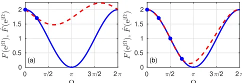
2, is sampled at N = 8 equis-paced bins. The firstK of these sample points are used to evaluate the proposed smoothness metric, with results sum-marised in Tab. 1. For a sufficiently largeK andp, the cor-rect powers are attained. For lower values, an algorithm can find an interpolation with a smaller metric, as demonstrated for{N = 2, p= 4}and{N = 4, p= 2}in Fig. 5.

6. CONCLUSIONS

To measure the smoothness of a function associated with a full or limited set of sample points on the unit circle, this pa-per has suggested the power in the derivatives of the Dirichlet interpolation through the given points. For incomplete sets, also known as the ‘missing samples problem’ [31], a Schur complement and an MVDR approach have been suggested, whereby the latter works best for very sparse sets, while the former operates best on nearly complete sets. Cost, condition-ing and the accuracy of the metric have been explored, with further evaluation and benchmarking left to [32].

0 /2 3 /2 2

0 0.5 1 1.5 2

(a)

0 /2 3 /2 2

0 0.5 1 1.5 2

(b)

Fig. 5. Approximation of raised cosine for (a)N = 2,p= 4

7. REFERENCES

[1] F. Rellich, “St¨orungstheorie der Spektralzerlegung. I. Mit-teilung. Analytische St¨orung der isolierten Punkteigenwerte eines beschr¨ankten Operators,” Mathematische Annalen, vol. 113, pp. DC–DCXIX, 1937.

[2] F. Rellich and J. Berkowitz, Perturbation Theory of Eigen-value Problems, Gordon and Breach, New York, 1969. [3] T. Kato,Perturbation Theory for Linear Operators, Springer,

1980.

[4] B.L.R. De Moor and S.P. Boyd, “Analytic properties of singu-lar values and vectors,” Tech. Rep., KU Leuven, 1989. [5] A. Bunse-Gerstner, R. Byers, V. Mehrmann, and N.K. Nicols,

“Numerical computation of an analytic singular value decom-position of a matrix valued function,” Numer. Math, vol. 60, pp. 1–40, 1991.

[6] K. Wright, “Differential equations for the analytic singular value decomposition of a matrix,” Numerische Mathematik, vol. 63, no. 1, pp. 283–295, Dec. 1992.

[7] L. Dieci and T. Eirola, “On smooth decompositions of matri-ces,”SIAM Journal on Matrix Analysis and Applications, vol. 20, no. 3, pp. 800–819, 1999.

[8] E.S. Van Vleck, Numerical algebra, matrix

the-ory, differential-algebraic equations and control theory: Festschrift in honor of Volker Mehrmann, chapter Continuous Matrix Factorizations, pp. 299–318, Springer, 2015.

[9] P.P. Vaidyanathan, Multirate Systems and Filter Banks, Pren-tice Hall, Englewood Cliffs, 1993.

[10] S. Weiss, J. Pestana, and I.K. Proudler, “On the existence and uniqueness of the eigenvalue decomposition of a parahermi-tian matrix,” IEEE Transactions on Signal Processing, vol. 66, no. 10, pp. 2659–2672, May 2018.

[11] S. Weiss, J. Pestana, I.K. Proudler, and F.K. Coutts, “Cor-rections to on the existence and uniqueness of the eigenvalue decomposition of a parahermitian matrix,”IEEE Transactions on Signal Processing, vol. 66, no. 23, pp. 6325–6327, Dec 2018.

[12] J.G. McWhirter, P.D. Baxter, T. Cooper, S. Redif, and J. Fos-ter, “An EVD Algorithm for Para-Hermitian Polynomial Ma-trices,” IEEE Transactions on Signal Processing, vol. 55, no. 5, pp. 2158–2169, May 2007.

[13] S. Redif, J.G. McWhirter, and S. Weiss, “Design of FIR pa-raunitary filter banks for subband coding using a polynomial eigenvalue decomposition,”IEEE Transactions on Signal Pro-cessing, vol. 59, no. 11, pp. 5253–5264, Nov. 2011.

[14] Z. Wang, J.G. McWhirter, J. Corr, and S. Weiss, “Multiple shift second order sequential best rotation algorithm for poly-nomial matrix EVD,” in23rd European Signal Processing Conference, Nice, France, Sep. 2015, pp. 844–848.

[15] J. Corr, K. Thompson, S. Weiss, J.G. McWhirter, S. Redif, and I.K. Proudler, “Multiple shift maximum element sequential matrix diagonalisation for parahermitian matrices,” inIEEE Workshop on Statistical Signal Processing, Gold Coast, Aus-tralia, June 2014, pp. 312–315.

[16] J. Corr, K. Thompson, S. Weiss, J.G. McWhirter, and I.K. Proudler, “Maximum energy sequential matrix diagonal-isation for parahermitian matrices,” in48th Asilomar Confer-ence on Signals, Systems and Computers, Pacific Grove, CA, USA, Nov. 2014, pp. 470–474.

[17] S. Redif, S. Weiss, and J.G. McWhirter, “Sequential matrix diagonalization algorithms for polynomial EVD of parahermi-tian matrices,” IEEE Transactions on Signal Processing, vol. 63, no. 1, pp. 81–89, Jan. 2015.

[18] J.G. McWhirter and Z. Wang, “A novel insight to the SBR2 algorithm for diagonalising para-hermitian matrices,” in11th IMA Conference on Mathematics in Signal Processing, Birm-ingham, UK, Dec. 2016.

[19] S. Redif, J.G. McWhirter, P.D. Baxter, and T. Cooper, “Ro-bust broadband adaptive beamforming via polynomial eigen-values,” inOCEANS, Boston, MA, Sep. 2006, pp. 1–6. [20] S. Weiss, S. Bendoukha, A. Alzin, F.K. Coutts, I.K. Proudler,

and J.A. Chambers, “MVDR broadband beamforming using polynomial matrix techniques,” in23rd European Signal Pro-cessing Conference, Nice, France, Sep. 2015, pp. 839–843. [21] A. Alzin, F.K. Coutts, J. Corr, S. Weiss, I.K. Proudler, and

J.A. Chambers, “Adaptive broadband beamforming with ar-bitrary array geometry,” inIET/EURASIP Intelligent Signal Processing, London, UK, Dec. 2015.

[22] A. Alzin, F.K. Coutts, J. Corr, S. Weiss, I.K. Proudler, and J.A. Chambers, “Polynomial matrix formulation-based Capon beamformer,” inIMA International Conference on Signal Pro-cessing in Mathematics, Birmingham, UK, Dec. 2016. [23] M. Alrmah, S. Weiss, and S. Lambotharan, “An extension of

the MUSIC algorithm to broadband scenarios using polyno-mial eigenvalue decomposition,” in19th European Signal Pro-cessing Conference, Barcelona, Spain, Aug. 2011, pp. 629– 633.

[24] S. Weiss, M. Alrmah, S. Lambotharan, J.G. McWhirter, and M. Kaveh, “Broadband angle of arrival estimation methods in a polynomial matrix decomposition framework,” inIEEE 5th International Workshop on Computational Advances in Multi-Sensor Adaptive Processing, Dec. 2013, pp. 109–112. [25] S. Redif, S. Weiss, and J.G. McWhirter, “Relevance of

poly-nomial matrix decompositions to broadband blind signal sep-aration,”Signal Processing, vol. 134, pp. 76–86, May 2017. [26] M. Tohidian, H. Amindavar, and A.M. Reza, “A DFT-based

approximate eigenvalue and singular value decomposition of polynomial matrices,”EURASIP Journal on Advances in Sig-nal Processing, vol. 2013, no. 1, pp. 1–16, 2013.

[27] F.K. Coutts, K. Thompson, S. Weiss, and I.K. Proudler, “A comparison of iterative and DFT-based polynomial matrix eigenvalue decompositions,” inIEEE 7th International Work-shop on Computational Advances in Multi-Sensor Adaptive Processing, Curacao, Dec. 2017.

[28] F.K. Coutts, K. Thompson, J. Pestana, I.K. Proudler, and S. Weiss, “Enforcing eigenvector smoothness for a compact DFT-based polynomial eigenvalue decomposition,” in 10th IEEE Workshop on Sensor Array and Multichannel Signal Processing, July 2018, pp. 1–5.

[29] S. Weiss, I.K. Proudler, F.K. Coutts, and J. Pestana, “Iterative approximation of analytic eigenvalues of a parahermitian ma-trix EVD,” inIEEE International Conference on Acoustics, Speech and Signal Processing, Brighton, UK, May 2019. [30] G.H. Golub and C.F. Van Loan, Matrix Computations, John

Hopkins University Press, Baltimore, Maryland, 3rd edition, 1996.

[31] J. Selva, “FFT interpolation from nonuniform samples lying in a regular grid,” IEEE Transactions on Signal Processing, vol. 63, no. 11, pp. 2826–2834, June 2015.

[32] S. Weiss, I.K. Proudler, and M.D. Macleod, “Measuring