High Modularity Creates Scaling
Laws
Peter Grindrod
1& Desmond J. Higham
2Scaling laws have been observed in many natural and engineered systems. Their existence can give useful information about the growth or decay of one quantitative feature in terms of another. For
example, in the field of city analytics, it is has been fruitful to compare some urban attribute, such
as energy usage or wealth creation, with population size. In this work, we use network science and dynamical systems perspectives to explain that the observed scaling laws, and power laws in particular, arise naturally when some feature of a complex system is measured in terms of the system size. Our analysis is based on two key assumptions that may be posed in graph theoretical terms. We assume (a)
that the large interconnection network has a well-defined set of communities and (b) that the attribute under study satisfies a natural continuity-type property. We conclude that precise mechanistic laws are not required in order to explain power law effects in complex systems—very generic network-based
rules can reproduce the behaviors observed in practice. We illustrate our results using Twitter interaction between accounts geolocated to the city of Bristol, UK.
A common theme in recent network science studies has been to partition the vertices of a given graph into mod-ules, also called clusters or communities1, by optimizing a modularity measure2–4. Conceptually, graphs with high
modularity have a dense set of connections between vertices within modules but only sparse connections between vertices within different modules. Thus modularity is usually employed in detecting community structure within large graphs; for example, peer-to-peer friendship and communication graphs often have a high modularity5.
The calculation of a graph’s modularity typically involves some heuristic to search over suitable partitions so as to maximize the chosen modularity measure. Our aim is to reverse this procedure.
Suppose instead that we form a new graph by bringing together a number of separate (disjoint) graphs, each densely connected, as potential modules, and then add a few new edges between nodes from different modules so as to sparsely connect up the whole. Such a modular graph of graphs can form a model of network growth in various applications; see6 for example. Indeed, the widely used stochastic block model7 can be viewed as a
parameter-rich extension to this idea, where edges within and between blocks of nodes are defined with different, independent, probabilities. By considering the growth of such modular graphs as further modules are added, we wish to highlight generic properties of functionals that are well defined over the space of high modularity graphs. In particular we will show that scaling laws arise for well behaved functionals, and that power laws are the dom-inant form of scaling laws.
We believe that this theoretical work adds clarity to the rich and growing literature on empirically observed scaling laws8. For example, focusing on the field of urban analytics, numerous studies have recorded the growth of
some urban indicator, such as wealth, crime rate, walking speed, innovation and energy usage, in terms of popu-lation size9–17. Particular attention has been paid to the distinction between sublinear and superlinear scaling. The
sublinear case has been associated with the efficient use of resources. Analogies have been made between urban growth and other complex systems18–20, and in some cases mechanistic models have been proposed in order to
account for the observed behavior9,21.
Overall, the main contributions of this work are
• to propose a model of network growth based on sparsely connecting a collection of modules
• to impose a realistic assumption that allows us to study functionals of these graphs in terms of the functionals of their underlying modules
• to show that scaling laws arise naturally in this context
1Mathematical Institute, University of Oxford, England, OX2 6GG, UK. 2Department of Mathematics and Statistics, University of Strathclyde, Glasgow, G1 1XH, United Kingdom. Peter Grindrod and Desmond J. Higham contributed equally to this work. Correspondence and requests for materials should be addressed to D.J.H. (email: d.j.higham@ strath.ac.uk)
Received: 5 March 2018 Accepted: 29 May 2018 Published: xx xx xxxx
• to argue that power laws are a natural form of scaling law that, in particular, may be motivated from a dynam-ical systems viewpoint
• to establish that these conclusions apply generically to properties defined by local averaging over vertices, edges or other local substructures
• to show that a generalized model based on random selection of modules produces a result that is sandwiched between scaling laws
• to illustrate the relevance of these conclusions using geolocated social media data.
Methods and Results
Preliminaries.
For any pair of sets, S1 and S2, we denote their disjoint (or discriminated) union byThis indexes the elements in the union according to which of the sets they originated in. The operation obviously extends to one defined on graphs when it is applied to the vertex sets, and consequently any and all edges in the disjoint union of the graphs are inherited directly from the component graphs. Hence the disjoint union of two graphs simply considers them both together, side by side, as a single graph, and is independent of their original indices. A matrix-level description of this operation is summarized in (8).
Let denote the collection of finite undirected graphs with no self-loops and no repeated edges. It is obvi-ously closed under the operation of disjoint union. In particular if S∈ and n∈+, the positive integers, then we will write nS∈ to denote the disjoint union of n isomorphisms of the graph S, that is,
Let Q: → denote a real functional defined over . Then Q(S) measures some property of S which relies on whatever is known about the relationships between its sub-elements (structures), or particular subsets of its sub-elements or vertices. Many graph theoretic properties, including size, average degree, edge density, averaged clustering coefficient, average centrality and various types of modularity measure can be represented by such a Q. We wish to consider properties that are invariant under isomorphisms (re-indexing of the vertices) of S. So a priori the particular indexing of S is irrelevant and there are no distinguishable vertices. We also wish to consider those functionals Q that are effectively continuous with respect to the existence of edges in S, in the sense that if the edge set, E(S), changes by a small amount (relative to the whole) while the vertex set, V(S), remains the same, then Q changes by a correspondingly small amount.
To make this notion precise, let S1 and S2 be graphs on the same set of vertices, with nonempty E(S1) ⊂E(S2). Then let us assume that there exists C>0 such that, for all such S1 and S2 ∈ ,
| − | ≤ | | | | .
Q S Q S C E S S E S
( ) ( ) ( / )
( ) (1)
2 1 2 1
1
Thus the change in Q is linearly bounded by the relative change in the size of the edge set. So if a new fraction ρ of edges are added to S1 then the change in Q is less than Cρ, independently of the choice of S1.
This condition is not satisfied in some immediately obvious cases: for example, if Q counts the number of disjoint connected components then a single additional edge can join two components. Yet the condition holds for properties such as the small world clustering coefficient, the vertex averaged centrality, and various types of modularity. We return to this issue later—see Theorem 1 and its accompanying discussion.
We wish to consider the consequences of condition (1) in the case where we add a few extra edges to nS. We add these edges between the distinct isomorphisms of S, so that the whole, denoted by nS, becomes simply con-nected. This requires approximately n extra connecting edges. So, under (1), for all S we have
|Q nS −Q nS| ≤C n = .
E nS C E S
( ) ( )
( ) ( )
We see that as E(S) become large the change in Q becomes negligible. We may (sparsely) connect up the isomor-phisms of S without changing Q too much.
We emphasize that our overall aim is to study the behavior of a property Q as the network size grows–this cap-tures a regime in which scaling laws are recorded in the experimental literature. Our model for network growth is to add sparse connections to the disjoint union of an increasing number of smaller graphs. This approach is motivated by empirical observations that many real networks have strong modularity. In particular6, showed that
networks of geolocated social media interactions within UK cities can be accurately recreated from individual modules and cities of different sizes are made up of similar modules. We have now shown that if Q satisfies the condition (1), then the model may be simplified further; we may focus our analysis on the disjoint union. On this basis, we are now in a position to introduce and study the concept of a scaling law.
Scaling Functions.
A scaling law is a functional relationship between two physical quantities. In the urban growth context that we highlighted in the introduction, the number of nodes plays the role of population size. The network property Q represents a quantity of interest; for example, in21 this includes measures of energyUsing our model of network growth, we will say that a scaling law exists if there is a scaling function:
× +→
R Z R
G: that describes how the functional Q behaves for disjoint unions of multiple isomorphisms of any set in as follows:
=
Q nS( ) G Q S n( ( ), ), (2)
for all S∈ . Applying G twice, first for n isomorphisms of S and then for m isomorphisms of nS, it is evident that it must satisfy the functional equation
= =
G Q nm( , ) G G Q n m G Q( ( , ), ), ( , 1) Q, (3) for all n and m in + and Q∈+. The identity (3), which is a simple, automatic consequence of a scaling law, will
prove to be extremely useful in our analysis.
Power Law Growth and Decay. We continue by recalling the analysis in [6, Appendix A]. Based on the observa-tion that G(Q, n) =Q/nα satisfies (3), for all α ∈, we consider the ansatz
= α +
G Q n Q
n g n
( , ) ( ),
where g(1) = 0. Suppose that α≠ 0 and g is differentiable, and assume that (3) holds for n and m real. Then directly
= α + .
g nm g n
m g m
( ) ( ) ( )
Differentiating with respect to n and setting n= 1 while g′(1) =αβ for some β ∈, we have αβ
′ = α+ .
g m m
( ) 1
Hence, using g(1) = 0, we obtain g m( )=β
(
1− m1α)
, and thus β= −α+ − −α
G Q n( , ) Qn (1 n ) (4)
is a solution of all α β ∈, , as derived in [6, Equation A.7].
If α is negative (respectively positive) then we obtain power law growth (respectively power law decay to a constant) of the property as the size of the set, measured by n, grows. A value of α different to 1 in (4) corresponds to nonlinear growth, with respect to n.
Now while we might hope that (3) excludes other growth possibilities, and thus explains the ubiquity of power laws observed within many applications, this is simply not so. Consider G(Q, n) =Qn. This is evidently a solution
of (3). However, in the next subsection, we use a dynamical systems viewpoint in order to argue that the asymp-totic power law growth identified in (4) is generic.
The Semigroup Property. Let us relax n to be real and define H(Q, u) =G(Q, eu), for u in . Then (3) implies
+ = = .
H Q u( , v) H H Q u v( ( , ), ), H Q( , 0) Q (5) So (3) is equivalent to this nonlinear semigroup property. Here u (and v) is time -like and moves H along the orbit of an autonomous dynamical system over starting out from Q at time zero. So if F(u|Q) denotes the solution of an autonomous ordinary differential equation, with independent variable u, subject to the initial condition F(0|Q) =Q, then we may set H(Q, u) =F(u|Q) and obtain a solution of (5).
In the linear case where F′=α(β−F) and F(0) =Q, we have H(Q, u) =F(u|Q) =β+ (Q−β)e−uα, implying G(Q, n) =Qn−α+β(1 −n−α), which agrees with the expression derived directly in (4). It is important to note that
this linear case is relevant to a general nonlinear system that has approached a steady state–close to rest points any such qualitative equation is accurately described by its linearization. We therefore argue that the ubiquity of observed (near) power law growth and decay can be associated with the generic local behavior of any linear or nonlinear model that has reached equilibrium.
As an illustration, we note that power law decay applies to the usual modularity measure itself. In6 the
authors derive a lower bound for the modularity of a disjoint union of n graphs, in terms of the modular-ity of the components, each considered in isolation (recall that 1 is always an upper bound for a graph’s modularity). Indexing the component graphs, Sk, by k= 1, ..., n, they obtain the following lower bound on
the modularity of the disjoint union, in terms of the modularities (and thus the partitions) of the separate components:
∑
+∑
− . = = m m R m m m m m F m ( ) 2 (6) k n k k k nk k k
k
1 2 2
Here mk denotes the number of edges in Sk, Rk denotes the modularity of Sk and Fk denotes twice the number
of edges in Sk that connect vertices both lying within the same module (that is, the same element of the optimal
partition of Sk employed in defining Rk). So Fk/2mk is simply the fraction of edges of the kth graph that remain
within a single module.
Now let us define the measure Q so that Q(nS) is the lower bound given by (6) for the modularity of the dis-joint union of n isomorphisms of any S, given that Q(S) is equal to R(k), the actual modularity of S (whence the lower bound is exact). Now applying (6) for a disjoint union of n isomorphisms of a graph, S, where Rk=Q(S),
mk=m/n, and Fk/2mk≡ρ(S), for all k= 1, ..., n, we may define
ρ
= + − .
G Q S n Q S
n S n
( ( ), ) ( ) ( ) 1 1
Here ρ(S) and Q(S) are simply functional properties of the graph S and by construction G(Q(S), n) gives the cor-responding lower bound for the modularity of nS that (i) is a scaling function satisfying (2), and (ii) is of the form anticipated in (4) with α= 1 and β=ρ.
Constraints on the Functional
Q
(
S
).
So far, we have (a) justified a disjoint union network growth model under the assumption (1) on the property of interest and (b) argued that among the collection of scaling laws (2), a power law form is the most natural. In considering the relevance of these observations, it is natural to ask what types of functional, Q(S), admit a scaling law (2). The following result addresses this question by providing a sufficient condition.Theorem 1 Suppose that for all S0 ∈ there existsC S( )0 >0such that Q satisfies
(7) for all S1and S2∈ . Then there exists a scaling function, G, such that (2) must hold for all S in .
Proof. We shall assume (7) together with the converse of (2) and establish a contradiction.
If (2) fails then there must exist a pair of graphs S1 and S2 in and a smallest integer n⁎>1, such that Q(nS1) =Q(nS2) for n= 1, ..., n*− 1, (that is Q cannot distinguish between nS1 and nS2 for n<n⁎) and yet
Q(n*S1) ≠Q(n*S2) (so Q can distinguish between n*S1 and n*S2). Such a situation would make any desired G ill-defined.
On the other hand if Q(S1) =Q(S2) implies Q(nS1) =Q(nS2) for all n≥ 1, and for all S1 and S2 in , then G may be constructed pointwise, at say (Qˆ, n), for all values Qˆ within the range of Q (over ) and all n (by selecting any S for which Q(S) =Qˆ and assigning the corresponding value Q(nS) to G(Qnˆ )).
Now, assume that Q(nS1) =Q(nS2) for n= 1, …, n*− 1 then
Both terms on the right hand side vanish, so Q(n*S
1) =Q(n*S2), giving the required contradiction.
A straightforward corollary to Theorem 1 is that any graph property defined by averaging or summing over some local property belonging to vertices, edges, or other well defined substructures, must have a scaling func-tion. Moreover it must be linear in Q. To see this, let μ(S) denote the total mass in S, over which such an average of some local property is taken. Then
Applying this for i= 1, 2 we have
By Theorem 1 the “total sum” property, Q(S) =μ(S)Q(S), has a scaling function, G say, and
μ( ) ( )nS Q nS =G S Q S n( ( ) ( ), )μ .
μ μ
= .
Q nS G S Q S n S n
( ) ( ( ) ( ), )
( )
But this last must hold for all Q(S) and all μ(S), which might vary independently. Yet the left-hand side is inde-pendent of μ, so G must be linear in its first argument, say G(μ(S)Q(S), n) =h(n)μ(S)Q(S), for some function h(n), and thus
= ≡
Q nS h n Q S
n G Q S n
( ) ( ) ( ) ( ( ), ),
which is linear in Q, as we claimed.
Matrix Function Viewpoint.
Suppose that Q(S) =q(f(M)) is in the form of a real-valued functional, q, of a matrix valued function, f, of either the adjacency matrix, the graph Laplacian matrix, or the normalised graph Laplacian matrix22. We use M to denote any such matrix. If Mi is the corresponding matrix for each Si, i= 0, 1, 2,
then that for is block diagonal:
0 500 1000 1500 2000 2500 0
500
1000
1500
2000
2500
nz = 9076 Bristol adjacency
Figure 1. Adjacency matrix for Bristol network. Dots indicate nonzeros. Node ordering is arbitrary.
0 500 1000 1500 2000 2500 0
500
1000
1500
2000
2500
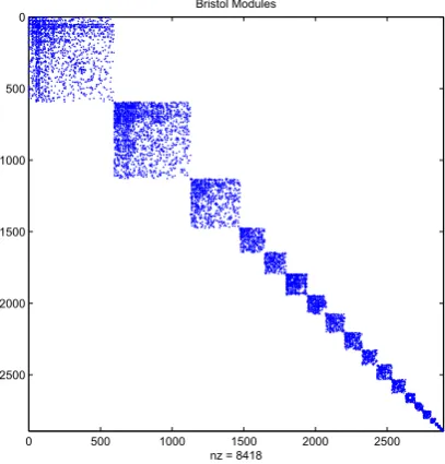
nz = 8418 Bristol Modules
[image:5.595.157.362.47.258.2] [image:5.595.156.360.308.521.2](8) Hence if the f(Mi) are well defined (the spectra of the Mi avoids any singularities and branch cuts for f), then f is
also well defined for the discrete union, and
Then
Now suppose that this last expression is bounded above by
| − | = | − |
C f M q f M( ( )) ( ( )0 1 q f M( ( )2 C f M Q S( ( )) ( )0 1 Q S( ) ,2
for some positive functional C(f(M0)). Then Q has a well defined scaling function G, such that (2) must hold. Simple examples occur when q(f(M)) denotes the sum or the modulus of product of the eigenvalues of f(M) (taking C(M0) to be 1 and |det(M0)| respectively). Now considering the generic properties of matrix valued func-tions23 we see that (if we consider f as subordinate to a complex function) then these last are simply
∑
λ∏
λ= = = = | |
= =
Q S( ) q f M( ( )) f( ) or Q S( ) q f M( ( )) f( ) , i
n i
i n
i
1 1
where the λi denote the eigenvalues of M, and f is any well defined function (meaning well defined at those
eigen-values). Consequently any such Q(S) has a scaling function.
Stochastic Growth and Scaling Laws.
So far we have considered growth when a large network is devel-oped by taking an increasing number of disjoint unions of isomorphic communities, and loosely tying them0 0.5 1 1.5 2
x 104 0
0.5 1 1.5 2 2.5x 10
6
Number of nodes
Graph Measur
e
100 105
101 102 103 104 105 106 107
Number of nodes
Graph Measur
e
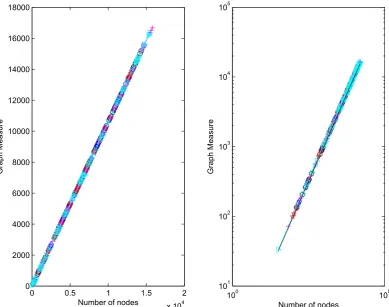
Figure 3. Five independent runs of network growth, showing network size against number of pairs of nodes
[image:6.595.157.549.47.373.2]together. This approach was motivated by the high level of modularity that has been widely observed in real net-works. The simplifying assumption that the communities are isomorphic allowed us to reach precise mathemat-ical conclusions; but in practice we would expect to see modules of different types. In this section, we therefore test our conclusions on a more realistic, stochastic version of the model using real city data. This more general setting is not so amenable to analysis, and hence we give a computational experiment which shows that the same broad conclusions apply.
To set up the stochastic model, let ψ be a probability distribution defined over a finite subset of , that is, those S for which ψ( )S >0 is finite. Then suppose that we draw a sequence of graphs independently and at ran-dom from using ψ, say {S1, S2, …}, and define the cumulative random graphs
Now consider a performance measure Q defined over and satisfying the conditions of Theorem 1. Then Q has a scaling law G such that (2) holds. In the stochastic setting of this section, let qmin= min{Q(S)|S∈ } and qmax = max{Q(S)|S∈ }. Under the reasonable assumption that G(q, n) is monotonically increasing with respect to q, it is clear that
G q( min, )n ≤Q T n( ( ))≤G q( max, ),n n> .1
Hence networks with stochastic growth processes, defined over a finite set of generating networks, are sandwiched between scaling laws. We finish with an experiment on real data that tests the sharpness of these inequalities.
For our computational test, we use a network from6 for the city of Bristol, UK. Figure 1 shows the adjacency
matrix. Here, we have 2892 nodes and 4538 edges. Each node represents a Twitter account that has been geolo-cated to Bristol. An edge between two nodes indicates that the two accounts reciprocally mentioned each other at least once over the period 1–28 October, 2014. In6 this network was also broken down into 20 modules; these
are shown in Fig. 2. This network has the same 2892 nodes, and contains 4209 edges; so the modules capture 93% of the original connections. The module sizes are 593, 536, 345, 172, 149, 147, 133, 129, 122, 104, 103, 95, 68, 54, 54, 32, 19, 16, 11, 10.
To produce Fig. 3, we repeated the same experiment over five independent runs. In each case, we built up a block diagonal matrix by drawing, with replacement, 100 modules. (So in the final network is about 5 times as big as Bristol. This is to show the asymptotic behavior as the network grows.) In other words, we built a block
0 0.5 1 1.5 2
x 104 0
2000 4000 6000 8000 10000 12000 14000 16000 18000
Number of nodes
Graph Measur
e
100 105
101 102 103 104 105
Number of nodes
Graph Measur
e
Figure 4. Five independent runs of network growth, showing network size against sum of Katz centrality
[image:7.595.160.550.46.353.2]diagonal matrix, where the 100 diagonal blocks are drawn randomly from the collection of 20. For k= 1, 2, 3 …, 100 we then add three edges, each edge goes from a randomly chosen node in block k to a randomly chosen node in a different block. Hence, we add 300 new inter-block edges to connect up the network. Then we go through the final adjacency matrix and look at the subnetwork containing all the nodes in block 1, then all the nodes in blocks 1 and 2, then all the nodes in blocks 1, 2 and 3, and so on up to the final case of 100 blocks. So we are growing the network one block at a time, adding a small percentage of random edges. As our first network measure, we choose the number of pairs of nodes that are connected by a path of length five or less. The idea is that a short pathlength-based distance defines a plausible circle of people who might do favors such as find employment opportunities or provide some neighborly domestic support. We chose pathlength five because the individual modules are rich in pairs of nodes connected by shorter paths, and we wished to allow the extra random edges to have some effect. We note that this measure fits into the matrix function framework discussed above. The upper picture in Fig. 3 plots the number of such pairs against the network size. In the lower picture we repeat the same information on a log-log scale, with a reference line of slope 1 added. An underlying staircase effect can be seen, which is caused by the heterogeneity of the modules. A least-squares fit of a power law, log(y) =αlog(x) + con-stant, for each run, produced values of α= 1.3945, 1.2483, 1.2893, 1.3161, 1.4605 over the five runs. Figure 4 gives the corresponding results for the case where the network measure is the sum of components in the Katz centrality vector. We recall5 that with an adjacency matrix B, the Katz centrality vector takes the form (I−aB)−11. Here a is a parameter that must be chosen below the reciprocal of the spectral radius ρ(B). We note that ρ(B) is bounded by the maximum network degree. In our case the maximum observed degree was 54, so we used a= 1/60 through-out. Individual components in this type of centrality measure quantify the importance of network nodes, so the sum can be viewed as an indication of overall effectiveness of the network. In this case we see that the growth is very close to linear; least-squares power law values where 1.0044, 1.0023, 1.0015, 1.0024, 1.0043. Overall, the experiments are consistent with the results derived here, and with the many instances of empirically observed power-law like behavior in the experimental literature.
Discussion
Our aim here was to develop simple, widely applicable, first principle arguments which show that power laws arise generically when some feature of a complex system is measured in terms of system size. The conclusions follow from high-level assumptions concerning the modularity of the underlying networks, the continuity of the network measure of interest and the existence of an underlying, possibly nonlinear, dynamical system describing its growth that has reached equilibrium. Further, the broad conclusions were shown to be robust in an experi-ment where a stochastic version of network growth was used. There are many ways in which these ideas could be pursued, including
• Customized analysis of specific network measures, in particular for the case where the Lipschitz-style condi-tion (1) fails to hold,
• Rigorous analysis of the case of stochastic growth, • Related analysis based on other models of network growth.
References
1. Newman, M. E. J. Communities, modules and large-scale structure in networks. Nature Physics 8, 25–31 (2012).
2. Blondel, V. D., Guillaume, J.-L., Lambiotte, R. & Lefebvre, E. Fast unfolding of communities in large networks. J. Stat. Mech. P10008 (2008).
3. Newman, M. E. J. Modularity and community structure in networks. Proceedings of the National Academy of Sciences 103, 8577–8582 (2006).
4. Newman, M. E. J. & Girvan, M. Finding and evaluating community structure in networks. Phys. Rev. E 69, 026113 (2004). 5. Newman, M. E. J. Networks: an Introduction. (Oxford Univerity Press, Oxford, 2010).
6. Grindrod, P. & Lee, T. E. Comparison of social structures within cities of very different sizes. Royal Society Open Science 3 (2016). 7. Decelle, A., Krzakala, F., Moore, C. & Zdeborová, L. Asymptotic analysis of the stochastic block model for modular networks and its
algorithmic applications. Physical Review E 84, 066106 (2011).
8. Clauset, A., Shalizi, C. R. & Newman, M. E. J. Power-law distributions in empirical data. SIAM Review 51, 661–703 (2009). 9. Arbesman, S., Kleinberg, J. M. & Strogatz, S. H. Superlinear scaling for innovation in cities. Phys. Rev. E 79, 016115 (2009). 10. Bettencourt, L., Lobo, J., Strumsky, D. & West, G. Urban scaling and its deviations: Revealing the structure of wealth, innovation and
crime across cities. PLoS ONE 5, e13541 (2010).
11. Bettencourt, L. & West, G. A unified theory of urban living. Nature 467, 912–913 (2010).
12. Bettencourt, L. M., Lobo, J. & Strumsky, D. Invention in the city: Increasing returns to patenting as a scaling function of metropolitan size. Research Policy 36, 107–120 (2007).
13. DeLong, J. & Burger, O. Socio-economic instability and the scaling of energy use with population size. PLoS ONE 10, e0130547 (2015).
14. Leitão, J. C., Miotto, J. M., Gerlach, M. & Altmann, E. G. Is this scaling nonlinear? Royal Society Open Science 3 (2016).
15. Piovani, D., Zachariadis, V. & Batty, M. Quantifying retail agglomeration using diverse spatial data. Scientific Reports 7, 5451 (2017). 16. Schläpfer, M. et al. The scaling of human interactions with city size. Journal of The Royal Society Interface 11 (2014).
17. van Raan, A. F. J., van der Meulen, G. & Goedhart, W. Urban scaling of cities in the Netherlands. PLoS ONE 11, e0146775 (2016). 18. Batty, M. The New Science of Cities. (The MIT Press, Boston, 2013).
19. Bettencourt, L., Lobo, J., Helbing, D., Kuhnert, C. & West, G. B. Growth, innovation, scaling, and the pace of life in cities. Proceedings of the National Academy of Sciences 104, 7301–7306 (2007).
20. West, G. Scale: The Universal Laws of Life and Death in Organisms, Cities and Companies. (Penguin Press, London, 2017). 21. Bettencourt, L. M. A. The origins of scaling in cities. Science 340, 1438–1441 (2013).
22. Higham, D. J., Kalna, G. & Kibble, M. Spectral clustering and its use in bioinformatics. J. Computational and Applied Math. 204, 25–37 (2007).
Acknowledgements
D.J.H. was supported by EPSRC/RCUK Digital Economy Programme under grants EP/M00158X/1 and EP/ P020720/1.
Author Contributions
P.G. and D.J.H. conceived the experiments, conducted the experiments, analyzed the results and prepared the manuscript.
Additional Information
Competing Interests: The authors declare no competing interests.
Publisher's note: Springer Nature remains neutral with regard to jurisdictional claims in published maps and
institutional affiliations.
Open Access This article is licensed under a Creative Commons Attribution 4.0 International
License, which permits use, sharing, adaptation, distribution and reproduction in any medium or format, as long as you give appropriate credit to the original author(s) and the source, provide a link to the Cre-ative Commons license, and indicate if changes were made. The images or other third party material in this article are included in the article’s Creative Commons license, unless indicated otherwise in a credit line to the material. If material is not included in the article’s Creative Commons license and your intended use is not per-mitted by statutory regulation or exceeds the perper-mitted use, you will need to obtain permission directly from the copyright holder. To view a copy of this license, visit http://creativecommons.org/licenses/by/4.0/.