Reverse sensitivity testing: What does it take to break the model?

City, University of London Institutional Repository

Citation:

This is the submitted version of the paper.

This version of the publication may differ from the final published

version.

Permanent repository link:

Link to published version:

Copyright and reuse: City Research Online aims to make research

outputs of City, University of London available to a wider audience.

Copyright and Moral Rights remain with the author(s) and/or copyright

holders. URLs from City Research Online may be freely distributed and

linked to.

City Research Online: http://openaccess.city.ac.uk/ [email protected]

What does it take to break the model?

Silvana M. Pesenti∗1_{, Pietro Millossovich}1,2_{, and Andreas Tsanakas}1 1_{Cass Business School, City, University of London}

2_{DEAMS, University of Trieste}

January 23, 2018†

Abstract

Sensitivity analysis is an important component of model building, interpretation and validation. A model comprises a vector of random input factors, an aggrega-tion funcaggrega-tion mapping input factors to a random output, and a (baseline) probability measure. A risk measure, such as Value-at-Risk and Expected Shortfall, maps the distribution of the output to the real line. As is common in risk management, the value of the risk measure applied to the output is a decision variable. Therefore, it is of interest to associate a critical increase in the risk measure to specific input factors. We propose a global and model-independent framework, termed ‘reverse sensitivity testing’, comprising three steps: (a) an output stress is specified, corresponding to an increase in the risk measure(s); (b) a (stressed) probability measure is derived, minimising the Kullback-Leibler divergence with respect to the baseline probability, under constraints generated by the output stress; (c) changes in the distributions of input factors are evaluated. We argue that a substantial change in the distribution of an input factor corresponds to high sensitivity to that input and introduce a novel sensitivity measure to formalise this insight. Implementation of reverse sensitivity testing in a Monte-Carlo setting can be performed on a single set of input/output scenarios, simulated under the baseline model. Thus the approach circumvents the need for additional computationally expensive evaluations of the aggregation func-tion. We illustrate the proposed approach through a numerical example of a simple insurance portfolio and a model of a London Insurance Market portfolio used in in-dustry.

KeywordsRobustness and sensitivity analysis, risk management, Value-at-Risk, Ex-pected Shortfall, stress testing.

1

Introduction

1.1 Problem framing and contribution

Risk managers often use complex quantitative models as decision support tools. Sensi-tivity analysis is concerned with characterising and providing insight regarding the rela-tion between inputs and outputs. Sensitivity analysis can have different aims, including

∗

Corresponding author. Email: [email protected]

†

identifying the most or least influential inputs (factor prioritisation or factor fixing re-spectively), detecting the direction of input/output relationships, and inferring model structure; see Saltelli et al. (2008); Borgonovo and Plischke (2016) for comprehensive reviews.

For the specific aim of factor prioritisation, a sensitivity measure is typically used, assigning a sensitivity score to each input. When model inputs are subject to uncertainty,

global sensitivity measures are used, considering the whole possible space of multivariate input scenarios. Such methods typically involve a comparison of the unconditional and conditional output distributions, when individual inputs are fixed, see Borgonovo et al.

(2016) for a unifying framework. Prominent methods use a (Hoeffding) decomposition of the output variance (Saltelli et al., 2000; Saltelli, 2002; Saltelli et al., 2008), as well as moment independent approaches (Borgonovo,2007;Borgonovo et al.,2011). Alternative methods consider partial derivatives of statistical functionals of the output distribution in the direction of parameters of interest, seeGlasserman and Liu(2010) for expectation-type andHong (2009);Tsanakas and Millossovich(2016) for percentile-based functionals.

In this paper we develop a sensitivity analysis framework appropriate for contexts where the following considerations, typical in several fields, including probabilistic safety assessment, reliability analysis and financial/insurance risk management (Saltelli and Tarantola, 2002; Aven and Nøkland, 2010; Gourieroux et al., 2000; Tsanakas and Mil-lossovich,2016), hold:

• Model inputs are uncertain, hence sensitivity and uncertainty analyses are inter-linked and global sensitivity analysis methods are called for.

• A decision criterion is derived by applying arisk measure on the distribution of the output. Risk measures are functionals mapping random variables to the real line (Artzner et al.,1999;Szeg¨o,2005). Risk measures are used in a variety of operations research and risk analysis applications, with Value-at-Risk (VaR) and Expected Shortfall (ES – also known as CVaR) particularly popular choices; indicatively see

Rockafellar and Uryasev(2002);Tapiero(2005);Gotoh and Takano(2007);Ahmed et al.(2007); Asimit et al.(2017).

• The value of the risk measure, applied on the output distribution, gives an indication of criticality for the system whose uncertainty is analysed. For example, in the context of financial risk management, high values of output risk measures may indicate that a portfolio is not admissible, e.g. due to regulatory constraints (Artzner et al.,1999). In the context of probabilistic safety assessment, legislation postulates acceptable probabilities of failure, e.g. of fatality numbers exceeding a threshold (Borgonovo and Cillo,2017). Hence it is of interest to identify which inputs would be influential in a change of the model that leads to an unacceptable increase in the value of the output risk measure.

• The relationship between model inputs and outputs is complex and not necessarily given in analytical form; furthermore, evaluations of the model are computationally expensive. Therefore, it should be possible to estimate sensitivity measures from a single sample of input and output scenarios (Plischke et al.,2013).

We propose a sensitivity analysis framework, adapted to the above context, termed

reverse sensitivity testing. We work in the standard setting of sensitivity analysis, where a number of random input factors are mapped to a random output via an aggregation

output in current specification of the model. Reverse sensitivity testing comprises the following steps. First, an output stress is defined, corresponding to an increase in the value of the output risk measure. We focus on the widely used risk measures VaR and ES. The increase in the value of the risk measure is specified so as to produce a stress that is problematic to a decision maker. For example, in a capital management context, a stress on VaR may lead to a situation where insufficient assets are available to satisfy regulatory requirements.

Secondly, a stressed probability measure is derived. This is a probability (a) under which the risk measure applied to the model output is at its stressed level and (b) that minimises the Kullback-Leibler (KL) divergence subject to appropriate constraints on the output probability distribution. Thus the stressed probability leads to the most plausible alternative model, under which the output distribution is subjected to the required stress. We derive analytical solutions of the stressed probability measure under an increase of VaR and ES. The form of the solutions allows for numerically efficient implementation via a single set of Monte-Carlo simulations.

Finally, the distribution of individual input factors is examined under the baseline and stressed models. Substantial changes in the distribution of a particular input indicate a large sensitivity to that input. A new class ofreverse sensitivity measures is introduced, quantifying these input changes. The sensitivity measures are then used to identify the most influential input factors; in a sense, those factors that may be responsible for ‘break-ing the model’.

1.2 Relation to the literature

The sensitivity measures we derive ultimately reflect the joint distribution of individual input factors and output; hence our proposed method remains formally within the uni-fying framework discussed byBorgonovo et al. (2016) and thus are (distantly) related to variance-based (Saltelli et al.,2008) and moment-independent (Borgonovo,2007) sensitiv-ity measures. Conceptually, the reverse direction (from output to input) of the proposed method, is related to regionalised sensitivity analysis methods (Spear et al., 1994; Os-idele and Beck,2004). However, there is a key difference between regionalised sensitivity analysis and our approach: in the former, states of the output are identified that are ‘out of control’, while in the latter what is ‘out-of-control’ are not individual states but specifications of the output distribution.

In the practice of financial risk management and regulation, reverse stress testing, starting with a stressed output state and studying the corresponding surface of scenarios that provide the adverse outcome, is frequently used (BCBS, 2013; EIOPA, 2009). For example, “reverse stresses that result in a depletion of capital...” (Lloyd’s,2016) are used in the validation of insurance risk models. The academic literature on reverse stress testing is relatively sparse, with a recent focus towards identifying most likely stress scenarios (McNeil and Smith,2012;Breuer et al.,2012;Glasserman and Xu,2014). Once again, our approach differs from reverse stress testing, in that we consider most influential factors in relation to changes in the output distribution and not a particular output state.

The KL-divergence has been widely used in financial risk management, in particular in the context of model uncertainty, where several plausible specifications of the probability measure may co-exist. For example, Breuer and Csisz´ar (2013); Glasserman and Xu

minimal KL-divergence that satisfies given constraints. Our approach is closely related to the work of Cambou and Filipovi´c (2017) with probability set constraints and Weber

(2007) with risk measure constraints. In this paper, we provide additional risk measure constraints not studied in those papers and generalise some results of Weber (2007) by dropping the assumption of bounded random variables.

1.3 Structure of the paper

In Section 2, some preliminaries on risk measures and the KL-divergence are given. In Section3, the optimisation problem yielding stressed probability measures is stated and solved under constraints arising from different risk measures, with emphasis on VaR and ES. Explicit solutions allow easy implementation and inspection of the distributional changes arising. The solutions and their properties are illustrated through an example of a non-linear insurance portfolio evaluated using Monte-Carlo simulation.

Section 4 is devoted to a comparison of the stressed and the baseline probability measures through stochastic order relations. The output under the baseline probability is first-order stochastically dominated by the stressed probability. A similar dominance relation is given for input factors, under the assumption of a non-decreasing aggregation function and positive dependence between input factors. Moreover, stressed probability measures stemming from different stress severities lead to stochastically ordered input factors and output.

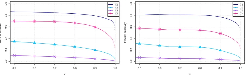
In Section5 we propose two sensitivity measures specifically tailored to the proposed reverse sensitivity testing approach. A reverse sensitivity measure quantifies the extent that the distribution of an input factor is distorted by the transition to a stressed prob-ability. A forward sensitivity measure is an associated metric that considers the change in output from stressing a particular input. These sensitivity measures can be viewed as dependence metrics between individual input factors and the output. We conclude with an application of the reverse sensitivity testing framework to a commercially used insurance portfolio risk model.

2

Preliminaries

We consider a measurable space (Ω,A) and denote byP the set of all probability measures on (Ω,A). For a random variable Z on (Ω,A) we write F_ZQ(·) = Q(Z ≤ ·) for its distribution under Q ∈ P, and similarly, EQ(·) for its expectation. Throughout, we use the Kullback-Leibler divergence (KL-divergence, Kullback and Leibler (1951)) as a measure of discrepancy between two probability measures. For Q1, Q2 ∈ P, the KL-divergence, also known as relative entropy, ofQ1 with respect toQ2 is defined by

DKL(Q1kQ2) =

(R dQ1

dQ2log

dQ1

dQ2

dQ2 ifQ1 Q2

+∞ otherwise.

The KL-divergence is non-negative, vanishes if and only ifQ1 ≡Q2, and is in general not symmetric (Kullback, 1997; Cover and Thomas, 2012). The KL-divergence is a special case of the class off-divergences, first introduced byAli and Silvey(1966), for the choice

f(x) =xlog(x), x >0. For a given convex functionf, thef-divergence ofQ1with respect toQ2, for anyQ1, Q2∈ P, is defined throughDf(Q1kQ2) =

R

f dQ_dQ12

dQ2 .

a overview. Moments, such as the mean and standard deviation, can be seen as risk measures. In recent years, percentile-based risk measures (Acerbi, 2002) have become prominent, with the most commonly used risk measures being Value-at-Risk (VaR) and Expected Shortfall (ES). These risk measures are used extensively in financial regula-tion for the calcularegula-tion of capital requirements, specifically VaR for European insurance companies,EIOPA (2009), and ES for banks,BCBS (2012,2013).

The VaR at levelα∈[0,1] of a random variableZ is defined as the leftα-quantile of the distribution ofZ, VaRQ_α(Z) =F_ZQ,−1(α) = inf{z ∈_R|F_ZQ(z) ≥α}, where, as usual, inf∅= +∞. In particular, the essential supremum of Z is ess supQZ =F_ZQ,−1(1). The

ES (also CVaR) ofZ at levelα∈[0,1) is defined by

ESQ_α(Z) = 1 1−α

Z 1

α

VaRQ_u(Z)du= 1 1−αE

Q _Z−VaRQ α(Z)

+

+ VaRQ_α(Z),

where, in the second representation, VaRQ_α(Z) can be replaced by any α-quantile ofF_ZQ. Unlike VaR, the ES takes into account the whole tail of the distribution ofZ, that is all realisations larger than VaRQ_α(Z). SeeF¨ollmer and Schied(2011) for a comparison of the two risk measures.

Shortfall risk measures, associated with utility-type arguments, are defined through

ρQ(Z) = inf{z ∈ _R|EQ(`(Z −z)) ≤ z0} for Q ∈ P, where ` is a decreasing, non-constant and convex loss function while z0 is a point in the interior of the range of ` (F¨ollmer and Schied, 2002). Examples of shortfall risk measures include entropic risk measures, Gerber(1974), and the class of generalised quantiles called expectiles (Newey and Powell,1987;Bellini et al.,2014).

3

Deriving the stressed model

3.1 Problem statement

We consider the standard setting of (reverse) sensitivity analysis, involving a (typically complicate) function, mapping model inputs to an output that is used in a decision making process. Mathematically, we define the input factors as a random vector X = (X1, . . . , Xn) on the measurable space (Ω,A). The (measurable) function g:Rn → R,

is called the aggregation function, which gives, when applied to input factors X the one-dimensional randomoutput of interest Y = g(X). The variability of the output Y

to changes in input factors is of fundamental importance in sensitivity analysis (Saltelli et al., 2008; Borgonovo and Plischke, 2016). We adopt throughout the convention that large values of the output correspond to adverse states.

We call the triple (X, g, P), the baseline model with baseline probability measure

P ∈ P. The probability P is seen as encoding current beliefs regarding (or software implementation of) the distribution ofX. Under the baseline probabilityP we suppress the superscript and write, for example,FZ(·) =FZP(·) andE(·) =EP(·), and analogously for risk measures, VaRα(·) = VaRPα(·) and ESα(·) = ESPα(·). We call any Q ∈ P an

alternative probability measure and (X, g, Q) an alternative model. A Radon-Nikodym (RN) density is a non-negative random variable ζ on (Ω,A) such that E(ζ) = 1. We denote byQζ _{the probability measure which is absolutely continuous with respect to P} with RN-densityζ, that is, ζ = d_dQ_Pζ.

representing system failure, increases to an extent that the risk of failure is no longer ac-ceptable. Specific stress definitions using different risk measures are discussed in Sections

3.2-3.5. Subsequently, we call (X, g, Q) astressed model withstressed probability measure

Q∈ P if, underQ, the outputY fulfils a set of probabilistic constraints (the stress) and

Qhas minimal KL-divergence with respect toP. Thus, a stressed probability measure is defined as a solution to

min

Q∈PDKL(QkP), s.t. constraints on the distribution of Y under Q. (1)

The optimisation problem (1) is robust in the sense that convergence in the KL-divergence implies weak convergence of the

probability measures, Gibbs and Su (2002). This means that an alternative proba-bility which satisfies the constraints of (1) and is close in KL-divergence to the stressed probability, is also close to the stressed probability in the L´evy metric.

Optimisation problem (1) under linear (i.e. moment) constraints was first studied in the seminal paper by Csisz´ar (1975). In the context of financial risk management, in particular when risk measures are used, optimisation problem (1) involves non-linear constraints and Csisz´ar’s theory cannot be applied. Relevant research includes Cambou and Filipovi´c (2017) who consider the optimisation problem for general f-divergences and probability set constraints. Weber(2007) works with bounded random variables and considers risk measure constraints such as ES and shortfall risk measures, see Sections

3.3and 3.4 for a more detailed comparison. The related problem of finding a worst-case distribution with respect to alternative probabilities lying within a KL-divergence distance of the baseline probability is addressed inBreuer and Csisz´ar(2013) andGlasserman and Xu(2014) and Blanchet et al.(2017). We refer toBen-Tal et al. (2013) for robust linear optimisation with generalf-divergence constraints.

3.2 Probability constraints

Before studying problem (1) with constraints involving the risk measures of Section 2, we consider stresses under which the probabilities of (adverse) outcomes of Y = g(X) are altered. These outcomes are captured by disjoint sets B1, . . . , BI ⊆ R, each set Bi associated with an event {Y ∈ Bi} where the system being studied is failing or ‘out of control’. In a financial context, whereY is interpreted as a loss, one can identifyBi with a region of extreme losses.

The following result is an immediate consequence of Theorem 3.1 in Csisz´ar(1975); we also refer toCambou and Filipovi´c (2017).

Proposition 3.1. Let B1, . . . , BI ⊆R be disjoint Borel sets withP(Y ∈ Bi) > 0, i = 1, . . . , I, and α1, . . . , αI > 0 such that α1 +· · ·+αI ≤ 1. Then there exists a unique solution to

min

Q∈PDKL(QkP), s.t. Q(Y ∈Bi) =αi, i= 1, . . . , I, (2)

with RN-density given by ζ = PI

i=0 αi

P(Y∈Bi)1{Y∈Bi}, where we write α0 = 1−

PI

i=1αi andB0= (SI_i=1Bi)c.

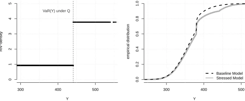
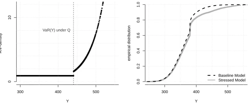
3.3 VaR constraints

We now consider optimisation problem (1) under a constraint on the risk measure VaR, applied to the outputY. A VaR constraint is not equivalent to a probability constraint of optimisation problem (2), whenFY is not strictly increasing.

Proposition 3.2. Let 0 < α < 1 and q ∈ _R such that VaRα(Y) < q < ess supY and consider the optimisation problem

min

QPDKL(QkP), s.t. VaR

Q

α(Y) =q. (3)

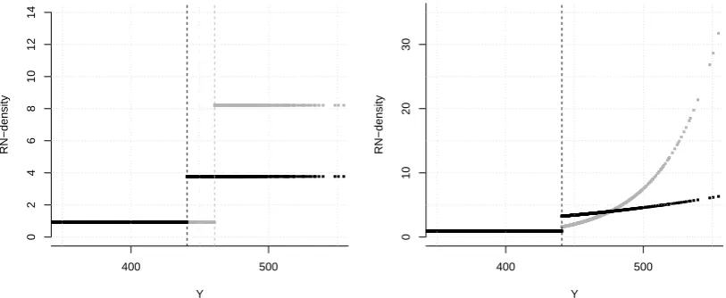
There exists a unique solution to (3) if and only if P(q−ε < Y < q) >0 for all ε > 0. The RN-density of the solution is given by

ζ = α

P(Y < q)1{Y <q}+

1−α

P(Y ≥q)1{Y≥q}.

The assumption P(q−ε < Y < q)>0 for all ε >0, implies that q cannot be chosen arbitrarily. In particular, problem (3) does not have a solution, if the distribution of Y

is constant to the left of q (q excluded); this includes the (uncommon in practice) case whereY is a discrete random variable. This complication arises from using the constraint VaRQ_α(Y) =q rather than Q(Y ≤q) =α. Ifq cannot be chosen to fulfil the assumptions in Proposition 3.2, the form of ζ in Proposition 3.2 remains meaningful: by Proposition

3.1, it is the solution to an optimisation problem where the constraint VaRQ_α(Y) =q is replaced byQ(Y < q) =α.

The RN-density ζ of the solution to (3) is a non-decreasing function of Y since α ≤ P(Y ≤VaRα(Y))≤P(Y < q). Hence, under the stressed probability, adverse realisations of the output are given higher probabilities of occurrence. This is now demonstrated by an example taken from insurance risk modelling.

Remark. Propositions3.1and 3.2hold true for any f-divergence with a strictly convex function f. In particular, the RN-densities ζ of the solutions are independent of the choice of f-divergence. We do not provide a proof for this statement, however the steps of the proofs of Propositions 3.1 and 3.2 can be closely retraced if one substitutes the KL-divergence with a generalf-divergence.

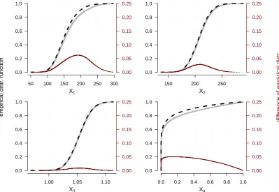
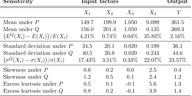
Example. The following insurance portfolio, similar to Example 1 inTsanakas and Mil-lossovich(2016), will be used as an illustrative example throughout the paper. An insur-ance company faces a loss Lresulting from two lines of business. The two lines produce losses X1, X2 respectively, which are subject to the same multiplicative inflation factor

X3, such that L = X3(X1 +X2). The insurance company has a reinsurance contract on the loss L with limit l and deductible d. The total portfolio loss for the insurance company is

Y =L−(1−X4) min{(L−d)+, l},