City, University of London Institutional Repository
Citation
:
Jones, P. R. ORCID: 0000-0001-7672-8397, Landin, L., McLean, A., Juni, M. Z., Maloney, L. T., Nardini, M. and Dekker, T. M. (2019). Efficient visual information sampling develops late in childhood. Journal of Experimental Psychology: General, 148(7), pp. 1138-1152. doi: 10.1037/xge0000629This is the accepted version of the paper.
This version of the publication may differ from the final published
version.
Permanent repository link:
http://openaccess.city.ac.uk/22420/Link to published version
:
http://dx.doi.org/10.1037/xge0000629Copyright and reuse:
City Research Online aims to make research
outputs of City, University of London available to a wider audience.
Copyright and Moral Rights remain with the author(s) and/or copyright
holders. URLs from City Research Online may be freely distributed and
linked to.
City Research Online: http://openaccess.city.ac.uk/ [email protected]
In press, JEP:General (April 2019)
Efficient visual information sampling develops late in childhood
Peter R. Jones1,2, Linnea Landin3, Aisha McLean1, Mordechai Z. Juni4,
Laurence T. Maloney5,6, Marko Nardini*,7, Tessa M. Dekker*,Ŧ,1,3
1 Institute of Ophthalmology, University College London (UCL), London, UK.
2 NIHR Moorfields Biomedical Research Centre, London, UK
3 Division of Psychology and Language Sciences, University College London (UCL), London, UK. 4 Department of Psychological and Brain Sciences, University of California, Santa Barbara, USA 5 Department of Psychology, New York University, New York, USA
6 Center for Neural Science, New York University, New York, USA 7 Department of Psychology, Durham University, Durham, UK.
Abstract
It is often unclear which course of action gives the best outcome. We can reduce this uncertainty by gathering more information; but gathering information always comes at a cost. For example, a sports player waiting too long to judge a ball’s trajectory will run out of time to intercept it. Efficient samplers must therefore optimize a trade-off: when the costs of collecting further information exceed the expected benefits, they should stop sampling and start acting. In visually guided tasks, adults can make these trade-offs efficiently, correctly balancing any reductions in visuomotor uncertainty against cost factors associated with increased sampling. To investigate how this ability develops during childhood, we tested 6-11 year-olds, adolescents, and adults on a visual localization task in which the costs and benefits of sampling were formalized in a quantitative framework. This allowed us to compare participants to each other, and to an ideal observer who maximizes expected reward. Visual sampling became
substantially more efficient between 6-11 years, converging onto adult performance in adolescence. Younger children systematically under-sampled information relative to the ideal observer and varied their sampling strategy more. Further analyses suggested that young children used a suboptimal decision rule that insufficiently accounted for the chance of task failure, in line with a late developing ability to compute with probabilities and costs. We therefore propose that late development of efficient
information sampling, a crucial element of real-world decision-making under risk, may form an important component of sub-optimality in child perception, action, and
decision-making.
Introduction
Everyday actions can have uncertain outcomes. We may try to catch a ball but have only partial information about its trajectory. Accumulating more information before acting can help reduce this uncertainty, increasing the chance of success. But because information typically comes at a cost, we must often decide whether to gather more information or act on what we already have.
For example, when crossing a busy road, we may pause to estimate the speeds and trajectories of oncoming traffic before deciding when to cross. If we gather too little information, we dart into traffic risking an unnecessary disaster. Gathering too much information, however, carries its own costs as we find ourselves standing beside the road indefinitely, missing gaps in traffic we might have crossed. Changes in the costs of waiting or the benefit of information, lead to changes in the behaviour that maximise expected utility. Late for a meeting, we are more likely to rush into traffic, accepting slightly higher risks in return for a timely arrival. On foggy days we may sensibly look more carefully before stepping into traffic.
Similarly, a goalkeeper defending a penalty kick may leap too soon and end up on the wrong side of the net, or observe the striker for too long and leap in the correct direction, but have insufficient time to stop the ball. So, while looking reduces the keeper’s visual uncertainty, it comes at a cost of motor precision. Since looking too long or too little will result in more failed saves in the long run, a quality keeper should maximise save-rate by finding the ideal trade-off that balances sampling costs and benefits.
Such decisions require an assessment of how well one might do with and without additional information, and of whether the cost of gathering more information is worth the benefit. This is fundamental to all tasks in which information gathering can reduce uncertainty about succeeding, and includes not just perception-guided actions such as navigating traffic or playing sports, but also more cognitive tasks such as deciding how long to study for a test or look around before purchasing a house. Here we investigate how and when this fundamental information gathering skill develops between childhood and adulthood.
probabilities of each possible event (explore), or bet on which event would occur next to win points - but without feedback (exploit). Human performance was markedly sub-optimal: participants sampled 8 to 9 times the amount of information needed to maximize their expected winnings. Busemeyer & Rapoport (1988), using a similar costly sampling task, found that participants considered costs and benefits of sampling when deciding when to stop, but in some cases also sampled more than they should have to maximize their score.
Contrasting behavior is found in “secretary problems” (Ferguson, 1989) and similar tasks, in which adults see a sequence of items differing in value and can either select the current item or go on to the next – they cannot go back to a previously rejected item. In these tasks, participants tend to stop too soon, lowering their chance to maximize winnings (Bearden, Rapoport, & Murphy, 2006; Kahan, Rapoport, & Jones, 1967; Rapoport & Tversky, 1970; Seale & Rapoport, 1997).
Thus, in cognitive sampling tasks with clearly defined optimal strategies, adults often fail to follow this optimal strategy and maximize expected gain. In more recent free sampling tasks, adults see two lotteries, (e.g., decks of cards with varying points and penalties) from which they can freely sample to identify the more profitable lottery (Hertwig, Barron, Weber, & Erev, 2004). Participants typically sample only a few times (~15-20) before choosing which lottery to play. This has been characterized as under-sampling (Hau, Pleskac, Kiefer, & Hertwig, 2008), but without quantified sampling costs, it is unclear what the gain-maximizing stopping rule is (Juni, Gureckis, & Maloney, 2016).
It has been argued that adults in cognitive sampling tasks may be using a more adaptive strategy than first appears. For example, under-sampling may in fact reflect optimal stopping giving intrinsic costs such as boredom, fatigue, or different value assigned to payoff (Dudey & Todd, 2001; Seale & Rapoport, 1997). Participants might also be sampling optimally within the constraints of limited memory or planning capacity (Busemeyer & Rapoport, 1988; Hertwig et al., 2004; Rakow, Demes, & Newell, 2008; Rakow & Rahim, 2010), or base their stopping rules on heuristics, that whilst suboptimal, are reasonably successful at identifying the ideal strategy (Evans and Buehner, 2011; Fiedler and Kareev, 2011; Hertwig and Pleskac, 2010).
Maloney, 2007; Faisal & Wolpert, 2009; Juni et al., 2016). Typically, these tasks have a strong emphasis on ideal observer models that capture the costs and benefits of visual information sampling, and that test participants’ abilities to balance these factors to maximize expected gain. In Battaglia & Schrater (2007) for example, the observer can delay his response in order to acquire more information about the location of a visual target but this comes at the cost of movement time - and hence precision - to hit the target and earn a reward. The typical finding in these tasks is that without much task-specific training, participants are able to trade off the benefit of further sampling against its costs to maximize their winnings. This suggests that in visuomotor tasks, adults are highly adept at estimating and accounting for their own visual sampling skills, and make complex sampling choices with surprising speed and automaticity.
Like adults, children also face many tasks that rely on the ability to decide when to stop looking and start acting. In everyday risky activities such as crossing the road or playing outside, inefficient sampling choices could have a major impact on childhood safety. However, as yet, little is known about the contributions of this crucial decision-making skill to visuomotor development. In one recent developmental study, children and teenagers’ decisions from sampling were investigated in the
cognitive domain, using a classic card-sampling paradigm. The results revealed that 8 year-olds sampled approximately the same numbers of cards as adults to learn the payoffs of two lotteries before selecting one to play for points. In contrast, adolescents between the ages of 12-14 years sampled significantly less information than children or adults before playing, revealing a U-shaped developmental trajectory. Based on correlations with questionnaire data, the authors hypothesized that the age differences were linked to reduced motivation in the teenage years (Van den Bos & Hertwig, 2017). However, to date, it is unclear how sampling decisions develop in a visuomotor context when the payoff structure derives from a noisy visual estimate – even though this is a type of sampling problem young children face very frequently in everyday life, and that has major implications for physical safety.
proportion to its reliability (Ernst, 2012; Ernst & Banks, 2002). In contrast, across a range of tasks and cue combinations children only start weighting cues by their precisions after the age of 10-11 years, keeping cues separate before this time (Gori, Del Viva, Sandini, & Burr, 2008; Nardini, Bedford, & Mareschal, 2010; Nardini, Jones, Bedford, & Braddick, 2008).
One recent study suggests that the ability to weight the rewards and penalties of different visuomotor action outcomes by their likelihoods also poses a challenge for children up to the age of 11 years (Dekker & Nardini, 2016). When making rapid reaches to a display with reward and penalty regions, adults correctly accounted for the imprecision of their reaches, and aimed for locations that would nearly maximize their expected score (Trommershäuser, Maloney, & Landy, 2003). Children, in contrast, aimed for “risky” regions with a high chance of winning but also a high risk of loss, to the detriment of their expected score. Interestingly, a similar preference for “risky” lotteries with high outcome variability has often been reported in childhood and adolescence for gambles with explicitly stated probabilities and values (Boyer, 2006; Defoe, Dubas, Figner, & van Aken, 2015; Levin, Hart, Weller, & Harshman, 2007; Steinberg, 2008; Weller, Levin, & Denburg, 2011), although it is unclear whether similar factors may underlie both types of decisions.
In any case, adults typically perform close to ideal on sensorimotor decision-tasks. In contrast, in children younger than ~10 years old, the available sensorimotor information is not combined and weighted correctly, leading to substantially poorer perceptual performance than that of an ideal observer (Gori, Del Viva, Sandini, & Burr, 2008; Nardini, Bedford, & Mareschal, 2010; Nardini, Jones, Bedford, & Braddick, 2008). Similarly, in a rewarded setting, this phenomenon with children led to substantially lower winnings compared to a gain-maximizing observer under the same conditions (Dekker & Nardini, 2016). Therefore, we hypothesized that younger children will also make inefficient sampling choices when the costs and benefits of sampling are determined by their own visual abilities, and that this ability will improve with age.
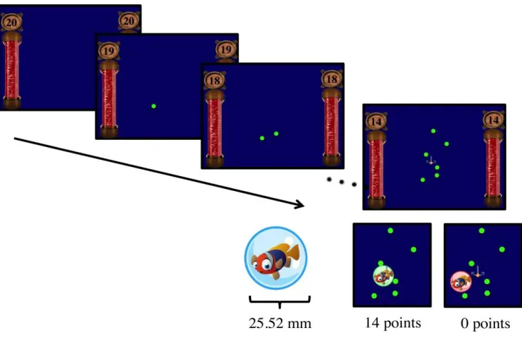
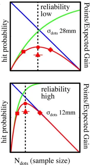
During the experiment, we asked 6 to 12-year-olds, 13 to 15-year-olds, and adults, to locate a hidden target (a cartoon fish) by pressing on a touchscreen. To locate the fish, participant could ‘buy’ cues to the target location, but in doing so the potential reward was reduced. Each cue was a bubble (marked as a green dot) that appeared on the screen (Figure 1). Each dot was drawn from an isotropic bivariate Gaussian (Normal) distribution centred on the target. The more dots observed (i.e., sampled), the more likely it became that the centroid of the observed dots lay within the target containing the fish. The probability of catching the fish thus increases with each additional dot observed. However, each additional dot reduced the potential reward (green curve and blue line, Figure 2). The expected reward for any number of dots is the product of the reward for the fish and the probability of catching it (red curve, Figure 2). The ideal observer would sample the number of dots with the highest expected reward (dashed line, Figure 2).
Thus, as in everyday sampling problems (e.g., deciding when to cross a road), minimising risk involves estimating the benefits of additional information gathering as defined implicitly by noise in the visual estimate, and then trading this information off against the sampling cost. As in naturalistic sampling, observers must select the best trade-off from a range of potential sampling strategies with different expected payoffs.
Juni et al (2016) found that adult participants performed this task in qualitative agreement with the optimal strategy, buying fewer location cues when the cost of each cue increased. In one of their experimental conditions (low stakes), there was no patterned deviation in sampling from the ideal; though in a second condition (high stakes), participants sampled more information than they should have to maximize expected gain (about 1.5 additional cues per trial).
To investigate how and when these optimal visual sampling skills are acquired, we first characterized the efficiency of sampling across childhood, adolescence and adulthood. To understand what drives developmental changes, we can then formulate hypotheses about candidate processes consistent with the specific deviations from optimality observed, and test these within the quantitative framework of the ideal observer model.
Methods
Participants
Participants of the main experiment consisted of twenty-nine adults (M=23.89, SD=0.79, 20 female), and 129 children and adolescents aged 6-15 years, all with normal or corrected-to-normal vision and no known neurological disorders. The children were divided into three equal age groups: 30 6-7 year-olds (M=7.12,
SD=0.11; 17 female); 30 8-9 year-olds (M=8.76, SD=0.10; 13 female); 30 10-12 year-olds (M=10.93, SD=0.12; 11 female. To test for a possible non-linear (‘U Shaped’) trend in development during adolescence, we tested 29 13-15 year-olds (M=14.7, SD=0.88, 22 female). In each age group, half of the participants were randomly assigned to the high cue reliability condition, and the other half to the low cue
reliability condition. Six participants whose sampling strategies deviated by more than 2.5 Median Absolute Deviations from others --- likely reflecting non-compliance with task-instructions --- were excluded (5.0%; see Table 1). When these data are included, the overall pattern of results remains qualitatively unchanged.
Stimuli and Task
[image:11.595.57.424.200.438.2]Stimuli were presented on an Iiyama ProLite LCD touch-screen display (521.3 x 293.2mm; Iiyama Co Ltd, Tokyo, Japan) connected to a MacBook Pro (Apple Inc., Cupertino, CA) running MATLAB Psychtoolbox v3 (Kleiner et al., 2007). Participants played a fishing game in which they “bought” probabilistic cues (‘bubbles’) indicating the location of an invisible target circle containing a fish (target radius 12.8mm). Each cue increased the chance of a correct response (green lines, Figure 2). However, it also incurred a 1-point deduction of the reward for a hit, initially set to 20 (blue lines Figure
participant only paid the cost of the information sampled if they succeeded in catching the fish. No cost was imposed when they did not.
The probabilistic location-cues were green dots (radius: 1.1mm), drawn from a
zero-mean bivariate Gaussian distribution with covariance matrix: [𝜎𝑑𝑜𝑡𝑠
2 0
0 𝜎𝑑𝑜𝑡𝑠2 ]. The
value of σdots (i.e., the magnitude of external noise) was fixed within subjects at either
12.4mm (high reliability) or 27.5mm (low reliability). Since the Gaussian distribution was centred on the target location and the sample mean is the unbiased minimum variance estimator of the population mean of the Gaussian distribution, the target location estimate minimizing variance and maximizing probability of hitting the target was the centroid (bivariate mean) of the observed cues (i.e., Mood, Graybill, & Boes, 1974). As the number of samples, Ndots, increased from 1 to 20, the variance of the
centroid estimate decreased and the probability of hitting the target increased. If participants averaged the dot-cues perfectly, then following the Weak Law of Large Numbers (Feller, 1968), the expected standard deviation in the aiming point (centroid)
around the target decreases at a rate of √𝑁𝑑𝑜𝑡𝑠:
The corresponding probability of hitting the target can then be computed by
integrating this ideal aiming point distribution (Gaussian with σideal) across the target
However, as highlighted in the Introduction, there is no reason to suppose that children or adults are ideal in how they average sensory information (Jones, 2018; Jones & Dekker, 2017). Participant-specific imprecisions in locating the middle of the dot-cloud will introduce additional random-variability in aiming points around the target and will concomitantly reduce the hit probability.
To account for individual differences in integration ability, we measured hit probabilities empirically for different values of Ndots. We did so by asking each
participant to perform a “fixed Ndots task” after the main task. This was identical to the
main task, except that the experimenter controlled the number of cues shown on each trial. These data allowed us to estimate directly, and for each subject, the probability of hitting the target as a function of Ndots (green curves Figure 2). We could then correct
our analysis of the subject’s decision-making performance for any sub-optimality in estimating the centroid of the dots. See the Supplementary Figure S1 for details on how this adjustment was performed.
In the main task, participants were instructed to score as many points as possible. This required them to trade off the benefit of a higher hit probability with additional dot-cues, against the cost of a 1-point decrease in target-worth per dot. An ideal observer would compute the expected score for each Ndots by multiplying the
target’s current worth with the probability of hitting the target (resulting in the red ‘expected gain’ curves in Figure 2), and then identifying the Ndots with the highest
[image:13.595.107.260.27.307.2]score prediction (ideal Ndots, red peak).
Figure 2. A formalized model of the sampling decision problem: target value (blue line) and probability of hitting (green curve; measured for each participant in a separate condition) are plotted as a function of sample size (x-axis), and separately for low (top) and high reliability cues (bottom). The expected gain for each Ndots (red
We varied spatial cue reliability by changing the standard deviation of the sampling distributions, σdots. Cues with low reliability (σdots = 27.5mm) yielded a
flatter, wider expected gain curve, and cues with high reliability (σdots = 12.4 mm)
yielded a narrower, more peaked expected gain curve (see Fig 2). Half of the subjects were presented with low reliability cues and the other half with high reliability cues. In the implausible case of perfect use of the visual cues, the optimal strategy was to sample 8 dots in the low reliability condition and 4 dots in the high reliability
condition. In practice, there was some imprecision in use of the dot-cues - see Table 1 for ideal numbers of Ndots for the different age groups after adjusting for
participant-specific hit probability functions.
Because visual cue reliability was fixed within each condition, the sampling strategy that maximizes expected gain given a particular hit probability function was fixed too, so the ideal observer would sample the same number of dots on every trial (circles, Figure 2). In contrast, an inefficient visual sampler might sample a lower or higher number of dots than required to maximize expected score (i.e., select a biased sampling strategy; squares or diamonds Figure 2), and any trial-by-trial variability in sampling behavior will also reduce the expected reward relative to the ideal (triangles Figure 2).
Procedure
Dot-sampling task: Participants were positioned within comfortable reaching distance of the touchscreen. First, they were familiarized with the location cues by placing a cursor on a saturated dot-cloud (Ndots = 20), and pressing enter to see the location of
the target (a fish inside a circle) (20 trials). At the start of this training, they were instructed that the fish were most likely to hide exactly in the middle of the dot-cloud and that they should always aim for this location to get the best possible score. This was done to encourage participants to use the ideal response strategy of locating the arithmetic mean. However, since we measured hit probabilities empirically in a separate “fixed dot task”, our modeling and analyses account for use of different strategies, or any age differences in the ability to locate the mean location of the dot-cloud.
the participant entered their guess, they won the current reward (20-Ndots), at which
point the circle around the fish turned green and a voice announced the number of points won (auditory feedback). If the cursor fell outside the circle, the circle around the fish turned red, and a score of “zero points” was announced. To ensure that participants understood the instruction to “find the middle of the dots”, they received feedback about the arithmetic mean of the dots (indicated by a crosshair) after making their response on the first 15 of these 20 trials. The main task consisted of 100 test trials. Points won during the test trials were converted into tokens that could be
exchanged for toys (children) or money (adults) at the end of the experiment. To match motivation across ages, participants were only informed of how many toys/how much money the tokens were worth at the end of the task.
Fixed dot task: After the main experiment, participants performed a second, similar task in which they were presented with fixed Ndots rather than being allowed to choose
Ndots themselves (25 trials per value of Ndots). The purpose of this task was to identify,
for each individual, the probability of hitting the target as a function of Ndots, in order
to account in the main task for any individual differences in visual integration ability. Nineteen adults were presented with all Ndots conditions (1 to 20 dots). Since these data
revealed that hit-probability increased approximately quadratically, we only presented the 2, 3, 7 and 15 dots conditions to the remaining participants to minimize test-load, and fitted curves (constrained splines) to interpolate measures (see Supplementary Figure S1 for details).
Measures
In the fixed-dot task, a predetermined number of dots was presented on each trial. The key outcome measures were the interpolated hit probability as a function of Ndots for
each participant (Supplementary Figure S1). This allowed us to identify, for each individual, which Ndots yielded the highest expected reward, by computing the
expected gain curve (Target Value x Target Hit Probability) and calculating the number of dots that maximized expected reward; group averages in Table 1). In the main task, we measured how subjects’ sampling choices deviated from this ideal sampling strategy, and how their scores deviated from their best possible scores.
In the following sections, we first quantify how much the different age groups deviated from the ideal sampling strategy, and how this affected their performance. We then investigate the nature of these deviations (i.e., how they compare to the optimal and suboptimal sampling strategies depicted in Figure 2). Finally, we hypothesize which neurocognitive processes could give rise to these specific age-related changes and present further analyses and data testing these hypotheses.
Age Differences in Sampling Efficiency
To test for age-related improvements in visual information sampling, we first tested for age differences in how closely the sampled Ndots approximated the ideal Ndots
(Fig. 3). For each subject, we determined the Mean Absolute Deviation between the Ndots bought on each trial and the individual ideal Ndots (peak expected gain curves Figs
2 & 4):
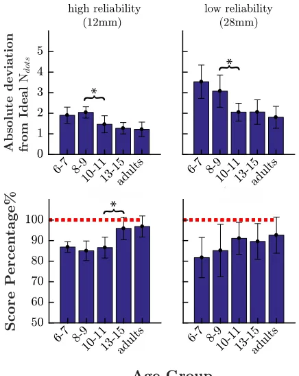
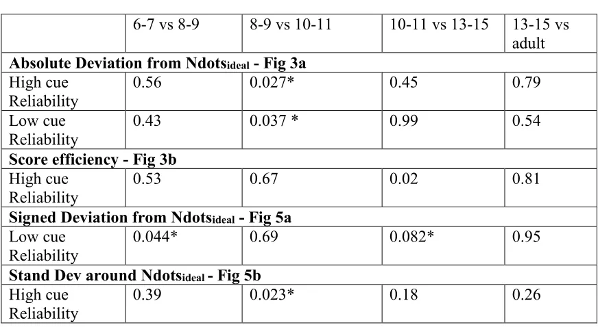
Figure 3A plots group means and 95% CIs for this measure. The ANOVA’s we performed revealed that the deviation from the ideal sampling strategy decreased significantly with age in both cue reliability conditions (high reliability cues:
F(4,69)=4.77, p=0.002; low reliability cues: F(4,71)=5.2, p=0.001). Information sampling
efficiency thus improved with age. However, individual sampling decisions were often suboptimal at all ages: analyses of individual participants using Bonferroni-corrected one-sample t-tests (113 tests, p < 0.00044) revealed significant differences between Ndots sampled and Nideal in 25 out of 27 6-7 year-olds (93%), 22 out of 30 8-9 year-olds
(73%), 23 out of 27 10-11-year-olds (85%), 21 out of 29 teenagers (72%), and 23 out of 29 adults (79%). Thus, although adults were more efficient and closer to their ideal sampling strategy than children, many individuals still exhibited suboptimal sampling strategies.
To test how these age-differences in visual information sampling affected task-performance, we predicted what participants’ score could have been if they had used their own ideal strategy on every trial. The “score percentage” is the percentage of this ideal score that was actually obtained (Figure 3B). Score percentage increased
pattern was observed in the low cue reliability condition, this effect was not
statistically significant (F(4,71)=0.8, p=0.53). This might be because deviating from the
[image:17.595.87.305.184.458.2]ideal strategy in the low cue reliability condition resulted in smaller reductions in hit probability, and hence a lower cost to performance (less steep expected gain curves (red) in bottom vs. top panel of Figs 2 and 4).
Figure 3. A. Mean absolute deviation from the gain-maximizing strategy (mean ± 95%CI). B. score percentage, the percentage of the best score prediction (set to 100%, red dotted line) actually obtained. Stars indicate significant
Younger children’s sampling strategies deviated more from ideal sampling than those of adults and this reduced their score. Sampling strategies became increasingly more efficient with age and started to resemble those of adults from approximately age 10 years onwards (see Figure 3., and Supplementary Table S1). Adolescence --- the period between age 11 years and adulthood --- is often linked to more risky behavior in real life, and it was recently suggested that this may in part be due to a reduced
tendency to seek out information about probabilities (Van den Bos & Hertwig, 2017). In the current experiment deviations between the ideal and sampled Ndots were closest
to those of adults in adolescents. This outcome suggests that the ability to balance costs and benefits to optimize visual information sampling, develops around age 10 years or soon thereafter, and follows an incremental rather than a U-shaped trajectory.
Age differences in Sampling Bias and Variability
To understand why younger children’s sampling choices were inefficient, we investigated in which specific ways (outlined in Fig 2) they deviated from the ideal observer. In Figure 4 we have plotted the individual sampling strategies (mean Ndots)
against the scores obtained for each age group, as well as the age-specific expected gain across Ndots (red “expected gain” curves; thick lines are group averages, thin lines
are individuals) and the ideal strategy (dotted line). Positive values indicate over-sampling and negative values under-over-sampling. The average ideal Ndots and observed
Ndots are displayed for each age group in Table 1. Notably, the data points in all age
Figure 4: Red data points show the numbers of dots sampled per trial plotted against trial scores (means and 95%CI). Scores are shown as proportion of the maximum trial score (20). Red curves indicate the expected gain for each Ndots (thick curves show group averages; thin curves show individuals). Note that these curves indicate the expected score for the scenario in which the corresponding Ndots is sampled on every single trial. The ideal Ndots was computed separately for each individual based on their observed hit rates in the fixed-dot condition; see Methods. Therefore, the gain-maximizing strategy/peak of the gain curves is centered on zero so that deviations from the ideal strategy are comparable across participants. See Table 1 for average group values.
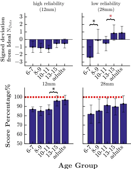
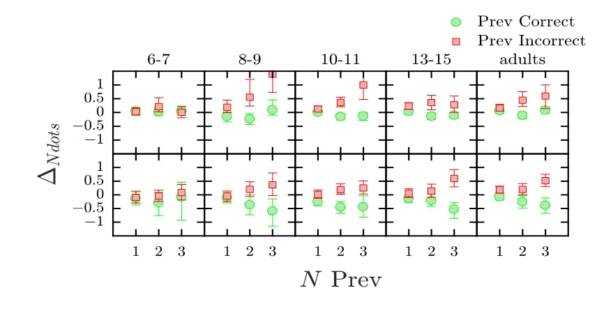
Figure 5. A: Group-mean sampling bias as indexed by the signed deviation from the ideal sampling strategy (mean ± 95%CI). Negative values indicate a tendency to under-sample. Positive values indicate a tendency to over-sample. B: Group-mean sampling consistency as indexed by the Standard Deviation of sampled Ndots. Stars indicate significant differences or trends across consecutive age groups (black: p<0.05, red: p<0.1 see
[image:19.595.89.318.372.666.2]Age Differences in Sampling Bias?
First we tested if reductions in performance efficiency in childhood were due to a systematic tendency to under- or over-sample (sampling bias). Either bias would result in a reduction in expected gain - in the case of under-sampling because observers played for higher points at an overly great chance of missing the target, and in the case of under-sampling because observers improved their hit-rate at an overly great loss of target value (Figure 2, squares and diamonds). To test for age differences in sampling bias, we computed the mean signed deviation from the optimal sampling strategy (sampled Ndots – ideal Ndots; Figure 5A). Within the low reliability condition, there was
a significant shift from under-sampling at the youngest ages to slight over-sampling in adults (F(4,71)=4.55, p=0.003). In the high reliability condition, children of all ages
significantly under-sampled while adults did not show any sampling bias, but the age difference in bias was not significant (F(4,69)=1.11, p=0.36). Together these findings
reveal a developmental shift from under-sampling in the youngest children, towards more extensive and closer-to-ideal sampling in older children and adults.
Age Differences in Trial-to-Trial Sampling Variability?
Next, we tested whether variability in sampling strategy could also have contributed to reductions in performance efficiency in childhood. The ideal observer in this
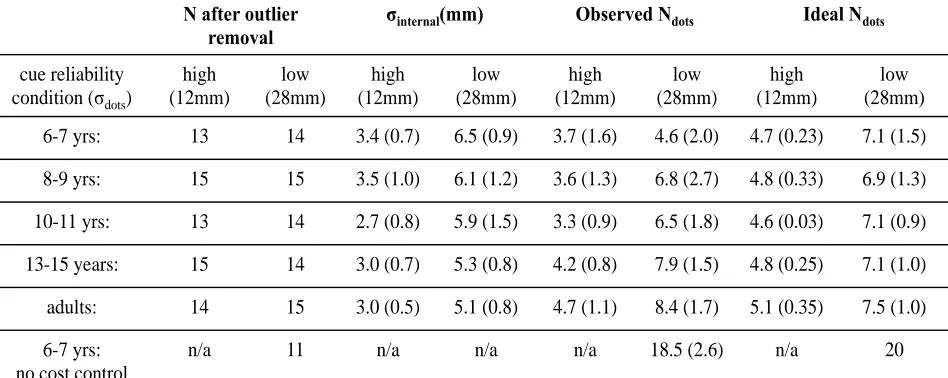
[image:20.595.81.555.69.258.2]experiment should never deviate from the optimal sampling strategy, as any variation comes at some cost to expected gain (Juni et al., 2016). To test for age-differences in sampling consistency, we compared the standard deviation of the Ndots sampled. For Table 1. For each age group and condition, the number of subjects after outlier removal (columns 2-3), σinternal: mean standard deviation of aiming variance around the middle of the dot-cloud (see
Supplementary Materials S1, from the fixed Ndots condition (columns 4-5), sampled Ndots (columns 6-7), and Ideal Ndots (columns 8-9).
N after outlier removal
σinternal(mm) Observed Ndots Ideal Ndots
cue reliability condition (σdots)
high (12mm) low (28mm) high (12mm) low (28mm) high (12mm) low (28mm) high (12mm) low (28mm)
6-7 yrs: 13 14 3.4 (0.7) 6.5 (0.9) 3.7 (1.6) 4.6 (2.0) 4.7 (0.23) 7.1 (1.5)
8-9 yrs: 15 15 3.5 (1.0) 6.1 (1.2) 3.6 (1.3) 6.8 (2.7) 4.8 (0.33) 6.9 (1.3)
10-11 yrs: 13 14 2.7 (0.8) 5.9 (1.5) 3.3 (0.9) 6.5 (1.8) 4.6 (0.03) 7.1 (0.9)
13-15 years: 15 14 3.0 (0.7) 5.3 (0.8) 4.2 (0.8) 7.9 (1.5) 4.8 (0.25) 7.1 (1.0)
adults: 14 15 3.0 (0.5) 5.1 (0.8) 4.7 (1.1) 8.4 (1.7) 5.1 (0.35) 7.5 (1.0)
6-7 yrs: no cost control
cues with high reliability, sampling was significantly more variable at younger ages (F(4,69)=2.81, p=0.03; Figure 5B. But the age-related decrease in sampling variability
was not significant for cues with low reliability (F(4,71)=0.57, p=0.69). Thus, at least for
high reliability cues, greater variability in sampling over the course of the study likely contributed to children’s poorer performance.
Which processes underlie these age-differences in sampling?
The foregoing analyses show that information sampling develops across childhood, with closer-to-ideal sampling strategies resulting in higher target localization scores. This development was paired with a shift from systematic under-sampling of visual information towards sampling the amount that offers a perfect trade-off between information costs and benefits, as well as with less variation in the sampling strategies selected. What processes could give rise to this developmental shift in sampling choices? In the following section we present additional analyses, data, and simulation to test 4 potential explanations:
Do children’s sampling strategies deviate more from the ideal because:
1. It takes the developing system longer to learn the optimal sampling strategy over the course of the task (Age differences in learning)?
2. Younger children assign additional intrinsic cost to sampling, for example due to fatigue or boredom (Age differences in sampling costs)?
3. Children’s stopping rule is more heavily influenced by information that appears to provide information about hit probability but is in fact misleading, such as dot-spread or trial-to-trial fluctuations in performance (Age differences in sensitivity to probability information)?
4. Children are in fact making a correct trade-off between hit probability and target value, but their probability representation is noisy or biased (Age differences in the visual uncertainty estimate)?
1) Age Differences in Learning?
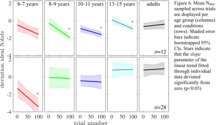
reinforcement learning to identify the ideal strategy. To investigate contributions of such learning, we tested whether participants’ sampling decisions improved over the course of the task and how this differed across age groups (Figure 6).
We fitted linear trends to individual deviations from the ideal Ndots across the
100 experimental trials to quantify shifts towards or away from the ideal sampling strategy. We then compared the slopes across age. For cues with high reliability, there was a significant overall shift towards more under-sampling over the course of the task (slope < 0; t(54)= -3.0687, p=0.0034). This main effect was driven primarily by
children; Adults did not change their sampling strategy significantly (t(13)=-0.82,
p=0.43) while children’s sample sizes decreased over time, although this pattern did not reach statistical significance in the youngest age group (10-11 t(12)= -2.49, p = 0.03; 8-9: t(14) = -2.95, p = 0.01; 6-7 t(12) = -1.53, p = 0.15). There was a marginal age difference in slope (F(3,51)=2.75, p=0.05). In the low cue reliability condition,
sampling strategies did not change substantially with age; slopes did not deviate significantly from zero t(57)= -1.3408, p= 0.19, and did not differ significantly with age
(F(3,54)=1,70, p=0.17). In short, adults immediately chose their sampling strategy from
the start of the task, suggesting they rapidly inferred a close to - though not perfectly - ideal strategy and/or were very fast learners. In contrast, younger participants
[image:22.595.78.513.537.790.2]consistently under sampled, and if anything, moved further away from the ideal strategy over the course of the task, despite receiving constant feedback about their score. Given that there was little evidence for reinforcement learning at any age, a slower learning rate is unlikely to fully explain the age differences in sampling.
Figure 6. Mean Ndots sampled across trials are displayed per age group (columns) and conditions (rows). Shaded error bars indicate bootstrapped 95% CIs. Stars indicate that the slope
2) Age Differences in Sampling Costs?
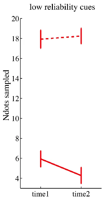
A tendency to gather too little information in younger children could be explained by fatigue or boredom, as such factors may impose additional (implicit) costs on dot-sampling that were not accounted for in the explicit cost function of the ideal observer model. To test this, we performed a control experiment with a new cohort of children from the youngest age group (the age group that most exhibited under-sampling in the first experiment). Eleven 6 to 7-year-olds performed the same low cue-reliability condition from the main experiment (see Methods), the only difference was that the cost of sampling more dots was reduced from 1 to 0 (i.e., target-worth remained at 20 points throughout, irrespective of the number of dots Ndots sampled). Clearly, the
gain-maximizing strategy in this case is to sample all 20 dots on every trial. This requires frequent button pressing and long test durations, which should amplify any effects of fatigue or boredom. Nevertheless, 6 to 7-year-olds sampled substantially more dots than before, and did not deviate from the gain-maximizing strategy by any greater extent than in the main task (18.5 vs. 20 as compared with 4.6 vs 7.2). Moreover, they did not reduce their sampling over the course of the experiment (sampled Ndots start
(1-15)= 17.9 (SD=3.5), sampled Ndotsend(85-100)= 18.2; (SD=2.9); see Supplementary Figure
S3). Thus, it is unlikely that young children’s tendency to under-sample information in the main experiment was due to fatigue, boredom, lack of motivation, or failure to comprehend the task. These results also confirm that even the youngest children had at least some understanding of the ‘probability x value’ structure of the task, since they sensibly sampled more information when there were no explicit sampling costs.
3. Age differences in Sensitivity to Probabilistic Information?
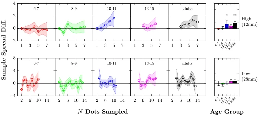
Juni et al. (2016) showed that one reason why adults in their experiment varied their sample sizes from trial to trial was that they adjusted their sampling strategy to the spread of the sampled dots, sampling more when dot positions were far apart. This strategy is suboptimal: when underlying sampling distributions have a fixed standard deviation, hit probability is independent of sample spread, which is something
To test whether this false intuition might explain the more variable and less efficient sampling observed in childhood, we extracted the observed dot configurations for every trial in which participants viewed 3-14 Ndots (data for other conditions were too
sparse). For each dot configuration, sample spread was computed as the Root Mean Square (RMS) distance of the points from the arithmetic mean. The set of RMS values was then divided into two types (RMSstop vs. RMScont.), depending on whether the
observer stopped sampling at this point or continued to sample more dots on that trial. Finally, we computed the mean Sample Spread Difference (SSD) between the two trial types,
SSD = RMScont – RMSstop,
and used bootstrapping to compute 95% confidence intervals. If observers were more likely to keep sampling when dot-cue spread was high, then SSD would be positive. In contrast, if --- as per the ideal observer --- sampling decisions were made
independently of dot-cue spread, then SSD would be ~0. The results of this analysis are shown in Figure 7. First, let us consider the High Reliability (σdots = 12 mm)
condition. Up to the ages of 8 to 9 years sampling choices were independent of dot-cue spread. A tendency to sample more dots when sample variance was greater, especially as Ndots increased present in adults (p<0.01), emerged around age 10-11 yrs. (p<0.05),
although this pattern did not reach statistical significance in adolescents. In the Low Reliability (σdots = 28 mm) condition, there was no effect of sample variance for any
[image:24.595.90.519.63.253.2]age groups.
Thus, in keeping with previous findings (Juni et al. 2016) adults and older children’s stopping rules were (incorrectly) affected by dot sample variance in the high reliability condition, while younger children were affected less or
inconsistently by dot-cue spread. There was no significant effect of dot cue spread on sampling strategy at any age for Low Reliability cues. Developmental changes in visual sampling such as reduced variance in the Ndots sampled with age - are therefore unlikely to be driven by greater sensitivity to dot-spread in younger participants.
We also tested if greater susceptibility to hits and misses on previous trials could explain greater variance in sampling behaviour in the younger age groups, and found this not to be the case (see Supplementary Figure S4). This analysis showed that participants aged 8-9 years and older, all sampled more Ndots following series of misses than after series of hits, but that the youngest children did not adjust their sampling significantly depending on previous trial success. This suggests that adults and older children may use feedback in similar ways to fine-tune their sampling strategy, but that younger children appeared to ignore feedback altogether.
4) Age Differences in the Visual Uncertainty Estimate?
We next explored whether the tendency to under-sample in younger children may in fact be adaptive if you have an imperfect estimate of visual uncertainty. The ideal observer model we used to analyse the data (e.g., Figures 2 and 3), assumes that participants are perfectly aware of how their chances of hitting the target increases with Ndots (i.e., σobs; see Supplementary Figure S1). However, participants may have
had some error or bias in their estimate of response precision, and this may be more extreme in childhood. Could children’s sampling choices in fact be maximising score considering such plausible limitations?
To test this, we first computed the ideal sampling strategy for an observer with a noisy but unbiased estimate of how hit probability changes with dot sample size. Details on how this model was computed are provided in Supplementary Figures S5 and S6. With increasing amounts of error in the hit probability estimate, this noisy ideal observer sampled fewer dots than the ideal observer with a perfect hit probability estimate (see Supplementary Figure S5). Importantly, however, even for large error in the visual uncertainty estimate, the reduction in the ideal Ndots to sample was only
It is also possible that the sampling choices in young children might be explained by a systematic bias in the estimated chance to hit the target. Since we had no a-priori reason to assume that children systematically under- or overestimate the precision of their location estimate, we considered how processing limitations known to characterise development (i.e., limited memory), might give rise to such a bias; one way in which participants might estimate visual uncertainty for a given sample size, is by directly tracking the deviations between each location guess and the target location. An observer considering only a limited number of previous trials to compute the deviation between location guesses and target due to limited memory for a given Ndots, will overestimate the true chance of hitting the target (see Supplementary Figure S6 for simulations). However, when we simulated an observer with the maximal bias that this strategy could result in, combined with the highest possible amount of uncertainty around this biased estimate of hit probability that we could model, the ideal sampling strategy was still slightly higher than the Ndots observed in young children (Ndots at age
6-7 = 4.6, ideal Ndots for the most noisy and biased ideal observer = 5.6 dots), although
it started approaching child behaviour. So, a similar process could contribute to the tendency to under-sample in childhood, but is unlikely to fully explain it.
Discussion
The youngest children markedly deviated from the gain-maximizing strategy (Figure 3A), and scored less well on the task (Figure 3B). With age, sampling choices gradually shifted towards the ideal strategy so that by 10-11 years, children’s sampling resembled the near optimal performance of adults. Younger children’s sampling choices were less efficient in that they (a) showed a systematic bias towards under-sampling, and (b) showed more variation in the numbers of dots sampled (Figure 4 and 5). While this pattern was observed for both cue reliabilities, not all age differences reached statistical significance in both cue conditions. This is likely because the conditions differed in their sensitivity to these different aspects of sampling efficiency. For example, given the strongly peaked gain-landscape for high reliability cues, a suboptimal strategy was penalized more heavily and caused greater loss of points. Instead, for low reliability cues, there was more room for under-sampling because the ideal strategy was not compressed towards the lower end of the scale.
Taken together, the data suggested a gradual age-related improvement in visual sampling, with adult-like performance reached around age 10-11 years or soon
thereafter. Below we discuss the processes that might give rise to this development, based on our further analyses and control experiments.
More variable sampling in childhood
For each experimental condition there was only one optimal strategy and the
participant should choose the same (optimal) number of samples on every trial. The ideal observer would always take the same number of samples in each trial of an experimental condition (Juni et al., 2016). In contrast, our human observers were prone to vary the number of cues sampled across trials, and this tendency was particularly pronounced in younger children.
Interestingly, however, even though children in the current study were more variable in their sampling strategies, we found no evidence of learning across trials. If anything, younger participants moved away from the ideal strategy over the course of the session (Figure 6). We therefore considered another factor that might contribute to children’s more variable sampling; an over-sensitivity to task-irrelevant information, such as trial-by-trial variations in the spread of the dot cues, and/or the outcomes of previous trials. Whilst an ideal observer with perfect understanding of the hit
probabilities in the current task should ignore these cues, a more realistic observer with imperfect knowledge about dot cue reliability and their own averaging skills might use these cues, to inform their sampling decisions.
Adults and older children did sample more information when the spread of the existing dot-cues on the screen was high (in line with findings by Juni et al), and when they experienced a run of misses in the immediately preceding trials. However, there was no evidence for sensitivity to these cues in the youngest children. While children varied the number of samples taken from trial to trial, in line with a preference for novelty and exploration we could not identify factors indicative of learning that lead them to sample more or less. Moreover, children appeared to be relatively insensitive to information about success probability and visual uncertainty. Instead, as discussed below, more variable sampling in childhood in part reflected a gradual shift towards a strategy with greater potential rewards but lower expected gain in the long run.
Under-sampling
Under-sampling on this task can be described as risk-seeking because it involves playing for higher stakes at a greater chance of losing, thus favouring a greater range of possible outcomes (e.g., 16 or 0 points) over sampling strategies with a smaller outcome range (e.g., 12 or 0 points) but a higher expected score. This is a standard definition of risky choice behaviour (Defoe et al., 2015).
We considered several factors that could potentially account for children’s tendency to under-sample. Firstly, we explored whether children’s sampling decisions might be explained by intrinsic cost factors not captured in the ideal observer model in Figure 2, such as fatigue or boredom. We did this by running a control experiment in which sampling more dots incurred no point-loss. 6- to 7-year-olds in this situation, sampled substantially more than the children in the main experiment. Crucially, despite making more button-presses and enduring longer trials, these children did not reduce their sampling over the course of the control task. This outcome implies that children’s substantial under-sampling in the main experiment is unlikely to be due to fatigue, lack of motivation, or some other implicit sampling cost. Interestingly, this comparison of main and control tasks revealed a sensitivity to both value and
probability information even at the youngest ages of 6-7 years: children sampled much less when sampling incurred a point loss (~4.6 dots, main task), than when sampling improved the probability of success without any loss (~18.5 dots, control task). Still, while 6 to 7-year-old children were sensitive to both value and probability, their sampling decisions were less efficient than those of older children and adults.
We next tested whether the trade-off children made in the main task might in fact be considered optimal if we assumed noise and/or bias in the estimate of visual uncertainty and target hit probabilities. To explore this possibility, we first simulated the effects of adding Gaussian noise to an observer’s internal estimate of their own visual uncertainty. The largest amount of error that we were able to model (assuming equal likelihood of under- or over-estimation) only predicted a small reduction in sampling, suggesting that this factor alone is unlikely to explain child performance.
small number of trials (i.e., given limited memory) total variance will be underestimated. We showed that the most extreme underestimation of visual uncertainty from this process, combined with the largest error that we could model around this biased estimate, came closer to but still did not fully capture the extent of under-sampling in the youngest age group (Ndots = 5.6 in simulation, while the
youngest children sampled Ndots = 4.6 on average).
Of course, any data can be fitted given sufficient assumptions about underlying parameters. However, the fact that these relatively parsimonious changes to our ideal observer model unable to explain the level of under-sampling exhibited by young children suggests that their inefficiency is unlikely only due to poor insight in their own visuomotor abilities, although it is possible that such limitations play some role (see below).
Developmental mechanisms of decision-making during sampling
Adults and older children select the gain-maximizing strategy from the start of
the visual sampling task, suggesting that they can rapidly learn to estimate and
compute with probabilistic visuomotor information. Here we show that this ability
takes until ~age 10-11 years to develop. While more research is needed to understand
the mechanisms that drive this developmental shift towards increasingly optimal visual sampling choices, we can formulate some tentative hypotheses based on current data. Our analyses indicate that younger children were less sensitive to misleading
information that adults and older children. They did not take more samples after a series of trials ending in failure or when the cues in a sample were more spread out. In addition, children’s performance did not move toward the ideal strategy even after extensive experience - the trend was in the opposite direction. In additions, simulations revealed that under-sampling at younger ages is not well-captured by a
decision-process that optimally compensates for a poor representation of visual uncertainty due to limitations of memory, or to understanding of how this cue affects hit probability.
putting less weight on this factor, or because the mechanisms needed to scale cost by probability are themselves still developing.
This interpretation is in line with at least two developmental theories of decision-making. The first stems from the perceptual decision-making literature and posits that children have difficulty accounting for the precision of perceptual estimates when combining different types of information, because senses are still calibrating. If it is unclear how a sensory estimate maps onto world, it is best ignored (Gori et al., 2008). It is possible that similar process might constrain younger children’s ability to scale the potential value of the target correctly by their estimate of uncertainty about the targets position.
The result is also in line with a second, conceptually related set of theories in cognitive decision-making: dual systems or “cognitive imbalance” theories. These theories posit that reduced risk-taking in childhood and adolescence reflects high sensitivity to reward, combined with a reduced control mechanism that suppresses potentially hazardous responses – i.e., responses where the likelihood of failure is high (Boyer, 2006; Shulman et al., 2016; Steinberg, 2008). While these dual system models typically presume that risk-taking actually increases in adolescence because hormonal fluctuations increase imbalance between neural motivation and control processes, in the present study the performance improved monotonically throughout childhood.
This result is in line with a recent meta-analysis of decision-making across childhood and adolescence, concluding that most evidence suggests that playing for higher-but-riskier stakes decreases linearly (Defoe, Dubas, Figner, & van Aken, 2015). However, the results reported here contrast with a recent empirical study by Van den Bos & Hertwig (2017), who reported a U-shaped developmental change in
performance on a cognitive sampling task, across childhood, adolescence, and
adulthood. Specifically, 8 year-olds and adults collected similar numbers of samples to learn the payoff structure of two lotteries before making a final choice for points, whilst teenagers sampled significantly less (Van den Bos & Hertwig, 2017).
These discrepant results likely reflect differences between the two tasks and the tested age range. In the current study, inefficient sampling was most
benefits are experimentally defined, and can be inferred directly from the dot-distribution and point system. Consequently, the types of sampling trade-offs in the current task likely rely less on intrinsic cost factors that may distinguish teenage sampling preferences, such as motivation to seek information when the benefit is unclear (i.e., when rare events have unknown likelihoods and consequences; Van den Bos & Hertwig, 2017). The discrepancy across these two studies indicates that the development of sampling behavior in childhood and adolescence might be driven by different factors, highlighting the importance of understanding which component-processes drive suboptimal behavior across different stages of development and different task-domains (Nardini & Dekker, 2018).
What factors may explain difference in performance across visuomotor
sampling and cognitive sampling tasks more broadly? Researchers have investigated
many different sampling tasks (see Introduction) that potentially differ in the
"cognitive operations" needed to carry them out. For example, one key step in our task
is computation of the centroid of a display of points, a "visual routine" in Ullman's
terms (Ullman, 1984), and an example of a cognitive operation that is a component of
visual cognition. Is the efficient performance we observe in older children,
adolescents, and adults, due to the fact that they can tap into powerful visual routines?
Indeed we found that younger children (who have difficulty with centroid
computation; Jones & Dekker, 2017) also did less well.
Could the efficient performance observed be due to some other aspect of our
task not shared with other sampling tasks where human performance is less efficient?
We simply do not know what these key different processes are. Understanding how
different cognitive operations support efficient and less efficient aspects of human
performance is an important goal of research (Trabasso et al., 1978) but much remains
to be done (Nardini & Dekker, 2018; Rahnev & Denison, 2018). Some task differences
may be inconsequential while others may be of great importance. The evident way to
work out which processes explain performance across different sampling tasks is to
design tasks that are identical except in one respect. Wu, Delgado, & Maloney (2009),
for example, compared human performance in decision under risk and in a
mathematically equivalent visuo-motor task. Only the source of uncertainty differed in
the two tasks. At first glance, the planning of movements would seems to have little in
common with decision under risk but the two proved to be remarkably similar
Implications for perceptual development and decisions in the real world
The ability to trade-off the benefits and costs of gathering new data captured by our
visual sampling task is central to success in a wide range of tasks in real life. Whether
navigating traffic, playing sports, or deciding how long to study for an exam, both
looking too little will reduce expected utility – and hence overall success – of our
actions in the long run. Even the youngest children tested displayed a basic
understanding this nuance, since they did not simply maximise hit-rate or potential
score. However, they failed to find the optimal trade-off between the costs and benefits
of sampling that secures the best performance, sampling substantially less information
than they should have to maximise performance. This suggests that previously
observed delays in development of efficient decision-making in childhood also extend
to elementary information-gathering decisions during visuomotor tasks. A tendency to
sample too little information to maximise performance in real-life tasks such as
crossing a busy road, could have serious consequences for child safety. Therefore,
having established that children make inefficient visual sampling choices in our
well-controlled reaching task, future studies should investigate how this extends to real-life
decision-making, using tasks in which sampling costs are defined implicitly and that
involve more complex body movements and visual scenes.
The sampling inefficiencies documented here, in particular the under-sampling and increased variability observed in younger children, introduce novel factors that may contribute to apparent immaturities in perceptual and motor function in
childhood. This has important implications for interpretation of future developmental findings. Consider, for example, developmental studies on coherent form or motion perception in noise. In a typical task (e.g. (Hadad, Maurer, & Lewis, 2011),
participants need to report the average direction of moving dots (e.g. up vs. down), a process that requires averaging many samples across space and time. When stimuli are not limited in duration (e.g. in Gunn et al., 2002; Hadad et al., 2011), participants decide how long to spend collecting information (e.g. averaging motion directions) before responding. Our results suggest that the late development of perceptual abilities on such tasks – as well as other perceptual tasks in which viewing time may be
controlled by participants - may be due in part to inefficient sampling strategies, rather than – as is more commonly supposed – some inherent inability to extract the
More broadly, we propose that insufficient information sampling is an important component of sub-optimality in childhood perception, action and decision-making, with implications for real-world decision-making under risk and uncertainty. Understanding these implications, and their underlying causes is important because this may generate helpful tools for increasing child safety and wellbeing during tasks that require children to stop looking and start acting in everyday tasks in traffic or sports.
Acknowledgments
Context of the research
We present the novel finding that fundamental visual sampling skills show a prolonged developmental trajectory during childhood, with adult-like proficiency reached only in adolescence. This suggests that age-related improvements on tasks in which viewing time is controlled by the observer, may in part be due to inefficient sampling
strategies, rather than – as more commonly supposed – some inherent inability to extract the necessary perceptual information. This work should therefore inspire future research to test how inefficient trade-offs to ‘look versus respond’ contribute to child performance in in everyday tasks such as road crossing or ball interception, or self-paced visual discrimination.
By testing data-driven hypotheses within the model-based framework of our task, we show that poor performance in early childhood may be due to a suboptimal decision-rule, in which the benefits of information gathering are underweighted or ignored. This fits in with suboptimal cue integration and “reward/inhibition” imbalance models of development, and might be because young children are still forming estimates of how their skills affect performance in new task contexts (i.e., the ability to quickly resolve a new gain-landscape), or because the mechanisms that scale task outcome by probability are still developing. Next studies will be directed at disentangling the contributions of these potential mechanisms.
Our findings also speak to the debate around child versus adolescent decision-making, because unlike in ‘free sampling’ (Van den Bos & Hertwig, 2017), adolescent performance was adult-like on our task, highlighting that different factors may shape poor sampling choices at different ages and in different tasks.
References
Battaglia, P. W., & Schrater, P. R. (2007). Humans trade off viewing time and
movement duration to improve visuomotor accuracy in a fast reaching task.
The Journal of Neuroscience, 27(26), 6984–6994.
Bearden, J. N., Rapoport, A., & Murphy, R. O. (2006). Sequential Observation and
Selection with Rank-Dependent Payoffs: An Experimental Study. Management
Bos, W. van den, & Hertwig, R. (2017). Adolescents display distinctive tolerance to
ambiguity and to uncertainty during risky decision making. Scientific Reports,
7, 40962. https://doi.org/10.1038/srep40962
Boyer, T. W. (2006). The development of risk-taking: A multi-perspective review.
Developmental Review, 26(3), 291–345.
Busemeyer, J. R., & Rapoport, A. (1988). Psychological models of deferred decision
making. Journal of Mathematical Psychology, 32(2), 91–134.
https://doi.org/10.1016/0022-2496(88)90042-9
Cumming, G., & Finch, S. (2005). Inference by eye: confidence intervals and how to
read pictures of data. American Psychologist, 60(2), 170.
Dean, M., Wu, S.-W., & Maloney, L. T. (2007). Trading off speed and accuracy in
rapid, goal-directed movements. Journal of Vision, 7(5), 10.1-12.
https://doi.org/10.1167/7.5.10
Defoe, I. N., Dubas, J. S., Figner, B., & van Aken, M. A. G. (2015). A meta-analysis
on age differences in risky decision making: adolescents versus children and
adults. Psychological Bulletin, 141(1), 48–84.
https://doi.org/10.1037/a0038088
Dudey, T., & Todd, P. M. (2001). Making Good Decisions with Minimal Information:
Simultaneous and Sequential Choice. Journal of Bioeconomics, 3(2–3), 195–
215. https://doi.org/10.1023/A:1020542800376
Ernst, M. O. (2012). Optimal multisensory integration: Assumptions and limits. The
New Handbook of Multisensory Processes. Retrieved from
http://pub.uni-bielefeld.de/publication/2466499
Ernst, M. O., & Banks, M. S. (2002). Humans integrate visual and haptic information
in a statistically optimal fashion. Nature, 415(6870), 429–433.
Evans, L., & Buehner, M. J. (2011). Small samples do not cause greater accuracy--but
clear data may cause small samples: comment on Fiedler and Kareev (2006).
Journal of Experimental Psychology. Learning, Memory, and Cognition, 37(3),
792–799. https://doi.org/10.1037/a0022526
Faisal, A. A., & Wolpert, D. M. (2009). Near optimal combination of sensory and
motor uncertainty in time during a naturalistic perception-action task. Journal
of Neurophysiology, 101(4), 1901–1912.
Feller, W. (1968). An introduction to probability theory and its applications: volume I
(Vol. 3). John Wiley & Sons New York. Retrieved from
http://ca.wiley.com/cda/product/0,,0471257087,00.html
Ferguson, T. S. (1989). Who Solved the Secretary Problem? Statistical Science, 4(3),
282–289. https://doi.org/10.1214/ss/1177012493
Fiedler, K., & Kareev, Y. (2011). Clarifying the advantage of small samples: as it
relates to statistical Wisdom and Cahan’s (2010) normative intuitions. Journal
of Experimental Psychology. Learning, Memory, and Cognition, 37(4), 1039–
1043. https://doi.org/10.1037/a0023259
Gori, M., Del Viva, M., Sandini, G., & Burr, D. C. (2008). Young children do not
integrate visual and haptic form information. Current Biology, 18(9), 694–698.
Gunn, A., Cory, E., Atkinson, J., Braddick, O., Wattam-Bell, J., Guzzetta, A., & Cioni,
G. (2002). Dorsal and ventral stream sensitivity in normal development and
hemiplegia. Neuroreport, 13(6), 843–847.
Gureckis, T. M., & Love, B. C. (2009). Short-term gains, long-term pains: How cues
about state aid learning in dynamic environments. Cognition, 113(3), 293–313.
Hadad, B.-S., Maurer, D., & Lewis, T. L. (2011). Long trajectory for the development
of sensitivity to global and biological motion. Developmental Science, 14(6),
1330–1339.
Hau, R., Pleskac, T. J., Kiefer, J., & Hertwig, R. (2008). The description–experience
gap in risky choice: the role of sample size and experienced probabilities.
Journal of Behavioral Decision Making, 21(5), 493–518.
https://doi.org/10.1002/bdm.598
Hertwig, R., Barron, G., Weber, E. U., & Erev, I. (2004). Decisions from Experience
and the Effect of Rare Events in Risky Choice. Psychological Science, 15(8),
534–539. https://doi.org/10.1111/j.0956-7976.2004.00715.x
Hertwig, R., & Pleskac, T. J. (2010). Decisions from experience: Why small samples?
Cognition, 115(2), 225–237.
Jones, P. R. (2018). The development of perceptual averaging: Efficiency metrics in
children and adults using a multiple-observation sound-localization task. The
Journal of the Acoustical Society of America, 144(1), 228–241.
https://doi.org/10.1121/1.5043394
Jones, P. R., & Dekker, T. M. (n.d.). The development of perceptual averaging:
learning what to do, not just how to do it. Developmental Science, 21(3),
e12584. https://doi.org/10.1111/desc.12584
Juni, M. Z., Gureckis, T. M., & Maloney, L. T. (2016). Information sampling behavior
with explicit sampling costs. Decision, 3(3), 147–168.
https://doi.org/10.1037/dec0000045
Kahan, J. P., Rapoport, A., & Jones, L. V. (1967). Decision making in a sequential
search task. Perception & Psychophysics, 2(8), 374–376.
Kleiner, M., Brainard, D., Pelli, D., Ingling, A., Murray, R., Broussard, C., & others.
(2007). What’s new in Psychtoolbox-3. Perception, 36(14), 1.
Levin, I. P., Hart, S. S., Weller, J. A., & Harshman, L. A. (2007). Stability of choices
in a risky decision-making task: a 3-year longitudinal study with children and
adults. Journal of Behavioral Decision Making, 20(3), 241–252.
https://doi.org/10.1002/bdm.552
Mood, A. M., Graybill, F. A., & Boes, D. (1974). Introduction to the theory of
statistics, McGraw-Hill. DaCosta, CJ and Baenziger, JE et Al (2003). A Rapid
Method for Assessing Lipid: Protein and Detergent: Protein Ratios in
Membrane–Protein Crystallization, 59, 77–83.
Nardini, M., Bedford, R., & Mareschal, D. (2010). Fusion of visual cues is not
mandatory in children. Proceedings of the National Academy of Sciences,
107(39), 17041.
Nardini, Marko, & Dekker, T. M. (2018). Observer models of perceptual development.
Behavioral and Brain Sciences, 41.
https://doi.org/10.1017/S0140525X1800136X
Nardini, Marko, Jones, P., Bedford, R., & Braddick, O. (2008). Development of cue
integration in human navigation. Current Biology, 18(9), 689–693.
Rahnev, D., & Denison, R. N. (2018). Suboptimality in Perceptual Decision Making.
The Behavioral and Brain Sciences, 1–107.
https://doi.org/10.1017/S0140525X18000936
Rakow, T., Demes, K. A., & Newell, B. R. (2008). Biased samples not mode of
presentation: Re-examining the apparent underweighting of rare events in
experience-based choice. Organizational Behavior and Human Decision