Optimization of Long-Run Average-Flow Cost in Networks With Time-Varying Unknown Demand

Time-Varying Unknown Demand

.

White Rose Research Online URL for this paper:

http://eprints.whiterose.ac.uk/89734/

Version: Accepted Version

Article:

Bauso, D., Blanchini, F. and Pesenti, R. (2009) Optimization of Long-Run Average-Flow

Cost in Networks With Time-Varying Unknown Demand. IEEE Transactions on Automatic

Control, 55 (1). 20 -31. ISSN 0018-9286

https://doi.org/10.1109/TAC.2009.2034204

[email protected] https://eprints.whiterose.ac.uk/ Reuse

Unless indicated otherwise, fulltext items are protected by copyright with all rights reserved. The copyright exception in section 29 of the Copyright, Designs and Patents Act 1988 allows the making of a single copy solely for the purpose of non-commercial research or private study within the limits of fair dealing. The publisher or other rights-holder may allow further reproduction and re-use of this version - refer to the White Rose Research Online record for this item. Where records identify the publisher as the copyright holder, users can verify any specific terms of use on the publisher’s website.

Takedown

If you consider content in White Rose Research Online to be in breach of UK law, please notify us by

Optimization of Long-run Average-Flow Cost in

Networks with time-varying unknown demand

D. Bauso, F. Blanchini and R. Pesenti

Abstract— We consider continuous-time robust network flows

with capacity constraints and unknown but bounded time-varying demand. We consider the problem of designing a control strategy, to regulate the flow on-line with no knowledge off– line of the demand realization. We address both the case of systems without and with buffers. The main novelty in this work is that we consider a convex cost which is a function of the long-run average–flows and average–demand. We distinguish a worst-case scenario where the demand is the worst-one from a deterministic scenario where the demand has a neutral behavior. The resulting strategies are called min-max or deterministically optimal respectively. The main contribution are constructive methods to design either min-max or deterministically optimal strategies. We prove that while the min-max optimal strategy is memoryless, i.e., it is a piece-wise affine function of the current demand, deterministically optimal strategy must keep memory of the average flow up to the current time.

I. INTRODUCTION

We frame this work within the several recent attempts to apply the tools of robust optimization to network flows [1], [2], [10], [11], [18], [23], [24].

Network flows describe flows of materials between different production/distribution sites (see, e.g., [25]). The problem is to design a strategy that returns the controlled flow as a function of the uncertain and time-varying demand.

Robust optimization is a relatively recent technique that de-scribes uncertainty via sets and optimizes the worst-case cost over those sets (see, e.g., the introduction to the special issue [6]). Generally speaking, robust optimization aims at achieving the best cost under the worst uncertainty conditions. Some of the existing works (in particular [2], [11]) are centered around the idea of “adjusting” some of the variables to the outcome of the uncertainty. In other words some variables are decided before the uncertainty realization while the rest are decided after the uncertainty realization. Such a problem formulation is known under different names such as “Adjustable Robust Counterpart” (ARC) problem, “Two-stage Robust optimization with recourse”. In many cases the adjustable variables are ex-pressed affinely on the uncertainty and the problem is renamed Affinely Adjustable Robust Counterpart (AARC) problem. ARC and AARC formulations are currently a hot topic in the mathematical programming and operations research field. There are interesting connections between this paper and the notions of “adjustable variables” in ARC, AARC. For instance,

Dip. di Ingegneria Informatica, Universit`a di Palermo, Viale delle Scienze, I-90128 Palermo, Italy, [email protected]

Dip. di Matematica e Informatica, Universit`a di Udine, Via delle Scienze 206, 33100 Udine, [email protected] – Corresponding Author

Dip. di Matematica Applicata, Universit`a Ca’ Foscari Ca’ Dolfin - Dorso-duro 3825/E - 30123 Venezia, Italy, [email protected]

the flow plays the role of the adjustable variables in the ARC set up and in most cases the strategy is affine in the uncertainty as in AARC problems.

In this paper, we address both the cases of networks without buffers and networks with buffers. If no buffer are present, incoming and outcoming flows at each site are equal since there is no stored inventory. In this case we also say that flows balance the demand. In the case of networks with buffers, inventory accumulate at the production sites as result of the discrepancy between incoming and outcoming flows. According to existing work in the control literature [13], [14], [15], [16], [17], [21], buffers’ dynamics is described by linear continuous-time differential equations.

In our model there are two types of flows the controlled one and the uncontrolled one. For brevity, these we will use the terms “flow” to mean the controlled one and “demand” to mean uncontrolled one, although there are many realistic situations in which an uncontrolled flow is not a demand. We assume that both flow and demand lie in pre-defined polytopes. The basic problem is that of designing off-line a strategy, namely a control law for the flow. The flow will be computed on-line, on the basis of the measured buffer levels (if any) and demand by means of the provided strategy. The actual realization of the demand is not available in the design stage. In networks with buffers, we impose the buffer level to reach a prescribed level in finite time up to an assigned toleranceε>0. The associated strategy is calledε-stabilizing (this problem is also know as “target set reachability” see [8], [9]).

We consider causal strategies of different types. Precisely we consider the case in which the flow is i) a function of the current demand (memoryless strategy), ii) a function of the current and past demand (strategy with memory), iii) a function of the buffer levels and past demand (feedback strategy), and iv) a function of the buffer levels (memoryless feedback strategy).

We deal with both a worst-case (call it also min-max) and a deterministic scenario. In the min-max (pessimistic) approach the realization maximizes the value of the given cost. In the deterministic scenario, the demand is just any arbitrary realization. Depending on the approach, the resulting strategy is said min-max or deterministically optimal respectively.

Motivations of this choice may derive from technical rea-sons, contracts or agreements. For instance, technical reasons or contracts may establish the long-run exploitation level of the machineries. So, over or under-utilization of machineries can be tolerated only temporarily and not persistently. In a different situation, long-term agreements may establish priv-ileged sources for each destination. So, a mismatch between privileged sources and destinations is acceptable only in crit-ical and rare cases.

As a basic result we provide a constructive method to design a piecewise affine strategy which is min-max optimal. The method is based on the fact that the min-max problem arising when flow and demand are time-varying is equivalent to the min-max problem in which flow and demand are constant vectors (one-shot decisions) and not functions of time.

The obtained strategy is memoryless and such a result allows us to conclude that memory is not required when min-max optimality is considered. We initially derive these results for networks without buffers, and then extend them to networks with buffers.

In the second part of the work, we show that the provided min-max optimal strategy is not deterministically optimal, that is, it does not return the minimal cost for any given realization of the demand. Actually we show that static strategies are not deterministically optimal at all (even for networks without buffers). The second main contribution of the paper is to show that, under some smoothness assumptions on the cost functional, an easily implementable deterministically optimal strategy can be derived. Such a strategy is achieved by keeping memory of the average flow (from the initial to the current time) and by choosing, among the admissible inputs, the instantaneous minimizer of the Lyapunov derivative of the cost of the partial average (i.e. from the beginning to the current time).

The structure of the paper is as follows. In Section II, we describe the problem for a network without buffers. In Section III, we determine a min-max optimal strategy. In Section IV, we extend the study to networks with buffers. In Section V, we design a deterministically optimal strategy under proper assumptions on the cost.

II. PROBLEMDESCRIPTION

Consider a network where at each time the flow balances the demand. Both the flow and the demand are bounded in assigned polytopes. A simple description of such a system is

Bu(t) = w(t), ∀t, (1)

u(t) ∈ U_{, ∀t, (2)}

w(t) ∈ W_{, ∀t, (3)}

where B is the full-row rank matrix representing the network topology, u(t)is the(controlled)flow and w(t)is the demand

(uncontrolled flow). and U _⊂IRm _{andW ⊂IR}n _{are assigned}

polytopes for u and w respectively. To let system (1)-(3) be feasible, that is to admit at least a flow u(t)for any realization of w(t), we must assume that (see [5] for details) the following condition holds

W _⊂BU_.

Given a piecewise-continuous function f : IR+ →IRn we denote by

¯

fT=AvT[f]=.

1 T

Z T

0

f(t)dt

and

¯

f =Av[f]=. lim

T→∞ AvT[f]

the finite-horizon and infinite-horizon average values. The simpler notation ¯f will be often preferred where the meaning is clear from the context. In a similar way, given a sequence

f :N _→IRn_{, we denote by ¯f =lim}

k→∞_T1∑Tk=0 f(k).In the

following, we assume that the average is defined for any function we consider. We generically denote byΦ a strategy of the form

u=Φ(·,w(t)), (4)

where the missing argument(·)represents any set of auxiliary variables. For instance we admit strategies of the form

u(t) = Φ(ξ(t),w(t),t), ˙

ξ(t) = Φ_ξ(ξ(t),u(t),w(t),t), (5)

whereξ is the controller state vector. We do not assume any special requirement for the domain of ξ which can be any functional space and Φ_ξ can be any operator. The following assumption clarifies the information available to the network manager.

Assumption 1:

• The value w(t)is available on–line at time t without delay.

• The realization w is not known in advance so the strategy can rely on the memory of the past values w(τ), τ≤t, but there is no forecast about the future.

We will have a special attention for the simple case of static strategies according to the next definition.

Definition 1: The strategy Φ is called memoryless if it is a function of the current demand only, u(t) =Φ(·,w(t))≡

Φ(w(t)). Otherwise, the strategy Φ(·,w(t)) is called with memory.

Let Ψ(u,w) be a real-valued function representing a cost. In this paper we consider different concepts of optimality as specified next. Henceforth, we use the min-max notation (rather than inf-sup) as we will prove that the problems of interests always admit a minimum and a maximum.

Definition 2: A strategy Φ is min-max optimal (or worst-case optimal) if it is a solution of the problem

min_Φmax_w(·) Ψ(Av[u],Av[w])

s.t. u(t) =Φ(·,w(t))∈U_{, ∀t,}

Bu(t) =w(t), ∀t, w(t)∈W_{, ∀t.}

(6)

Definition 3: A strategy Φ is deterministically optimal if, for any realization of w(·), it is a solution of the problem

minΦ Ψ(Av[u],Av[w])

s.t. u(t) =Φ(·,w(t))∈U_{, ∀t,}

Bu(t) =w(t), ∀t, w(t)∈W_{, ∀}t.

(7)

Given the scalar valuesαk, for k=1,2, . . . ,K we write

c.c.αk, to mean that αk≥0

K

∑

k=1

αk=1

so that, given any set of vectors w(k), we write any convex combination as

w= K

∑

k=1

αkw(k), c.c.αk.

Consider the following assumption for Ψ.

Assumption 2: Function Ψ is convex1 namely for any set

(u(k),w(k))inU _×W _{and c.c.}αk

Ψ³

∑

αku(k),

∑

αkw(k)´≤

∑

αkΨ³u(k),w(k)´. Under convexity assumption we consider the following two problems.

Problem 1: Robust Problem Determine if it exists a static

min-max optimal strategy.

Problem 2: Deterministic Problem Determine if it exists

a deterministically optimal strategy.

As we will see both problems are solvable, but the strategy solution of the Deterministic Problem cannot be static.

In the current formulation, the system has no buffers, so no backlog or surplus is admitted. In Sections IV and V, we generalize the results to networks with buffers.

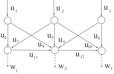
A. A motivating example

Example 1: Consider a resource distribution network whose graph is represented in Fig. 1, with unknown but bounded demand w−_i ≤wi≤wi+, i=1,2,3 and bounded flow 0≤ui≤

u+_i , i=1, . . . ,12. Constraints (1) establish a relation between

u

5

u

₄

u

6

u

₁

u

₂

u

3

w

w

₂

w

₃

1

u

7

u

9

u

10 8

u

[image:4.595.74.275.531.661.2]

u

₁₁

u

₁₂

Fig. 1. The network for the example

demand and flow. In this example, B is the 6×12 (i.e. n=6 and m=12) incidence matrix of the network with n=6 nodes and m=12 (solid) arcs.

It is obvious that a necessary condition for the existence of a balancing flow for any admissible demand is that the maximum incoming flow umax=u+1+u+2+u+3 is greater than or equal to the maximum demand wmax=w+1 +w+2+w+3. Assume that the network manager assigns the privileged source ui to each

demand wi, i=1,2,3, that is, he wishes that each demand

1_{the considered concept is often referred to as “joint convexity”; note that}

we are not requiring just thatΨis convex in both arguments separately

wi is supplied in the long run by the corresponding flows ui.

Now, take for instance, u+₃ =6 and w+₃ =7.2

If for a period w3(t)exceeds the value 6, then u2is forced to supply an extra resource. When this occurs, we can say, roughly speaking, that u2 is over exploited and u3 is under exploited. So, in general, a peak of demand wi might require

the exploitation of flows not directly associated to that demand. The underlying idea is to find a mechanism to balance the exploitation of u2and u3by charging u3(t)more than strictly necessary when w3(t)is low. This goal can be seen as a long-run optimization problem with cost

Ψ(u¯,w¯) =

3

∑

i=1

(w¯i−u¯i)2+ρku¯k2. (8)

The additional term is motivated by the fact that we might be also interested in avoiding high flows in the other arcs, although our theory works withρ=0 as well.

III. MIN-MAX OPTIMALITY

In this section we consider three versions of the robust problem . The first one is formulated without restrictions on the type of strategy which can have a Memory (hence the subscript M).

ΨM = minΦmaxw(·) Ψ(Av[u],Av[w]) s.t. u(t) =Φ(·,w(t))∈U_{, ∀}t,

Bu(t) =w(t), ∀t, w(t)∈W_{, ∀t.}

(9)

In the second version only static strategies are admitted (i.e. Memoryless, hence the subscript ML).

ΨML = minΦmaxw(·) Ψ(Av[u],Av[w]) s.t. u(t) =Φ(w(t))∈U_{, ∀t,}

Bu(t) =w(t), ∀t, w(t)∈W_{, ∀t.}

(10)

The third is a pure static one in which w and u are constant

ΨS = minΦmaxw∈W Ψ(u,w)

s.t. u=Φ(w)∈U_,

Bu=w.

(11)

The main result of this section is to prove that the problems of interests always admit a minimum and a maximum, and that

ΨM=ΨML=ΨS. The static version of the problem will enable

us to determine a min-max optimal strategy. It is intuitive that the worst-case w for the static strategy is assumed on the vertices. What we will show that this is true also for the time-varying problem, precisely that the worst-case w(t) assumes its values on the vertices.

A. Solution to the static version of Problem 1

Let us denote by vert{W_{} the set of vertices of} W _and

by K _{={1,2, . . . ,K} the set of indices of the vertices. The}

static version of Problem 1 can be easily solved as follows.

2_{Franco: e’ un errore parlare di power perche nel caso elettrico non e’}

For each w(k)_{∈vert{W}, solve the following static convex} optimization problems

u(k) = arg minu Ψ(u,w(k))

s.t. u=Φ(w(k))∈U_,

Bu=w(k).

(12)

This first lemma introduces a piecewise-affine function inter-polating the pairs (u(k)_,w(k)_{) which will be proved min-max} optimal.

Lemma 1: Let w(k) the vertices of W _{and ˜u}(k) _∈IRm

as-signed values, for k∈K _{and let p be its relative dimension.}

There exists a partition of W _{into simplices} W_{j each having}

non-empty relative interior3 and each couple of simplices intersects at most on a p−1-dimensional facet (see Example 2). There also exists a functionΦ(w)which is affine on each

W_j and such thatΦ(w(k)_{) =u˜}(k)_{, for each k∈K.} For a proof see [20] (see also [12]).

The piecewise affine strategy mentioned in the previ-ous lemma can be derived as follows. Denote by K_{j =}

{i₁j,i₂j, . . . ,i_pj₊₁}=⊂K _{set of the indices associated with the}

jth simplex W_j. Then for w∈W_j, where w=∑i∈K_j αiw(i),

c.c.αi,

u=ΦPWA(w) = ∑i∈K_j αiu(i). (13)

For any simplex W_{j the values} αk _{are uniquely determined,}

by the following set of p+1 equations

∑

i∈K_j

αi w(i)=w,

∑

i∈K_j

αi=1.

thus the strategy is well-defined. Note that to compute the function we need to detect the sector including w(t)and then solving a linear system. Note that the matrices associated to these system can be inverted off-line to achieve an explicit expression (see [7], [12] for further detail’s on this type of strategies).

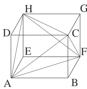
Example 2: Assume that the demands in Example 1 is bounded in a parallelepiped, namely w−_i ≤wi≤w+_i , i=1,2,3.

This box belongs to the subspace wi=0, i=4,5,6, then the

relative dimension is p=3,. Such a box can be partitioned in 4 simplices as in Fig. 2 (precisely (A–C–D–H), (A–C–F– H), (A–B–C–F) and (H–C–G–F)). Denote by ΦA . . .ΦH the

optimal values of u in problem (12) corresponding to w on the vertices wA. . .wH. Then the interpolating affine function

u=Φ(w) can be computed as follows. If, for instance, w is in the sector (A–C–D–H), then

Φ(w) =αAΦA+αCΦC+αDΦD+αHΦH,

whereαA,αC,αD andαH are (uniquely) determined by

αAwA+αCwC+αDwD+αHwH = w,

αA+αC+αD+αH = 1.

Lemma 1 introduces the following theorem concerning the solution of the static version of Problem 1.

Theorem 1: The cost of (11) is

ΨS=max

k∈K Ψ(u

(k)_,w(k)_{). (14)}

3_{a simplex in IR}n _{is a polytope with n+1 vertices; its relative interior is}

the interior within the smallest subspace includingW; the dimension p≤n

of such a subspace is the relative dimension

B

E

F

H

G

C

D

[image:5.595.362.504.124.269.2]

A

Fig. 2. Partition of a cube in 4 simplices.

Proof: Since the w in the static problem (11) can always be set as a vertex w=w(k), it is obvious that ΨS≥

maxk∈K{Ψ(u(k),w(k))} (we remind that u(k) ∈U are the

optimal values).

We show now thatΨS≤maxk∈K{Ψ(u(k),w(k))}. Consider

any point w∈W _{also included in the jth simplex of}W_{, that}

is, w∈W_j. Then, denoting byK_j⊂K the subset of indices identifying the vertices ofW_j,

w=

∑

k∈K_j

αkw(k), c.c.αk.

Take u=ΦPWA(w), the piecewise-affine strategy (13). Then

Ψ(u,w) = Ψ

Ã

∑

k∈K_j

αku(k),

∑

k∈K_j

αkw(k)

!

≤

∑

k∈K_j

αk Ψ³u(k),w(k)

´

≤max

k∈K_j

n

Ψ³u(k),w(k)

´o

≤

max

k∈K

n

Ψ³u(k),w(k)´o,

with c.c. αk(t). Note that the last inequality compares the maximum over all vertices ofW_{j with the maximum over all}

vertices ofW_.

An immediate consequence of the above theorem is that the strategy ΦPWA(w) in (13) is min-max optimal for the static

problem (11) as it guarantees that

Ψ(ΦPWA(w),w)≤Ψ(ΦPWA(w(r)),w(r)) =Ψ(u(r),w(r)),

where w(r) is the worst demand. Note that this strategy is not unique since all the strategies in the set

Q = {Φ(w): BΦ(w) =w,

Ψ(Φ(w),w)≤Ψ(ΦPWA(w(r)),w(r)),∀w∈W}

(15) are min-max optimal for the static problem (11). In particular, the set Q includes the strategy

ΦSOPT(w) =arg min

u∈U{Ψ(u,w): Bu=w, ∀w∈

W_} (16)

Remark 2: Note that the u selected by (16) is determinis-tically optimal for the pure static problem only, in the sense thatΨ(ΦSOPT(w),w)≤Ψ(u,w)for all w∈W and u∈U, not

optimal for our problem. Both ΦSOPT(w) and ΦPWA(w) are

plays first” [3]), in the sense that the flow is taken as a function of w which, in turn, maximizes the cost Ψ(ΦSOPT(w),w) in

one of the vertices w(r). So an interpretation of our result is that to design a min-max optimal strategy off-line we can solve a max-min problem on-line, i.e., (find minimizing flow for given demand).

B. Main theorem

We are in a position to prove that the optimal min-max cost is equal in the three versions (9)-(11) of the Robust Problem. Basically we prove that the worst-case demand for the static problem, namely the value w(r)∈W _{on which the maximum}

(14) is assumed, is indeed the worst-case demand for the time-varying problem we are considering.

Theorem 2: The following equalities hold

ΨM=ΨML=ΨS. (17)

Furthermore, as the inf-sup optimal values are achieved with strategyΦPWA(w)in all the three problems (9), (10) and (11),

then ΨM, ΨML andΨS are min-max optimal values and the

static strategyΦPWA(w)is a min-max optimal strategy.

Proof: The proof splits in two parts.

Proof of the claim ΨML=ΨS. Let w(r)∈vert{W} the

worst-case demand for the static problem (11), and let u(r) the corresponding (optimal) flow. Let u=Φ(w)any arbitrary memoryless strategy. Assume that the demand is constant w(t)≡w(r) and let ˆu=Φ(w(r)). Since u and w are constant, the average cost is

Ψ(u¯,w(r)) =Ψ(uˆ,w¯(r))≥Ψ(u(r),w¯(r)) =ΨS

by construction, so we haveΨML≥ΨS.

We now prove ΨML≤ΨS. For arbitrary w(t) and u(t) =

ΦPWA(w(t)), consider the averages ¯uT =AvT[u] and ¯uT =

AvT[w]the associated cost is

Ψ(u¯T,w¯T) = (18)

Ψ

Ã

1 T

Z T

0 _k

∑

_∈K

αk(t)u(k)dt,1 T

Z T

0 _k

∑

_∈K

αk(t)w(k)dt

!

=

Ψ

Ã

∑

k∈K

u(k) 1 T

Z T

0 αk( t)dt,

∑

k∈K

w(k) 1 T

Z T

0 αk( t)dt

!

=

Ψ

Ã

∑

k∈K

u(k) αkˆ (T),

∑

k∈K

w(k) αkˆ (T) !

(19)

with c.c.αk(t). Note that in (19) the sums are extended to all vertices of W but, at each time, only the non-zero αk(t) are those associated with current “active simplex”W_j, i.e. the one for which w(t)∈W_{j. It is obvious that the numbers}

ˆ

αk(T) = 1

T Z T

0 αk( t)dt

are c.c.. Consider insideU _×W the polytope having vertices

³

u(k),w(k)

´

. Since Ψ is convex, it reaches the maximum on its vertices then for all T

Ψ(u¯T,w¯T)≤max k∈KΨ

³

u(k),w(k)´=ΨS. (20)

If we take the limit over an infinite horizon by continuity we have

Ψ(Av[u],Av[w])≤ΨS

or, which is the same, ΨML ≤ΨS and therefore we can

conclude thatΨML=ΨS.

Proof of the claim ΨM=ΨML. Memoryless strategies are

special cases of the strategies with memory, and cannot do any better, thusΨM≤ΨML. We only have to show thatΨM≥ΨML.

Again we assume that w(t)≡w(r)_{, the worst-case demand. The} optimal strategy is, again, to take u=u(r)_{. Indeed for each T} and any u(t)∈U

Ψµ1

T Z T

0

u(t)dt,1 T

Z T

0 w(r)dt

¶

= Ψ³AvT[u],w(r) ´

≥Ψ³u(r),w(r)´, (21)

where the last inequality comes from the fact that the average ¯

uT∈U and u(r)is optimal by construction. ThenΨM≥ΨS=

ΨMLand thereforeΨM=ΨML.

Remark 3: The minimizer in the Robust Problems (9)-(11) chooses strategies and not flows (the min is overΦ(·)and not u(·)) and this justifies the fact that, as the worst demand is on a vertex, then the optimal flowΦ turns out to be a function which interpolates the optimalvaluesu(r)=Φ(wr)associated with the vertices w(r). Clearly u(r) need not to be a vertex ofU_.

So far, we have assumed that the average values of the realization of w and the flow computed by the strategy Φ always exist. The following remark points out that we may drop such an assumption.

Remark 4: In view of (20), it is always possible to prove that

lim sup

T→∞

Ψ(AvT[u],AvT[w])≤ΨS.

Therefore if we rewrite the Robust Problem in the “lim-sup version” we achieve that

ΨLS=. min

Φ maxw∈W lim sup_T→∞Ψ(AvT[u],AvT[w]),

s.t. Φ(·,w(t))∈U_{, Bu=w}

is equal toΨS no matter which type of strategy is chosen.

The following remark generalizes the results of this section to the discrete-time case. It will turn useful later on when we study networks with buffers.

Remark 5: Theorem 2 still holds if we state problems (9) and (10) in discrete-time with t=0,1,2, . . ..

IV. THE CASE OF NETWORKS WITH BUFFERS

on. Then, the new formulation (Buffer problem) is identical to that of Problem 1 if we replace (9) by

ΨB = minΦmaxw(·) Ψ(Av[u],Av[w]) s.t. u(t) =Φ(·,x(t),w(t))∈U_{, ∀}t,

w(t)∈W_{, ∀t,}

˙

x(t) =Bu(t)−w(t), ∀t, x(t)∈X_{, ∀t,}

x(t)∈εX_{, ∀t≥tf for some tf >0,}

(22)

where the vector x(t)describes the buffer levels, the bounding set X _{is convex and compact and includes the origin as an}

interior point, and the arbitrarily small set εX_{, with} ε_>0,

is the set within which x must be driven in finite time. Henceforth, given a generic setA _⊆Rn_{and beingλ a positive}

scalar, we denote by λA _={λ_{a : a∈}A_{}. The strategies} Φ

considered are of the form

u(t) = Φ(ξ(t),x(t),w(t),t), ˙

ξ(t) = Φ_ξ(ξ(t),x(t),u(t),w(t),t), (23) again, with no restrictions of the type of domain of the variables. Before presenting the solution of problem (22), we need to discuss certain feasibility conditions for it and some technical assumptions for a “nice” description of the bounding sets X_.

Problem (22) is feasible if and only if the following condi-tion holds [14]

W _⊂int{BU_}, (24)

where int{BU_{}means the interior part of set B}U_{. The above}

condition is stronger than condition W _⊂BU considered in the first part of this work. We also assume, without restriction, that

0∈W and 0∈int{U_} (25)

(we can always apply a proper translation to meet this as-sumption). As an immediate consequence of (24)-(25), we can affirm that there exists a scalarσ>0 such that

W _⊂(1−σ){BU_}.

Regards to the description of the bounding setX_{, we assume}

the following

Assumption 3: There exists a gauge function ψ which is smooth for x6=0 and such that

X _{={x :}ψ_(x)≤1}.

Let us remind that gauge functions are positive definite, convex, and positively homogeneous of order 1, i.e., such that

ψ(ξx) =ξψ(x) for ξ ≥0 [22]. Special gauge functions ψ are kxk or more in general kFxk2p with F full column rank and integer p≥1. Note that norms of the typekFxk∞may be arbitrarily closely approximated bykFxk2pfor p large. Then, non-smooth polytopic sets of the form X _{={x : Fx≤¯1},}

where ¯1= [1 1. . .1]T _{defined by functions of the type} ψ(x) =max

k Fkx,

where Fkis the kth row of F, can be approximated by smooth

sets Xˆ _{defined by functions of the type}

ˆ

ψ(x) = "

∑

k

(max{Fkx,0})p #1/p

.

We are now in a position to establish the main result of this section which says that problem (22) is equivalent to problem (10) and therefore to problems (9) and (11). It is apparent that, given the presence of buffers and no constraints on the initial value x(0) of their levels, a strategy as in Definition 1 can solve problem (22),since buffer level feed-back is necessary. To this end, let us introduce the following definitions.

Definition 4: The strategy is of the pure feedback form if u(t) =Φ(·,x(t)), namely it requires no information about the current value of w(t). The strategy is of the memoryless pure feedback form if u(t) =Φ(x(t)), namely it is function only of the current value of the buffer levels x(t).

The following theorem states that there exist strategies with a simple structure that solve problem (22).

Theorem 3: The following property holds

ΨB=ΨML. (26)

Furthermore, min-max optimal strategies can be obtained either adding a memoryless pure feedback component to a static strategy, that isΦ(x(t),w(t)) =Φ1(w(t)) +Φ2(x(t)), or through a pure feedback strategyΦ(·,x(t)).4

Proof: We first prove (26) under the assumption that w(t)

is known on-line. To do this, consider the following strategy

u(t) =Φ(x(t),w(t)) =Φ1(w(t)) +Φ2(x(t)), for all t≥0,

whereΦ1(w(t))is any static strategy, for instanceΦPWA(w(t)),

which solves problem (10), andΦ2(x)is a stabilizing term that we define later on. Note that

BΦ1(w(t)) =w(t)∈(1−σ)BU

then if we substitute u(t)in the state equation in problem (22) we get

˙

x(t) =BΦ(x,w)−w(t) =BΦ2(x).

Now takeΦ2(x)equal to the continuous function

Φ2(x) =satσ[−B†x],

where B†is any right inverse of B and the saturation function is defined as follows

sat_σ[−B†x] =−λ(x)B†x,

with

λ(x)=. max{λ˜ ≥0 : −λ˜B†x∈σU_}.

Note that this assures that Φ(x,w) =Φ1(w) +Φ2(x)∈U. Since σU includes 0 as an interior point we have that the Lyapunov derivative ofψ is negative for x6=0. Indeed, since for gauge functions∇ψ(x)x=ψ(x)holds for x6=0, we have

˙

ψ(x) =∇ψ(x)BΦ2(x) =−∇ψ(x)BB†λ(x)x=−λ(x)ψ(x)<0

for x6=0. Therefore,

x(t)→0

4_{this means that on-line “who play first” between u and w does not make}

(see [14] for details). Note that this means that, by continuity,

Φ2(x(t)) converges to zero and thus it has zero mean. This also means that

Av[u(t)] =Av[Φ1(w(t))].

It remains to prove that this strategy solves problem (22). Consider the average

Av[u] = lim

T→∞

1 T

Z T

0

u(t)dt (27)

=lim

T→∞

1 T

Z T

0 Φ1(

w(t))dt+lim

T→∞

1 T

Z T

0 Φ2(

x(t))dt(28)

=lim T→∞ 1 T Z T 0

Φ1(w(t))dt+lim

T→∞

1 T

Z _θ

0

Φ2(x(t))dt(29)

=lim T→∞ 1 T Z T 0

Φ1(w(t)) =Av[Φ1(w(t))]. (30) Then by repeating exactly the same arguments of the previous section we have that the first part of the theorem is proved.

We now show that a pure feedback robust strategy u(t) = Φ(·,x(t)) exists, i.e., a robust strategy that does not require the knowledge of the current value of w(t). This can be done by sampling the system at small intervals. Actually, letτ>0 and consider the following equation

x(kτ) =x((k−1)τ) +B Z kτ

(k−1)τ

u(t)dt− Z kτ

(k−1)τ

w(t)dt. (31)

Let us now introduce the discrete-time variable z defined as

z(kτ) =x((k−1)τ) +B Z kτ

(k−1)τ

u(t)dt, (32)

equation (31) yields

z(kτ)−x(kτ) =

Z kτ

(k−1)τ

w(t)dt=. τwˆ(kτ),

where ˆw(kτ)∈W _{is the average demand in[(k−1)}τ_,kτ_{]. This}

means that we can derive the integral of w over [(k−1)τ,kτ]

by simply computing z(kτ)and measuring x(kτ).

The idea is now to apply a piecewise constant flow which takes on the following constant value within each sampling interval [kτ,(k+1)τ),

u(t) =_Φˆ_{(z(kτ),x(kτ)) =Φ}ˆ_{1(z(kτ),x(kτ)) +Φ}ˆ_2(z(kτ)),

kτ≤t<(k+1)τ,where ˆΦ1 is meant to compensate the past demand and ˆΦ2∈σU is a feedback action. In particular, the term ˆΦ1 is chosen in such a way that

τB ˆΦ1(z(kτ),x(kτ)) =τwˆ(kτ) =z(kτ)−x(kτ), u1∈(1−σ)U.

The above condition is satisfied by

ˆ

Φ1(z(k),x(k)) =Φ(wˆ(kτ)),

where Φ(w) is any memoryless strategy which solves prob-lem (10) in its discrete-time version as defined in Remark 5. We just have to assume that the demand values w(t) for t=0,1,2, . . . are equal to ˆw(kτ) for kτ=t. To specify the

term ˆΦ2∈σU, first note that the latter equation together with (32) yields

z((k+1)τ) = x(kτ) +τB ˆΦ(z(kτ),x(kτ))

= x(kτ) +τB ˆΦ1(z(kτ),x(kτ)) +τB ˆΦ2(z(kτ))

= z(kτ) +τB ˆΦ2(z(kτ)),

then, select ˆΦ2(z(kτ))according to

ˆ

Φ2(z(kτ)) =

½

arg min_u∈σU ψ(z(kτ) +τBu) if z6=0

0 if z=0 .

Note that if we useψ(z(kτ))as discrete-time Lyapunov func-tion, the condition 0∈int{U_{}guarantees that}ψ_(z(k+1)τ₎₋

ψ(z(k)τ)≤ −β <0 until the rest condition ψ(z(˜kτ)) =0 is reached for some large enough but finite ˜k. As a consequence x(kτ) =z(kτ)−τwˆ(kτ)is ultimately bounded in the set τW_.

By assumingτ small enough we can drive x(kτ)insideεX_.

Given this, since z(kτ) =0 for any k≥˜k, the feedback strategy ˆ

Φ2(z(kτ)) is equal to zero then Av[Φˆ2(z(kτ))] =0. Now, consider the average value of u(t)

Av[u] = (33)

= lim T→∞ 1 T Z T 0

u(t)dt= lim

K→∞

1 Kτ

K−1

∑

k=0 Z (k+1)τ

kτ

u(t)dt (34)

= lim K→∞ 1 K K−1

∑

k=0 ˆ

Φ1(z(k),x(k)) + lim

K→∞

1 K

K−1

∑

k=0 ˆ

Φ2(z(k)) (35)

= Av[_Φˆ_{1(z(k),x(k))]. (36)} We have just proved that we can choose a strategy such that Av[u] =Av[_Φˆ_{1] =Av[Φ]whereΦis a memoryless strategy} solution of problem (10). Then, according to Remark 5, we have that ΨB≤ΨML. It is left to prove that ΨB≥ΨML, or,

which is the same,ΨB≥ΨS. To do this, let us denote by w(r)

the worst demand of the static problem (11). Assuming that w(t)≡w(r), an optimal strategy for u is to take u(t)≡Φ1(w(r)) as already shown by equation (21) in the proof of Theorem 2.

Remark 6: In the developed theory we assumed that the time required for state measurements and flow computation is negligible. If these operations introduce a delay τd, we can provide a sample-data reformulation of the problem and our results still hold. In particular, we can guarantee practical stability within someε-ball with ε depending onτd.

V. DETERMINISTIC VERSUS MIN-MAX OPTIMALITY

In this section, we tackle the case where the demand is a generic one and not the worst one as formulated in the Deterministic Problem. In particular, we remind that we wish to find a strategy Φ(·,w(t)) that for any realization of the demand solves the problem

ΦD = minΦ Ψ(Av[u],Av[w])

s.t. u(t) =Φ(·,w(t))∈U_{, ∀}t, Bu(t) =w(t), ∀t,

w(t)∈W_{, ∀t.}

(37)

ΦSOPT(w(t)) are not deterministically optimal. In particular,

we find a strategy with memory that performs strictly better than the strategy ΦSOPT(w(t))∈Q as in (16) for a simple

counterexample where Ψ(Av[u]) is a function of Av[u] only and is positively homogeneous. Conversely we will present a theorem which shows that to achieve the deterministic optimality we must resort to strategies with memory, i.e. given by differential equations, notwithstanding the fact that our model is described by algebraic equations. We prove our results under the following assumption.

Assumption 4: FunctionΨdepends on Av[u]only and it is convex and positive semidefinite. Furthermore Ψ is continu-ously differentiable in all points u for whichΨ(u)>0. Before providing the counterexample and the theorem, we would like to provide the following comments about the previous assumption.

• Given any convex function which is positive semidefinite, we can always approximate it by a smooth one over an arbitrarily large compact set as we have seen in Section IV.

• The requirement that Ψ is a function only of u is not a restriction. Indeed, we can make Ψ implicitly depend on w by reviewing w as additional components of u as expressed below

Bu−u˜ = 0,

˜

u = w.

• We can generalize the cost in a significant way by translating u and considering costs that are positive semidefinite with respect to a nominal flow u0satisfying the nominal demand w0, namely of the form Ψ(u−u0). We consider a strategy with memory u(t) =Φ(ξ(t),w(t))

as in (23) where ξ(t)and the strategyΦ are defined as

ξ(t) = ½

u(0) t=0 1

t

Rt

0u(τ)dτ t>0

⇔ ξ˙(t) =−ξ(t) t +

u(t)

t ,

uG(t) =Φ(ξ(t),w(t)) =arg min

v∈U_{: Bv=w(t)}∇Ψ(ξ(t))v. (38)

As a first observation, note that the time derivative ofΨ(ξ(t)), for the current value of ξ(t), turns out to be

˙

Ψ(ξ(t)) =∇Ψ(ξ(t))ξ˙(t) =∇Ψ(ξ(t)) µ

−ξ(t) t +

u(t)

t

¶

.

therefore, uGis the point-wise minimizer of such a derivative.

The rationale of this choice is that it trivially holds AvT[u] = ξ(T)and therefore, at any time t, an approximationΨ(ξ(t))

of the costΨ(Av[u])is available. The approximation is based on the average up to time t rather than on the long run average. Now, we select a strategy that, at time t, chooses among all possible flows that balance the current demand w(t), the one that induces a maximum decrease for the approximated cost. We will refer to this strategy as the Gradient-based strategy (hence the G in ΦG).

In the case of a non-differentiable Ψ we would have to replace the Lyapunov derivative by the generalized derivative

D+Ψ(ξ(t)) = lim

dt→0+sup

Ψ(ξ(t))−Ψ(ξ(t−dt))

dt

at the price of a much harder exposition (see for instance [12]). We provide a simple example showing that the strategy (38) works better than the ΦSOPT(w(t)) which means that static

strategies may be min-max optimal but they are not determin-istically optimal in general.

co

Example 3: Let us consider the simple example proposed in [5], Example 7, with one node and two arcs. The system is described by

u1(t) +u2(t) =w(t)

with flow and demand subject to constraints −2≤u1≤3,

C

O

A

B

K

G

H

E

F

u

D

u

[image:9.595.323.547.288.462.2]

1 2

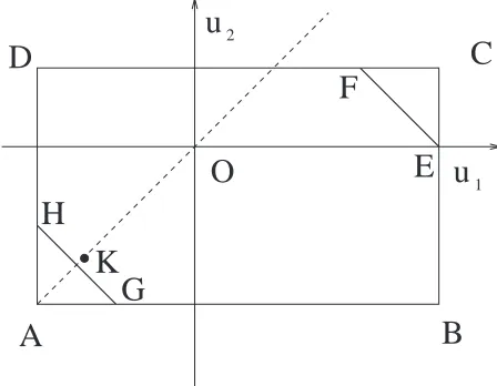
Fig. 3. Flow space of u1-u2 for the system of Example 3. The rectangle

A-B-C-D defines the setU_.

−2≤u2≤1 and |w| ≤2.8.

Figure 3 displays the flow space of u1and u2. The rectangle A-B-C-D defines the set U. Let the cost function be Ψ=

|Av[u1]−Av[u2]|, as we wish to have the same degree of long-term exploitation of u1 and u2. All points for which Ψ(·)is zero are described by the dashed line intersecting points A and O.

Consider a realization such that w(t) =2.8 for(2k)Θ≤t<

(2k+1)Θ and w(t) =−2.8 for (2k+1)Θ≤t<(2k+2)Θ, for some dwell timeΘ>0, k=0,1, . . .. In particular, as the realization is periodic, we can limit ourselves to study the evolution of the approximate cost in the first period (for k=0), the latter including the intervals 0≤t<Θ where w(t) =2.8 and Θ≤t<2Θ where w(t) =−2.8. We will show that in the first interval, we are not able to exploit the u1 and u2 at the same degree, as any feasible solution is such that u2 works harder than u1. In the second interval, the strategy (38) recovers the mismatch by initially letting u2 working harder than u1.

To be more precise, in the first interval, where w(t) =2.8, we must have u1+u2=2.8 (i.e., the segment E-F in Fig. 3) and strategy (38) returns u1=1 and u2=1.8 (i.e., the point F, which is the closest one to the dashed line u1=u2). During the interval functionΨ(ξ(t)) =0.8t and at the end of the first interval, for t=Θ, we haveΨ(ξ(t)) =0.8Θ.

returns u1=−2 and u2=−0.8 (i.e., the point H) in order to drive the approximate cost to zero as fastest as possible. Let ¯t be the first instant where Ψ(ξ(t)) =0. We have that for

Θ≤t<¯t, the functionΨ(ξ(t)) =0.8Θ−1_t.2(t−Θ). If we impose

Ψ(ξ(t)) =0 in the latter equation we find ¯t= 5

3Θ. In the remaining interval, namely for ¯t≤t<2Θ, the function takes on the valueΨ(ξ(t)) =0 and the strategy (38) switches to the flow u1=u2=−7₅ (point K).

As in t =2Θ, Ψ(ξ(t)) =0 the above reasoning can be applied for k=1 and so on. We have proved that Ψ(ξ(t))

is bounded, 0≤Ψ(ξ(t))≤ 0.8

t Θ for all t≥0. This means

that Ψ(ξ(t))→0 for t→∞. Since, Ψ(ξ(t))→Ψ(Av[u])also holds, we have shown thatΨ(Av[u]) =0 and then the strategy (38) is deterministically optimal for this example. Conversely, the cost associated to ΦSOPT(w(t)) is strictly greater than

zero which means that ΦSOPT(w(t)) is not deterministically

optimal. Actually, when w(t) =2.8, the strategyΦSOPT(w(t))

returns u1=1 and u2=1.8 (i.e., the point F), whereas when w(t) =−2.8, the strategyΦSOPT(w(t))returns u1=−1.4 and u2=−1.4 (i.e., the point K). On the average we have

Av[u1] =−0.2, Av[u2] =0.2, Φ(Av[u1],Av[u2]) =0.4. The deterministic optimality of (38) is proven next.

Theorem 4: Assume thatΨsatisfies Assumption 4. Assume that the gradient-based strategy (38) produces the average ¯uG=

Av[uG]. Let ˆu the average achieved by some arbitrary strategy

such that Bu(t) =w(t)for all t. Then

Ψ(u¯G)≤Ψ(uˆ).

Proof: To prove that Ψ(u¯G)≤Ψ(uˆ), we first note that

if Ψ(u¯G) =0 the result is straightforward sinceΨ is positive

semidefinite. Therefore assume Ψ(u¯G)>0. Denote by ξG(t)

the evolution of the integral variable with the gradient-based strategy. Since uG is the minimizer we must have

∇Ψ(ξG(t))u(t)≥∇Ψ(ξG(t))uG(t) (39)

for any other u(t)∈U such that Bu(t) =w(t).

Assume, by contradiction, that there exists a strategy u(t)∈

U _{such that Bu(t) =w(t)and that}Ψ_(uˆ)<Ψ_{(u¯G). Since}Ψ_is

convex, there exists β′>0 such that

∇Ψ(u¯G)[uˆ−u¯G]<−β′. (40)

Since ¯u=Av[uG]and ˆu=Av[u]are the average values, so that

Av[u−uG] =uˆ−u it turns out that for any¯ τ>0, no matter

how large, and any 0<β<β′ there exists t≥τ such that

∇Ψ(u¯G)[u(t)−uG(t)]<−β. (41)

Consider now the expression

∇Ψ(ξG(t))u(t)

= ∇Ψ(ξG(t))uG(t) +∇Ψ(ξG(t)) (u(t)−uG(t)) = = ∇Ψ(ξG(t))uG(t) +∇Ψ(u¯G) (u(t)−uG(t))

| {z }

<−β fort≥τ

+ [∇Ψ(ξG(t))−∇Ψ(u¯G)] (u(t)−uG(t))

| {z }

→0

,

w1 w2 w3 u1 u2 u3 u4 . . . u10 u11 u12

LB 5 1 3 2 3 4 0 . . . 0 -20 -20

UB 7 4 7 7 10 6 20 . . . 20 20 20

TABLE I

LOWERBOUNDSLBANDUPPERBOUNDSUBOF DEMANDS AND FLOWS.

where the last terms goes to 0 in view of the continuity of∇Ψ and the boundedness of u and uG. Then for a proper t large

enough

∇Ψ(ξG(t))u(t)<∇Ψ(ξG(t))uG(t)

in contradiction with (39).

Remark 7: If Ψ is linear, then ∇Ψ(ξ(t)) is constant and therefore variable ξ does not play any role. Then we can consider the memoryless strategy suggested in [4] for linear costs.

Remark 8: Given the average Av[w] =w, the value¯

Ψmin= min

Bξ=w¯,ξ∈U Ψ(ξ) (42)

is a lower bound forΨ(Av[uG]). To see this, note that Av[uG]

always satisfies BAv[uG] =w as well as Av¯ [uG]∈U, and

therefore Av[uG]is a generic feasible solution of problem (42).

Also, by exploiting the definition of achievable flows in [5], we can say that if the minimizer of (42) is an achievable flow, then the lower bound Ψmin is tight in the sense that

Ψmin=Ψ(Av[uG]). Differently, if the minimizer of (42) is not

an achievable flow, thenΨminis not tight asΨmin<Ψ(Av[uG]).

Furthermore, if we assume that ¯w is known, then we can adopt the linear strategy u−uG=F(w−w¯)proposed [5].

Let us conclude with a brief comment on the case of network with buffers. In presence of buffers, we can achieve the same results discussed in this section. To see this, it suffices to split the strategy in two parts: the first part assuring stability and the second part deterministic optimality. Such a procedure has already been illustrated in Section IV and therefore it will not be further discussed here.

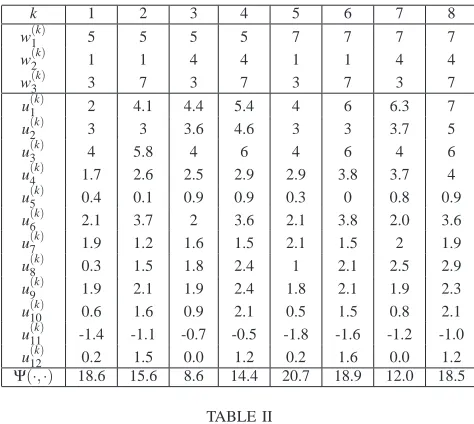
VI. NUMERICAL EXAMPLE AND SIMULATIONS

Consider again the network displayed in Fig. 1. We provide a comparison between the piecewise affine strategy (static min-max optimal strategy) ΦPWA(w) defined in (13) and

the gradient-based strategy (dynamic deterministically optimal strategy) uG(t) =Φ(ξ(t),w(t))as in (38). In Table I we display

lower and upper bounds of demands and flows.

The cost to minimize is (8) with ρ =0.1. Note that, we can make function Ψ(.) depend only on u as required in Assumption 4, by simply replacing demands w1(t), w2(t)and w3(t) by three artificial flows u13(t) =w1(t), u14(t) =w2(t) and u15(t) =w3(t). Table II summarizes the optimal balancing flows u(k)on each vertex w(k), k=1, . . . ,8. Observe that, from the network operator point of view, the cost Ψ(u(k),w(k)) is maximized in w(5). In other words, the worst demand is not the maximal demand on each node.

Now, denote pkthe probability of being on vertex w(k), and

k 1 2 3 4 5 6 7 8

w(₁k) 5 5 5 5 7 7 7 7

w(₂k) 1 1 4 4 1 1 4 4

w(₃k) 3 7 3 7 3 7 3 7

u(₁k) 2 4.1 4.4 5.4 4 6 6.3 7

u(₂k) 3 3 3.6 4.6 3 3 3.7 5

u(₃k) 4 5.8 4 6 4 6 4 6

u(₄k) 1.7 2.6 2.5 2.9 2.9 3.8 3.7 4

u(₅k) 0.4 0.1 0.9 0.9 0.3 0 0.8 0.9

u(₆k) 2.1 3.7 2 3.6 2.1 3.8 2.0 3.6

u(₇k) 1.9 1.2 1.6 1.5 2.1 1.5 2 1.9

u(₈k) 0.3 1.5 1.8 2.4 1 2.1 2.5 2.9

u(₉k) 1.9 2.1 1.9 2.4 1.8 2.1 1.9 2.3

u(₁₀k) 0.6 1.6 0.9 2.1 0.5 1.5 0.8 2.1

u(₁₁k) -1.4 -1.1 -0.7 -0.5 -1.8 -1.6 -1.2 -1.0

u(₁₂k) 0.2 1.5 0.0 1.2 0.2 1.6 0.0 1.2

[image:11.595.54.291.128.340.2]

Ψ(·,·) 18.6 15.6 8.6 14.4 20.7 18.9 12.0 18.5 TABLE II

OPTIMAL FLOWSu(k)_{ON EACH VERTEXw}(k)_{, k=1, . . . ,8.}

p5 0.2 0.4 0.6 0.8 0.95 1

ΨPWA−ΨG 4.5 5.5 5.3 4.3 1.6 0

TABLE III

COST DIFFERENCEΨPWA−ΨGFOR REALIZATIONS WITH DIFFERENTp5.

FORp5=1 (WORST REALIZATION),THE COST DIFFERENCE IS NULL.

Also, let ΨPWA=Ψ(Av[ΦPWA(w)]) and ΨG=Ψ(Av[uG]) be

the average costs obtained with strategiesΦPWA(w)and uG(t)

respectively. For this example, we can compute ΨPWA(w) =

∑8

k=1pkΨ(u(k),w(k))and deriveΨG by simulations. In

partic-ular, we simulate a set of six realizations for t from 0 to 500, with p₅=0.2,0.4,0.6,0.8,0.95,1. Whichever the realization, we expect a better performance of (38) as evidenced in Table III, where we display the cost difference ΨPWA−ΨG for

different realizations (different p5).

Note that in correspondence to the worst realization, char-acterized by p5=1, the two strategies ΦPWA(w) and uG(t)

are equivalently optimal asΨPWA−ΨG=0 (they provide the

same cost ΨPWA=ΨG=1).

Furthermore, according to our expectation, we observe that

Ψ(ξ(t))obtained with strategy (38) always converges toΨG

on the long run. This is evidenced in Figure 4 where we plot the time evolution of the error ∆Ψ(t):=Ψ(ξ(t))−ΨG for

each one of the six realizations. We can see that the error tends to zero for increasing t in all of the six plots. Note the straight line in zero which is associated to the worst realization (p5=1). In this case, the demand is the worst one at each t and∆Ψ(t) =0 which also meansΨ(ξ(t)) =ΨG=1 for all t.

Note that by using artificial flows u13(t), u14(t)and u15(t), the variableξ(t)includes also the average demands up to time t.

In Fig. 5, we simulate the gradient-based strategy uG(t)

defined in (38) (dotted) and the piece-wise strategyΦPWA(w)

defined in (13) (dashed) for a realization of the demand with p5=0.4. In particular, we plot flows ui(t)and demands wi(t)

0 50 100 150 200 250 300 350 400 450 500

−5 0 5 10 15 20

t

∆

Ψ

[image:11.595.323.549.131.307.2]

(t)

Fig. 4. Time plot of the error∆Ψ(t):=Ψ(ξ(t))−ΨG for a set of six

realizations with p5=0.2,0.4,0.6,0.8,0.95,1. The error tends to zero for

increasing t.

(solid) for i=1,2,3 from top to bottom respectively. Note that u2(t) obtained from the piecewise strategy (13) (dashed line, middle plot) follows the peaks of w2(t) (solid line, middle plot) while u3(t)does not. This is evident, for instance, in the interval from t=10 to t=15. This is due to the fact that arc 2 is over exploited for about t=8 where demand w2(t) =1 and the flow in arc 2 saturates at its lower value u2(t) =3. The gradient-based strategy uG(t) (38) keeps memory of the

mis-match between w2(t) and u2(t) and for t=10 to t=15 the flow u2(t)(dotted line, middle) is kept constant even if the demand w2(t)has some peaks at its highest value.

0 5 10 15 20 25

0 2 4 6 8

0 5 10 15 20 25

0 2 4 6 8

uG

(t), w(t)

0 5 10 15 20 25

0 2 4 6 8

t

Fig. 5. Gradient-based strategy uG(t)(38) (dotted) and piece-wise strategy

ΦPWA(w)(13) (dashed) with p5=0.4. Top: time plot of w1(t)(solid) and

u1(t)obtained with the gradient-based strategy uG(t)(dotted) and with the

piece-wise strategyΦPWA(w)(dashed); middle: time plot of w2(t)(solid) and

u2(t)(dotted and dashed); bottom: time plot of w3(t)(solid) and u3(t)(dotted

and dashed).

[image:11.595.320.555.525.721.2]

Network flows have been dealt with under different per-spectives both in robust optimization and in control theory. The present work is an attempt to emphasize connections and analogies between the two contexts.

We have studied how to robust stabilize continuous-time networks controlling flows with capacity constraints in the presence of demand which unknown but bounded within a polytope. A feature of this work is that the cost is a function of the long-run average-flow and demand. We have seen that assuming for the demand a worst or a neutral behavior leads to different optimal strategies. In particular, in the first case the resulting strategy is memoryless and can be computed via convex optimization. On the contrary, in the second case we must resort to strategies with memory.We have proposed a solution based on a Lyapunov approach, in which the control is selected on–line, among the feasible flows, as the point–wise minimizer of the gradient of the cost of the average.

REFERENCES

[1] E. Adida and G. Perakis, “A Robust Optimization Approach to Dynamic Pricing and Inventory Control with no Backorders”, Mathematical

Pro-gramming, Ser. B, vol. 107, 2006, pp. 97–129.

[2] A. Atamturk and M. Zhang, “Two–stage robust network flow and design under demand uncertainty” Operations Research, vol. 55, no. 4, 2007, pp. 662–673.

[3] T. Basar and G.J. Olsder, Dynamic Noncooperative Game Theory, SIAM, 1999.

[4] D. Bauso, F. Blanchini, and R. Pesenti, “Average Flow Constraints and Stabilizability in Uncertain Production-Distribution Systems”,

Proceed-ings of the American Control Conference 2007, New York, USA, 2007,

also submitted in an extended form to JOTA.

[5] D. Bauso, F. Blanchini, and R. Pesenti, “Robust control policies for multi-inventory systems with average flow constraints”, Automatica, Special Issue on Optimal Control Applications to Management Sciences, vol. 42, no. 8, 2006, pp. 1255–1266.

[6] A. Ben-Tal, L. El Ghaoui, and A. Nemirovski, “Foreword: special issue on robust optimization”, Mathematical Programming, Ser. B, vol. 107, 2006, pp. 1–3.

[7] A. Bemporad, F. Borrelli, and M. Morari, “Min-max Control of Con-strained Uncertain Discrete-Time Linear Systems”, IEEE Transactions

on Automatic Control, vol. 48, 2003, no. 9, pp. 1600–1606.

[8] D. P. Bertsekas and I. B. Rhodes, “On the Minimax Reachability of Target Set and Target Tubes”, Automatica, vol. 7, 1971, pp. 233-247. [9] D. P. Bertsekas “Linear Convex Stochastic Control problems over an

Infinite Horizon”, IEEE Transactions on Automatic Control, Dec. 1973, pp. 314–315.

[10] D. Bertsimas and A. Thiele, “A Robust Optimization Approach to Inventory Theory ”, Operations Research, vol. 54, no. 1, 2006, pp. 150– 168.

[11] D. Bertsimas, C. Caramanis, “Finite adaptability in mul-tistage linear optimization”, submitted, available as PDF at http://users.ece.utexas.edu/ cmcaram/.

[12] F. Blanchini, and S. Miani, Set-Theoretic Methods in Control, Birkh¨auser 2008, ISBN: 978-0-8176-3255-7.

[13] F. Blanchini, S. Miani, and F. Rinaldi, “Guaranteed cost control for multi–inventory systems with uncertain demand”, Automatica, vol. 40, no. 2, 2004, pp. 213–224.

[14] F. Blanchini, S. Miani, and W. Ukovich, “Control of production-distribution systems with unknown inputs and system failures” IEEE

Transactions on Automatic Control, vol. 45, no. 6, 2000, pp. 1072–1081.

[15] F. Blanchini, F. Rinaldi, W. Ukovich, “A network design problem for a distribution system with uncertain demand”, SIAM Journal on

Optimization, vol. 7, 1997, pp. 560-578.

[16] F. Blanchini, F. Rinaldi, W. Ukovich, “Least Inventory Control of Multi-Storage Systems with Non-Stochastic Unknown Input”, IEEE Transaction

on Robotics and Automation, vol. 13, 1997, pp. 633–645.

[17] E. K. Boukas, H. Yang, and Q. Zhang, “Minimax production planning in failure–prone manufacturing systems” Journal of Optimization Theory

and Applications, vol. 82, no. 2, 1995, pp. 269–286.

[18] A. Erera, J. Morales, and M. W. P. Savelsbergh, “Robust Optimization for Empty Repositioning Problems”, Operations Research, to appear, available at http://www2.isye.gatech.edu/˜mwps/publications/

[19] E. Khmelnitsky and M. Tzur, “Parallelism of continuous- and discrete-time production planning problems”, IIE Transactions, vol. 36, 2004, pp. 611–628.

[20] B. Grunbaum. Convex Polytopes, Wiley, New York, NY, 1967. [21] O. Kostyukova and E. Kostina, “Robust optimal feedback for

termi-nal linear-quadratic control problems under disturbances”, Mathematical

Programming, Ser. B vol. 107, 2006, pp. 131–153.

[22] D. Luenberger, Optimization via vector spaces methods, John Wiley & Sons, 1997.

[23] S. Mudchanatongsuk, F. Ord´o˜nez, and J. Liu, “Robust Solutions for Network Design under Transportation Cost and Demand Uncertainty”,

Journal of the Operational Research Society, vol. 59, 2008, pp. 652–662.

[24] F. Ord´o˜nez and J. Zhao, “Robust capacity expansion of network flow”,

Network, vol. 38, 2007, pp. 136–145.

[25] E.A. Silver and R. Peterson, Decision System for Inventory Management

and Production Planning. Wiley, New York, N.Y., 1985.

[26] S. Sethi, H. Zhang, and Q. Zang, Average cost control of stochastic