A new R function for the Internal External Uncertainty (IEU) model
Rachel K. Smedley
1∗1Department of Geography and Earth Sciences, Aberystwyth University, Ceredigion, SY23 3DB, UK
∗E-mail: [email protected]
Received: March 24, 2015; in final form: May 26, 2015
Abstract
A new function (calc IEU) is now available in the latest version of the R Luminescence package (version 0.4.2). Thecalc IEUfunction can be used to calculate an equivalent dose (De)
value for a given dose distribution using the Internal External Uncertainty (IEU) model. The IEU model is used in luminescence dating to determine a Devalue for a partially-bleached
sample by calculating the weighted mean from the well bleached part of a partially-bleached population. The new calc IEU function au-tomates the calculation of the IEU model so that the results are produced rapidly and reproducibly. This is advantageous as the user can easily perform sensitivity tests of the model in response to changing input parameters.
Keywords: R, luminescence dating, Inter-nal ExterInter-nal Uncertainty (IEU) model, single grains
1. Introduction
The Internal External Uncertainty (IEU) model can be used to determine an equivalent dose (De) value for
lumines-cence dating of a partially-bleached sample (Thomsen et al.,
2007). The Devalue is calculated as the weighted mean from
the grains in a partially-bleached population that the IEU model identifies to have been well bleached upon deposition. The IEU model has been successfully used in a number of studies to provide Devalues for sedimentary samples using
both single grains and multiple grains (e.g.Reimann et al.,
2012;Medialdea et al.,2014;Sim et al.,2014). A new func-tion that automates the calculafunc-tion of the IEU Devalue is now
available in the latest version of the R Luminescence package (version 0.4.2;Kreutzer et al.,2012). Thecalc IEUfunction
aims to automate the calculations of the IEU model for lumi-nescence dating, in addition to providing output features that rapidly assess the sensitivity of the IEU model to changing input parameters. The purpose of this work is to explain the calculations of thecalc IEU function and provide a worked example of the function using Devalues determined for
sin-gle grains of quartz from a glaciofluvial sample taken from the U.K. that was partially bleached upon deposition (sample T4CEIF01; Fig. 1a).
2. The IEU model
The IEU model is based on the assumption that the well-bleached grain population in the dose distribution from a poorly-bleached sample is normally distributed, and that this population can be identified if the uncertainties assigned to individual dose estimates adequately describe the observed variability. It is standard practise to determine the uncer-tainties on individual De values from intrinsic sources (i.e.
counting statistics, the instrument reproducibility and the dose-response curve fitting). Extrinsic factors such as hetero-geneity of the beta dose-rate for individual grains may also cause variability in a dataset. Ideally, the uncertainty aris-ing extrinsically for a given suite of samples is determined from a sample that has been well bleached in the natural en-vironment, meaning that factors such as microdosimetry are considered within the uncertainty estimate. However, it is often difficult to determine this information for all samples due to the lack of analogue well-bleached sediments in cer-tain depositional settings (e.g. glaciofluvial). Alternatively,
Thomsen et al.(2007) use a number of gamma dose-recovery experiments, administering progressively larger given doses to measure the minimal amount of scatter expected in a well-bleached Dedistribution. The authors plot the absolute
overdispersion values (in Gy) determined from these experi-ments against the CAM Devalues and fit a linear function to
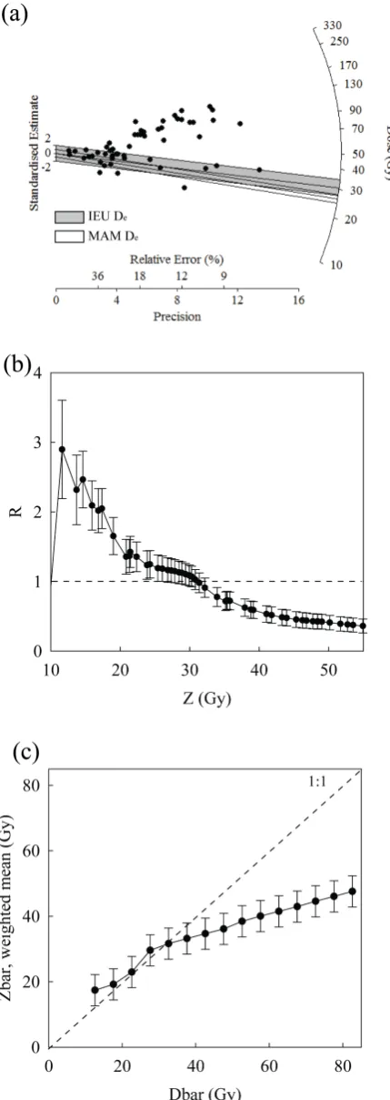
in-Figure 1. Results from applying the IEU model to Devalues
deter-mined from single grains of quartz from a partially-bleached sample taken from a glaciofluvial setting in the U.K. (sample T4CEIF01): (a) the Devalues are presented in a radial plot; (b) the values ofR
calculated for the final iteration ofDbarwhen determining the IEU Devalue for this dataset are plotted against Z; and (c) the output
plot from calculatingZbarusing fixed values ofDbarwhen a = 0.3
creasing given dose. In the IEU model the slope of this linear function is termed theavalue, which by definition is similar to theσb value in the Minimum Age Model (MAM; Gal-braith et al.,1999), while the intercept provides thebvalue, which defines how much overdispersion is expected in a De
distribution for a 0 Gy dose (e.g. the absolute overdispersion which can be obtained from thermal transfer experiments).
The uncertainty on each individual Devalue can then be
calculated using the uncertainty arising from counting statis-tics (σc2), thea andbvalues, and the burial dose (Dbar) in Eq. 1 (Thomsen et al.,2007).
σtot=
q
σc2+ (a·Dbar+b)2 (1)
The value ofDbarin Eq. 1 is initially unknown and so
Thomsen et al.(2007) suggest that it should be solved using an iterative approach. To iterateDbar, an initialDbarvalue is substituted into Eq. 1, and the total uncertainty assigned to each Devalue is calculated (σtot). The internal/external
con-sistency criterion (Eqs. 2, 3 and 4) is then used to determine which grains (or aliquots) from the partially-bleached popu-lation were well bleached upon deposition (Thomsen et al.,
2003). The weighted mean dose (termed Z) of the identi-fied well-bleached part of the partially-bleached population is then calculated and compared to the value ofDbar. IfZ is not equal toDbar, the calculation ofZ is repeated again using a new value of Dbar. This iteration process is con-tinued untilZis equal toDbar, whereZis calculated using only the grains (or aliquots) that are deemed to form the well-bleached part of the partially-well-bleached distribution (i.e. R= 1, see below). This value ofZ that is equal toDbaris the burial dose determined for this sample (termed the IEU De
value in thecalc IEUfunction).
To calculate the internal/external consistency criterion the De values in a given distribution are first ranked from the
smallest Devalue to the largest Devalue. Eq. 2 is then used to
calculate the weighted mean (Z), whereDiare the individual
Devalues,σi are the individual estimates of uncertainty for DiandNis the total number ofDi.
Z =∑
N
i=1Di/σi2
∑Ni=11/σi2
(2)
The standard error ofZis then calculated in two ways: (1) as an internal measure (α2in) which is dependent upon how
much variation there is within the counting statistics (Eq. 3); and (2) as an external measure (α2ex) which also is
depen-dent upon how much variation arises from each individual Deestimate varying from the mean (Eq. 4) (Topping,1955; Thomsen et al.,2003).
αin2 = 1
∑Ni=11/σi2
(3)
αex2 = ∑
N
i=1(Di−Z)2/σi2
(N−1)∑Ni=11/σi2
(4)
[image:2.595.61.276.72.677.2]uncertainty onRis(2(n – 1))-0.5andnis the number of data points used for the calculations.Ris calculated cumulatively, starting with the lowest two Devalues and finishing with
in-cluding all the Devalues into the calculation. All the grains
(or aliquots) included in the calculation of anR value≥1 are deemed to form the well bleached part of the partially-bleached population (e.g. Fig. 1b), andZis calculated from only these grains (or aliquots).
3. The
calc IEU
function: a worked example
Thecalc IEUfunction works in a similar way to the ex-isting age models built into the R ‘Luminescence’ package. It first requires the input of a data frame containing two columns; (1) the Devalues and (2) the uncertainties of the
Devalues. Input variables (or arguments) are also required
to define the parameters used for the calculations in the func-tion (e.g. a andb). The following section works through an example of how to use thecalc IEU function and what outputs are produced. Fig. 1a shows a radial plot containing the Devalues for the example dataset determined from
sin-gle grains of quartz from a glaciofluvial sample, which was partially bleached upon deposition. The individual estimates of uncertainty assigned to each De value shown in Fig. 1a
are based on counting statistics, instrument reproducibility (measured as 2.5 %) and dose-response curve fitting. Similar to theσbvalue in MAM, accurate estimates ofaandb
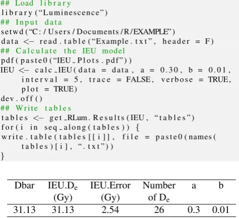
val-ues need to be considered for each sample. The uncertainty arising extrinsically for this sample was estimated from the overdispersion value determined for a sample from this en-vironment that was naturally well bleached upon deposition; aandbvalues for this sample were estimated to be 0.30 and 0.01, respectively. To call thecalc IEUfunction the user is required to adapt the arguments written below, defining the correct input parameters where necessary (e.g. aandb val-ues).
c a l c IEU ( d a t a = d a t a , a = 0 . 3 0 , b = 0 . 0 1 , i n t e r v a l = 5 , t r a c e = FALSE , v e r b o s e = TRUE , p l o t = TRUE )
data data.frame(required): containing two columns; Deand Deuncertainties
a numeric(required): slope (e.g. 0.30) b numeric(required): intercept (e.g. 0.01) interval numeric(required): interval used for fixed
iteration of Dbar (e.g. 5 Gy)
trace logical: print iteration of Dbar to screen (TRUE/FALSE)
verbose logical: console output (TRUE/FALSE) plot logical: plot output (TRUE/FALSE)
Before the IEU De value is determined for a De
distri-bution, thecalc IEUfunction will automatically calculateZ using fixed values of Dbarto assess whether there is more than one solution whereZ=Dbar(R= 1). Output plots of the results are provided to allow for comparisons if the user
wishes to compare the influence of changing input parameter (e.g. a) or the characteristics of Dedistributions determined
for different samples. Note that when performing the calcu-lations ofZusing a fixed value ofDbar,Z is referred to as Zbar to differentiate these calculations from the automatic iteration of Dbarused to calculate the IEU De value. The
fixed values ofDbarrange from an upper limit defined as the mean of the Dedistribution to a lower limit set as the lowest
Devalue in the dataset. Thecalc IEUfunction automatically
determines the fixed values ofDbarfrom the upper limit to the lower limit by repeatedly subtracting the value defined in Gy by the argumentinterval. The size of the interval used will depend on the range of the Dedistribution. If the range
in the Dedistribution is small then it would be advantageous
to use smaller intervals to improve the resolution of the cal-culations. The calculations from using fixed values ofDbar to calculateZbar are provided in an output table (e.g. Ta-ble 1), and the fixed values ofDbarare plotted againstZbar in an output plot (e.g. Fig. 1c).
Table 1 shows an example of what happens for the calcu-lations when using fixed values ofDbar. The mean is first calculated for the De distribution, here it is 82.59 Gy, the
fixed interval in Gy (i.e. 5 Gy) is then subtracted to deter-mine the firstDbar.fixedvalue of 77.59 Gy. ThisDbar.fixed value is then used to calculateR and determine how many grains form the well-bleached part of the Dedistribution. The
weighted mean (Zbar) of these grains is then calculated and plotted againstDbar.fixed(e.g. Fig. 1c). Thecalc IEU func-tion will then automatically subtract 5 Gy from the present value ofDbar(i.e. 77.59 Gy) to set a new value ofDbar.fixed (i.e. 72.59 Gy) used to calculate the next value ofZbar. This process continues to be repeated until the function identifies that the value ofDbar.fixedis set as a value lower than the lowest De value, whence the calc IEU function will cease
calculations.
The fixed iteration ofDbarin Fig. 1c demonstrates that there are multiple solutions ranging from 17.6 to 32.6 Gy whereDbar=Z andR= 1 for the example dataset used in this study, even though the final solution is determined to be (31.13±2.54) Gy (see Table 2). In such cases, the IEU De
value is the lowest value ofZthat is equal toDbar, because the model aims to determine a minimum dose from this De
distribution. Given that there may be multiple solutions of the IEU model for some data sets, it is important that the au-tomatic iteration ofDbarused to calculate the IEU Devalue
begins by setting the firstDbarvalue equal to the lowest De
value in the dataset and iterating to larger values of Dbar. Subsequent iterations ofDbarthen automatically setZ that was calculated during the previous iteration as the newDbar, and repeat the iterations untilDbar = ZwhereR= 1.
The argumenttraceallows the user to print the results to the screen from the iterations ofDbarto calculate the IEU Devalue. The calculations ofZ,α2ex,α2inandRused for
the final iteration ofDbarthat determines the IEU Devalue
Dbar Dbar.Fixed Zbar Zbar.Error n R a b
82.59 77.59 47.60 4.76 37 0.97 0.30 0.01
77.59 72.59 46.07 4.76 36 0.98 0.30 0.01
72.59 67.59 44.60 4.76 36 0.93 0.30 0.01
67.59 62.59 42.95 4.76 34 0.99 0.30 0.01
62.59 57.59 41.50 4.76 34 0.94 0.30 0.01
57.59 52.59 40.06 4.76 33 0.95 0.30 0.01
52.59 47.59 38.47 4.76 32 1.00 0.30 0.01
47.59 42.59 36.14 4.76 29 0.94 0.30 0.01
42.59 37.59 34.68 4.76 28 0.95 0.30 0.01
37.59 32.59 33.20 4.76 28 0.87 0.30 0.01
32.59 27.59 31.64 4.76 27 0.93 0.30 0.01
27.59 22.59 29.61 4.76 23 1.00 0.30 0.01
22.59 17.59 22.96 4.76 13 0.96 0.30 0.01
17.59 12.59 19.21 4.76 9 0.86 0.30 0.01
12.59 7.59 17.43 4.76 8 0.90 0.30 0.01
Table 1. Fixed iteration ofDbardetermined for the example dataset using anavalue of 0.30. The number of grains/aliquots determined to form the well-bleached part of the partially-bleached population is shown asn
file (e.g. Table 2), and contains the values forDbar, Z(now referred to as the IEU De), the uncertainty on the De value,
the number of De values defined as the well-bleached part
of the partially-bleached population, and theaandbvalues used for the calculations. For the example dataset given in Fig. 1a, the IEU Devalue (31.13 Gy±2.54 Gy) determined
using an avalue of 0.30 was consistent with the MAM De
value of (26.51 Gy±4.99 Gy), which was calculated using aσbvalue of 0.30 (Fig. 1a). An example of an R script that
a user can copy to call thecalc IEU function and save the output files is shown below (after Burow, Pers. Comm.).
# # Load l i b r a r y
l i b r a r y ( “ L u m i n e s c e n c e ” )
# # I n p u t d a t a
s e t w d ( “C : / U s e r s / Documents / R / EXAMPLE” )
d a t a <− r e a d . t a b l e ( “Example . t x t ” , h e a d e r = F )
# # C a l c u l a t e t h e IEU model
p d f ( p a s t e 0 ( “IEU P l o t s . p d f ” ) )
IEU<− c a l c IEU ( d a t a = d a t a , a = 0 . 3 0 , b = 0 . 0 1 , i n t e r v a l = 5 , t r a c e = FALSE , v e r b o s e = TRUE , p l o t = TRUE )
dev . o f f ( )
# # W r i t e t a b l e s
t a b l e s <− g e t RLum . R e s u l t s ( IEU , “ t a b l e s ” ) f o r ( i i n s e q a l o n g ( t a b l e s ) ) {
w r i t e . t a b l e ( t a b l e s [ [ i ] ] , f i l e = p a s t e 0 ( names ( t a b l e s ) [ i ] , “ . t x t ” ) )
}
Dbar IEU.De IEU.Error Number a b
(Gy) (Gy) of De
[image:4.595.50.287.454.670.2]31.13 31.13 2.54 26 0.3 0.01
Table 2. Results from calculating the IEU model for the example dataset shown in Fig. 1a.
Although it is not the case for the example dataset shown in this study, the IEU model may not always be able to deter-mine a Devalue using the input parameters provided, and an
error message will be produced by thecalc IEUfunction. It
is likely that an error message is provided because the popu-lation of grains that are deemed to form the well bleached part of the partially-bleached distribution is less scattered than can be explained by the value of a. In such cases, it is likely that the value of a is too large and overestimates the amount of scatter in a De distribution determined from
a well-bleached sample of this material; thus, the value ofa needs revising for the IEU model to be able to calculate a De
value for this sample.
4. Sensitivity of the IEU model to changing
pa-rameters
The outcome of any minimum age model that accounts for the uncertainties on individual Devalues (e.g. the IEU model
and MAM) is critically dependent upon the accuracy of the individual uncertainties assigned. Where the assigned uncer-tainties are overestimated, such a statistical model will over-estimate the number of grains that form the well-bleached part of the De distribution, and consequently overestimate
the Devalue. Similarly, if the assigned uncertainties are too
small then too few of the grains are determined to have been well-bleached upon deposition and the Devalue is
underes-timated. The uncertainties assigned to the individual De
es-timates must therefore be as accurate as possible in order to provide accurate Devalues for a given Dedistribution; this
includes using appropriate estimates ofaandbfor the IEU model.
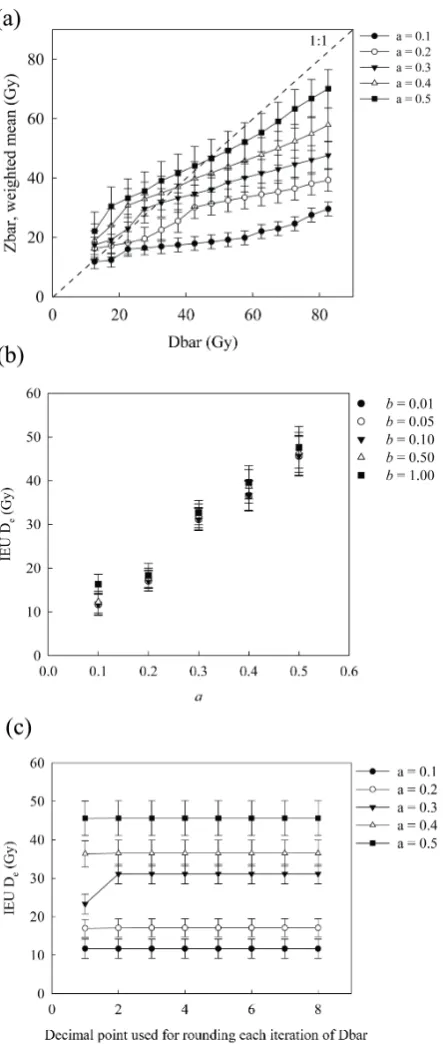
Figure 2. Results from applying the IEU model and changing differ-ent parameters for the example datasets: (a) fixed iteration ofDbar using a range ofavalues; (b) IEU Devalues calculated when
vary-ing both theaandbvalues; (c) IEU Devalues determined when the
values ofDbarandZare calculated to different decimal points for comparison using differentavalues.
sensitivity of the IEU Devalue to changing values ofacan be
different for Dedistributions determined from different
sam-ples (Medialdea et al.,2014;Sim et al.,2014). The example dataset (Fig. 1a) is used in this study to test how sensitive the IEU model is to varying the values ofaandb, and the
number of decimal points that the values ofDbarandZare calculated to for comparison. The results from performing fixed iterations ofDbarwhen changing theavalue from 0.1 to 0.5 are shown in Fig. 2a, and suggest that the fixed it-eration ofDbarusing ana value of 0.3 is the only dataset that has multiple solutions forDbar =Zbar. Fig. 2a plots the corresponding IEU De values calculated when
automat-ing the iteration ofDbarusingavalues from 0.1 to 0.5, in addition to simultaneously varying the value ofbfrom 0.01 to 1.00. These sensitivity experiments demonstrate that the IEU Devalue for this sample is highly sensitive to changes in
the value ofavalue but less sensitive to changes in the value ofb. This is because the value ofbonly becomes important for the calculations when the Dedistributions contain several
low Devalues, which is not the case for the sample shown in
Fig. 2. The differences in the IEU De values in Fig. 2
em-phasise the need to accurately quantify the amount of scatter in a naturally well-bleached Dedistribution for this material,
which is also an important requirement when applying the MAM.
The number of decimal points that the values ofDbarand Z are calculated to for comparison is also varied for the ex-ample dataset to assess whether this influenced the calcula-tion of the IEU Devalue (Fig. 2c). The results from varying
the number of decimal points from one to eight show how it did not affect the IEU Devalue for the majority of cases.
However, the IEU De value calculated using an avalue of
0.3 was lower whenDbarandZwere calculated to one deci-mal point (23.3 Gy±2.6 Gy), in comparison to when it was calculated to two decimal points (31.13 Gy±2.54 Gy). Al-though this is a very minor part of the calculations of the IEU model, Fig. 2c shows that it can have a large impact upon the Devalue determined. As a result, the calc IEUfunction is
designed to consistently calculate DbarandZ to two deci-mal points for comparison to ensure that all results are repro-ducible.
5. Conclusions
A new function (calc IEU) is now available in the R ‘Lu-minescence’ package and can be used to calculate burial dose estimates for a given De distribution. The IEU model can
be used to determine De values for luminescence dating of
partially-bleached samples by calculating the weighted mean from the grains of a partially-bleached population that were well bleached upon deposition (Thomsen et al.,2007). The calc IEU function is easy to use and rapidly automates the calculations. In addition to calculating the IEU Devalue, the
function uses fixed values ofDbaracross a range of the De
distribution to assess whether there is more than one solution for the model using the specified parameters. The efficiency of thecalc IEUfunction in calculating the IEU Devalue for
a dataset means that sensitivity tests of the model to chang-ing input parameters can be rapidly assessed. The sensitivity of the IEU De value to varying the amount of uncertainty
arising from the scatter in a naturally well-bleached De
ex-ample dataset in this study. The results demonstrate that the IEU Devalue for these data is highly sensitive to the value
ofa used. Performing sensitivity tests of the IEU Devalue
to parameters (e.g.a) can be particularly useful for lumines-cence dating of samples that are potentially complicated by additional sources of extrinsic uncertainty that are difficult to quantify (e.g. microdosimetry or bioturbation).
Acknowledgments
The author is grateful to K. Thomsen for checking the calculations performed in thecalc IEUfunction and for her insightful comments when reviewing this manuscript. C. Burow and S. Kreutzer are acknowledged for their contribu-tions in integrating the function into the R ‘Luminescence’ package. Thanks also to G. Duller for the problem solv-ing discussions dursolv-ing the writsolv-ing of parts of this function and to G. King and A. Stone for feedback on initial drafts of this manuscript. This paper was written while the author was supported by a Natural Environment Research Coun-cil consortium grant (BRITICE-CHRONO NE/J008672/1)), and the sample used as an example in this study (T4CEIF01) forms part of the BRITICE-CHRONO project.
References
Galbraith, R.F., Roberts, R.G., Laslett, G.M., Yoshida, H., and Ol-ley, J.M. Optical dating of single and multiple grains of quartz from Jinmium rock shelter, northern Austrailia: part I, experi-mental design and statistical models. Archaeometry, 41: 339– 364, 1999.
Kreutzer, S., Schmidt, C., Fuchs, M., Dietze, M., Fischer, M., and Fuchs, M. Introducing an R package for luminescence dating analysis. Ancient TL, 30: 1–8, 2012.
Medialdea, A., Thomsen, K.J., Murray, A.S., and Benito, G. Reli-ability of equivalent-dose determination and age models in the OSL dating of historical and modern palaeoflood sediments. Quaternary Geochronology, 22: 11–24, 2014.
Reimann, T., Thomsen, K.J., Jain, M., Murray, A.S., and Frechen, M.Single-grain dating of young sediment using the pIRIR signal from feldspar. Quaternary Geochronology, 11: 28–41, 2012.
Sim, A.K., Thomsen, K.J., Murray, A.S., Jacobsen, G., Drysdale, R., and Erskine, W. Dating recent floodplain sediments in the Hawkesbury-Nepean River system, eastern Australia using single-grain quartz OSL. Boreas, 43: 1–21, 2014.
Thomsen, K.J., Jain, M., Bøtter-Jensen, L., Murray, A.S., and Jungner, H. Variation with depth of dose distributions in sin-gle grains of quartz extracted from an irradiated concrete block. Radiation Measurements, 37: 315–321, 2003.
Thomsen, K.J., Murray, A.S., Bøtter-Jensen, L., and Kinahan, J. Determination of burial dose in incompletely bleached fluvial
samples using single grains of quartz. Radiation Measurements, 42: 370–379, 2007.
Topping, J.Errors of Observation and their treatment. The Institute of Physics and The Physical Society, London, 1955. pp. 91 93.