promoting access to White Rose research papers
White Rose Research Online
Universities of Leeds, Sheffield and York
http://eprints.whiterose.ac.uk/
This is an author produced version of a paper published in Ecological Modelling.
White Rose Research Online URL for this paper: http://eprints.whiterose.ac.uk/4129/
Published paper
Parry, H.R. and Evans, A.J. (2008) A comparative analysis of parallel processing and super-individual methods for improving the computational
performance of a large individual-based model, Ecological Modelling, Volume
Elsevier Editorial System(tm) for Ecological Modelling
Manuscript Draft
Manuscript Number: ECOMOD1606R1
Title: A comparative analysis of parallel processing and super-individual
methods for improving the computational performance of a large individual-based model
Article Type: Research Paper
Section/Category:
Keywords: Agent-based modelling; Individual-based modelling; Parallel computing; Super-individuals
Corresponding Author: Dr Hazel Ruth Parry, Ph.D.
Corresponding Author's Institution: Central Science Laboratory
First Author: Hazel Ruth Parry, Ph.D.
Order of Authors: Hazel Ruth Parry, Ph.D.; Andrew J Evans, Ph. D.
A comparative analysis of parallel processing
1
and super-individual methods for improving
2
the computational performance of a large
3
individual-based model
4
Hazel R. Parry
a,b,∗
, Andrew J. Evans
ba
b
School of Geography, University of Leeds, LS2 9JT, England
5
Abstract
6
Individual-based modelling approaches are being used to simulate larger complex
7
spatial systems in ecology and in other fields of research. Several novel model
de-8
velopment issues now face researchers: in particular how to simulate large
num-9
bers of individuals with high levels of complexity, given finite computing resources.
10
A case study of a spatially-explicit simulation of aphid population dynamics was
11
used to assess two strategies for coping with a large number of individuals: the use
12
of ‘super-individuals’ and parallel computing. Parallelisation of the model
main-13
tained the model structure and thus the simulation results were comparable to the
14
original model. However, the super-individual implementation of the model caused
15
significant changes to the model dynamics, both spatially and temporally. When
16
super-individuals represented more than around 10 individuals it became evident
17
that aggregate statistics generated from a super-individual model can hide more
18
detailed deviations from an individual-level model. Improvements in memory use
19
and model speed were perceived with both approaches. For the parallel approach,
20
significant speed-up was only achieved when more than five processors were used
21
and memory availability was only increased once five or more processors were used.
22
The super-individual approach has potential to improve model speed and memory
23
use dramatically, however this paper cautions the use of this approach for a
density-24
dependent spatially-explicit model, unless individual variability is better taken into
25
account.
26
Key words: Agent-based modelling, Individual-based modelling, Parallel
27
computing, Super-individuals
∗ Corresponding author. Address: Central Science Laboratory, Sand Hutton, York,
YO41 1LZ, England. Tel.: +44 1904 462724; Fax: +44 1904 462111.
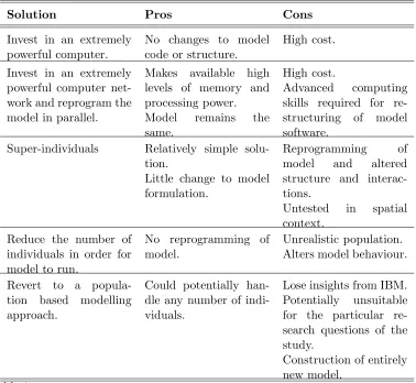
1 Introduction
29
A desire to better understand and inter-link the complex dynamic structures
30
of ecosystems, along with self-organisation, emergence of spatial and temporal
31
patterns and apparent unpredictability, has prompted a shift in the general
32
approach to ecological modelling today (Grimm and Railsback, 2005; Parrott
33
and Kok, 2000). Following trends in other fields of research, from social science
34
(Gilbert and Troitzsch, 1999) to fluvial sediment transport (Schmeeckle and
35
Nelson, 2003), there has been a shift away from procedural, equation-based
36
models to object-based simulations. These include individual-based models
37
(IBMs), cellular automata and multi-agent simulation (MAS). Such models
38
are concerned with modelling variation among individuals in a population,
39
and the interaction between individuals (DeAngelis and Gross, 1992; Grimm,
40
1999; Grimm and Railsback, 2005; Grimm et al., 1999; Huston et al., 1988;
41
Judson, 1994; Uchma´nski and Grimm, 1996). IBM is closely related to
multi-42
agent simulation. MAS has arisen from artificial intelligence (AI) research and
43
is used widely in other fields such as social science and computing (Gilbert
44
and Troitzsch, 1999).
45
Object-based approaches have been successfully implemented to model a range
46
of ecological systems (for a review see Grimm, 1999; Grimm and Railsback,
47
2005). They have the potential to further understanding of the local processes
48
that influence regional species population dynamics spatially and temporally,
49
enabling better understanding of how individual local-level and field-scale
in-50
teractions result in larger scale population distributions. However, some of
51
the potential of MAS and IBM methods is constrained by the demands that
52
may be placed on computing power. For realistic scenarios, it may be
essary to simulate large numbers of individuals. There may also be added
54
complexity, such as in models where interactions or agent-density are
impor-55
tant, but populations are sparse (for example insect populations, Parry et al.,
56
2006b, 2004), or where agents are memory-heavy because they are complex
57
(e.g. forest dynamics, Verzelen et al., 2006), or multiple types of agent are
58
used, such as in models of competition or predator-prey models (e.g.
Hos-59
seini, 2006). Haefner (1992: pp.156-157), with some foresight, identified future
60
developments in ecological individual-based models that would benefit from
61
advanced computing as: multi-species models; models of large numbers of
in-62
dividuals within a population; models with greater realism in the behavioural
63
and physiological mechanisms of movement; and models of individuals with
64
‘additional individual states’ (e.g. genetic variation).
65
The key limitations imposed by computer hardware are: (1) the number of
66
calculations that can be performed in a reasonable time (controlled by
pro-67
cessing power); (2) the number of agents that can be modelled (controlled
68
by memory). Relationships were determined between increasing numbers of
69
initial agents and the memory and simulation speed of a simple agent model
70
(described in section 2) run on a single 2.80 GHz Intel Xeon processor 2097 MB
71
RAM machine. Once the model is running, processor use of memory is nearly
72
linear and using an equation derived from the curve we can predict that at a
73
maximum available memory capacity of 1.5GB RAM on the single machine,
74
the theoretical limit to the initial number of agents is approximately 7,500,000.
75
However, at this limit, the simulation is calculated to take approximately 1
76
million seconds (12 days) to run (calculated from the simulation speed curve
77
using a quadratic function). This may be an under-estimate, as there is a
78
slight processing overhead for dealing with additional memory blocks, which
would result in a less linear relationship over time. The potential number of
80
replicates of a stochastic simulation are affected by this, so for example the
81
use of Monte Carlo techniques would no longer be possible.
82
There are a number of solutions to the problem of large numbers of
individu-83
als in an individual- or agent-based simulation (table 1). Solutions may range
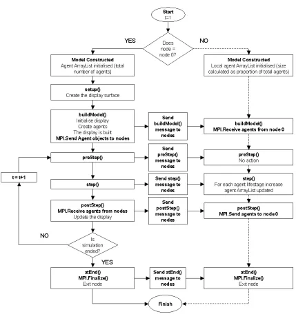
84
from hardware investment (such as obtaining a more powerful computer) to
85
computational solutions, such as changes in the software design (e.g.
paralleli-86
sation) or changes in the the model structure. This paper evaluates and
com-87
pares two such solutions to this problem. The first is a computational solution
88
that requires access to networked hardware: to parallel program the model
89
software to work across a network of powerful computers, so splitting the
pro-90
cessing/data load. The second is a mathematical solution, where the model
91
itself is altered so that individuals are aggregated into ‘super-individuals’
(af-92
ter Scheffer et al., 1995). The two methodologies are applied to a case study of
93
a spatially-explicit, individual-based simulation of aphid population
dynam-94
ics in agricultural landscapes (Parry et al., 2006b). The comparability of the
95
model results with the original model are first determined, then the two
ap-96
proaches are evaluated in terms of improved model efficiency (memory use
97
and speed).
98
A key advantage of parallel programming is that it maintains the strengths
99
of an individual-based approach whilst potentially increasing the number of
100
agents that can be simulated, as opposed to the super-individual approach
101
where the key interactions in the model are altered. However, parallelisation
102
is a complex solution, and although the agent interactions are unchanged
sig-103
nificant restructuring of the model software is needed. Haefner (1992) outlined
104
the potential applications of parallel computing to individual-based
tions in ecology, but also pointed out the need for ecological modellers to
106
improve their technical knowledge. Few examples of parallel simulations exist
107
in the ecological literature to date. Some examples of note are a parallel
sim-108
ulation of a school of fish by Lorek and Sonnenschein (1995) and several in
109
relation to the ATLSS project (http://atlss.org/), which include a parallel
110
individual-based model of Everglades deer ecology by Abbott et al. (1997) and
111
a parallel spatially-explicit fish model (ALFISH) by Wang et al. (2004). Other
112
agent simulation examples can be found outside ecology in the use of parallel
113
agents for reducing genetic algorithm search times (Lefley and McKew, 2004)
114
and performing large scale traffic simulations (Dupuis and Chopard, 2001).
115
The simplicity of the super-individual approach makes it attractive,
particu-116
larly as it does not require complex programming and powerful computer
sys-117
tems to implement. It maintains the philosophy and integrity of an
individual-118
based approach without reverting to a population model to deal with large
119
numbers of individuals. However, implementations of this approach to date
120
are primarily not spatially-explicit.
121
2 Application
122
The results presented in this paper relate to a simplified version of a spatially
123
explicit individual-based simulation model of aphid population dynamics in
124
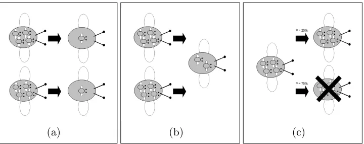
agricultural landscapes (Parry, 2006; Parry et al., 2006b, 2004). A
spatially-125
explicit IBM of aphid populations was constructed to assess the impact of
126
variation in agronomic practices in time and space. These practices included
127
crop introduction and configuration, pesticide spray application, matrix
habi-128
tat availability and fragmentation. The impacts that these have upon aphid
populations were observed, including both regional and local population
dy-130
namics as well as individual movement paths. A key limitation of the model
131
was the restriction on the number of insect agents that could be modelled.
132
The simplified model was used to explore and evaluate the options for
cop-133
ing with large numbers and complexity in the full model. The simple model
134
moves aphid agents (Rhopalosiphum padi) randomly from cell to cell around
135
a uniform landscape and local agent density is recorded. Aphids reproduce
136
parthogenetically with winged and non-winged morphs produced. Density
de-137
termines the proportion of alate (winged) morphs that are born at each
iter-138
ation. The simulation is begun with a population of alate agents originating
139
from a central cell in a 50×50 cell landscape, where each cell is 25×25 m. The
140
wind is set to a constant speed of 8kmh−1 and a constant westerly direction.
141
In the full version of the model there are a number of variables (some of which
142
are density dependent), realistic immigration across a region and a more
com-143
plex environment. The complexity of the full version of the model increases
144
computational demands beyond those demonstrated here and a large number
145
of agents (several million) were required for the simulation to be realistic at
146
the landscape scale.
147
Initial populations of 10, 100, 1,000, 10,000, 100,000 and 500,000 aphids were
148
used, originating from a single central cell. Each simulation was run thirty
149
times and an average taken to represent the total population trend over time
150
(as several parameters in the model are stochastic). While the model was
151
allowed to run for 120 days, spatial comparisons were made after 2, 20 and
152
40 days by creating surfaces that show the mean density in each cell over the
153
thirty runs. Temporal comparisons were made of the population dynamics at
154
the central cell.
3 Parallel computing
156
3.1 Implementation
157
In order to address computing problems where a model is hindered by data
158
requirements far larger than can be accommodated at any individual
pro-159
cessing element, parallel solutions are often implemented. The combined or
160
‘virtual shared’ RAM of several computers is used to cope with the amount of
161
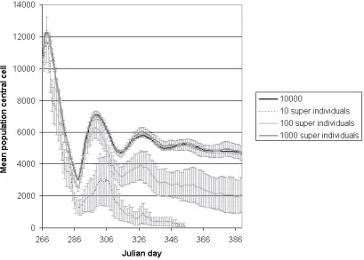
data and processing needed, using a Sequential-Algorithm Multiple-Data
ap-162
proach (SAMD), where the same algorithm is applied to different data items
163
on different processors (“nodes”). The scale of the problem for each
individ-164
ual computer is therefore reduced (often speeding the model up), or more
165
resources are made available (allowing for larger models). To parallelise the
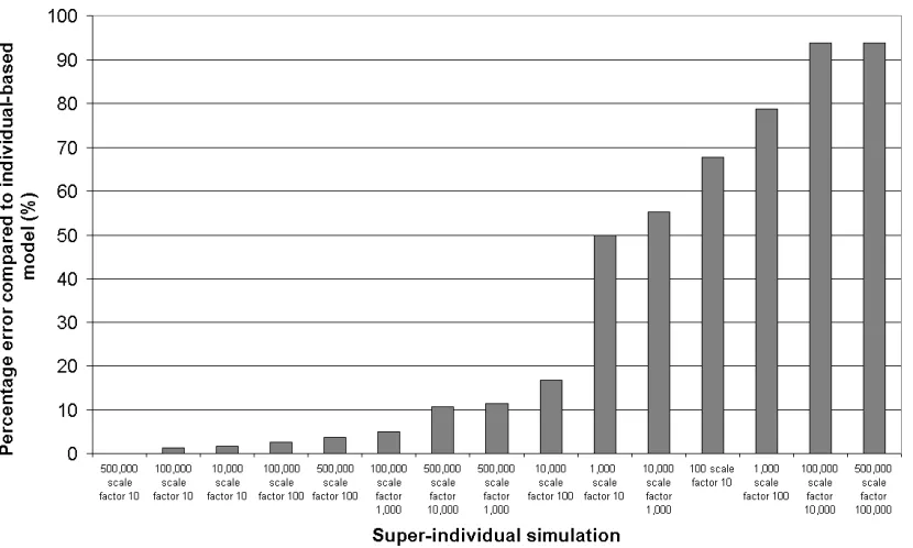
166
model software, sections are run on each node and then the nodes
periodi-167
cally communicate together to share results. This requires somewhat complex
168
communication strategies to make the physically distributed systems act as a
169
single unit.
170
Key to an efficient parallel model is minimising the inter-processor
communi-171
cations; it is these that take valuable time (Pacheco, 1997). Because of this,
172
in models with static agents that only interact locally it makes sense to divide
173
the environment and agents between processors. Conversely, in models with
174
roaming agents, it makes sense to divide up the agents and have a copy of the
175
whole environment on each processor. Hardest to deal with are the situations
176
where agents roam the environment, but also interact with each other. In such
177
cases dividing up either the agents or the environment results in an increase
178
in inter-processor messages or agent transfer.
In this case study, parallelisation essentially splits the agents in the simulation
180
between a number of processors (nodes), each containing information on the
181
environment and total agent densities. Direct agent interaction (to determine
182
morphology) is mediated by density in the model. Thus, aphids can be split
183
between processors because it is not necessary for each processor to know the
184
exact position of all the aphids, just the density within each section of the
185
environment on the other machines. This information can be collated at a
186
single ‘control’ node and the total densities broadcast to each ‘worker’ node.
187
The initial model was created using the agent-based simulation toolkit Repast
188
(http://repast.sourceforge.net). The toolkit was implemented in
paral-189
lel by running the Repast interface on the control node (including the GUI
190
etc.), while the rest of the model code is run independently on worker-nodes,
191
synchronised by the control node using message passing (Parry, 2006; Parry
192
et al., 2006a). Agents are established on the worker nodes, coordinated by
193
the control node. In coding the parallel version of the model software, the
194
same code is placed on each processor but different sections of code are run
195
dependent on the node ID. The code on the control node controls the model
196
input, output and program flow, using the standard Repast methods of ‘setup’,
197
‘buildModel’, ‘preStep’, ‘step’ and ‘postStep’ to structure the code and to
ini-198
tiate the simulation steps (figure 1). For example, when the method preStep
199
is run, the control node (node zero) is programmed to send out messages to
200
the other nodes to invoke agent methods associated with preStep (the model
201
is strongly synchronised). The updated agents pass density information back
202
to the control node when needed (figure 1). It was expected that the speed of
203
the simulation would increase with the number of nodes used, compensating
204
for any minor time delay caused by the timing control of the simulation from
the control node. A similar strategy was employed by Lorek and Sonnenschein
206
(1995) for a non-Repast simulation, which was found to increase simulation
207
speed as well as enable the size of the simulation to increase.
208
3.1.1 Message passing
209
The agent model was parallelised using a Message-Passing Interface (MPI)
210
for Java, MPIJava (http://www.hpjava.org), run on a 30-node distributed
211
memory parallel computer known as a Beowulf cluster. Message passing (MP)
212
is the principle manner by which Beowulf clusters are linked. MPIJava uses the
213
open-source native MPI ‘LAM’ (http://www.lam-mpi.org/). Further details
214
on the methods used to incorporate the MPI into the model are given in
215
Parry (2006); Parry et al. (2006a). The particular Beowulf cluster used for the
216
simulations presented here was a dedicated cluster of thirty machines (nodes),
217
where each node has dual 2.66 GHz Intel Xeon processors with 1280 MB of
218
DDR memory and 40GB 7200rpm internal IDE disks running over a switched
219
GB network. Although the results presented in this paper refer to simulations
220
conducted on a dedicated Beowulf cluster, the principles of parallelising the
221
model for a multi-core machine or a non-dedicated cluster would be very
222
similar. The model presented here has since been adapted to run on an Intranet
223
cluster of non-dedicated PCs and on a multi-core processor system without
224
re-coding the parallelisation, only altering the MPI commands in the code to
225
work with a customised MPI. Non-dedicated clusters of machines with mixed
226
specifications may however introduce problems of network unreliability and
227
performance bottlenecking on the slowest machines. Such issues are explored
228
further in Parry (in press).
3.1.2 Data mapping and load balancing
230
Data must be evenly distributed between the nodes, known as ‘load balancing’
231
(Pacheco, 1997). In this model, a balanced load was calculated using a form
232
of ‘block mapping’ (Pacheco, 1997). Agents were split evenly across the
sys-233
tem, whilst each node contained full environmental information. The agents
234
remained on the same node throughout the simulation, thus maintaining a
235
balanced load while being able to roam the environment. For all the parallel
236
simulations, it was found that the maximum memory used by each node was so
237
similar that 95% confidence limits derived from the standard error evaluated
238
to ±0.00 in all cases. This shows that the distribution of individuals across
239
the worker nodes was highly efficient, and the load very well balanced.
240
4 Super-individuals
241
4.1 Implementation
242
The super-individual approach to modelling large populations on an
individ-243
ual basis was proposed by Scheffer et al. (1995), comparable to the earlier
244
‘generalised individuals’ of Metz and de Roos (1992). A super-individual
ap-245
proach ‘allows zooming from a real individual-by-individual model to a cohort
246
representation or ultimately an all-animals-are-equal view without changing
247
the model formulation’ (Scheffer et al., 1995: pp. 161). The simple idea is that
248
individuals in a population can be grouped together into ‘super-individuals’,
249
thus reducing the number of objects to simulate and therefore reducing the
250
memory and processing power required (figure 2). For populations such as
251
aphids where there are high reproductive and mortality rates leading to large
juvenile populations, this approach can be very useful (Grimm and Railsback,
253
2005). It is possible to use the approach to test the effects of grouping
individ-254
uals, and also to examine the degree to which individual behaviour explains
255
the observed phenomena. A similar approach is used in physical models such
256
as the lattice models of fluid dynamics, particle modelling and Lagrangian
257
modelling (e.g. Woods and Barkmann, 1994).
258
4.1.1 Combining individuals into a single super-individual
259
Although Scheffer et al. (1995) state that no changes to the model
formula-260
tion are required for the super-individual approach, there are some significant
261
changes to the model structure that potentially influence the model results. To
262
convert the individual-based model to super-individuals, individuals
originat-263
ing at the same spatial location (cell) were split by initial age and morphology
264
(whether they have wings or not) into super-individuals. Each super-individual
265
represented a fixed number of individuals throughout the course of the
simu-266
lation.
267
4.1.2 Adding individual immigrants to super-individuals
268
Initial immigrants were added as super-individuals of the same scale factor
269
and, as in the unmodified model, these were of uniform age and morphology
270
(adult alates (i.e. winged)).
271
4.1.3 Mortality of individuals/super-individuals
272
Estimating the mortality of super-individuals can be done in a number of
273
ways, all of which are prone to error. The three main approaches are given by
Grimm and Railsback (2005: pp. 267) (figure 3):
275
N = the number of individuals represented by the super-individual (i.e. the
276
scale factor). N0= the number of individuals represented by the super-individual
277
at the start of the simulation.
278
(1) The number of super-individuals remains constant, and mortality reduces
279
N.
280
(2) N is kept relatively constant, by mortality reducing N until super-individuals
281
are recombined when N falls below N0/2.
282
(3) Assume that an entire super-individual dies when subject to mortality.
283
Both approaches 1 and 2 require dynamic updating of the number of
individ-284
uals represented by the super-individual, but in this way they do maintain
285
more of the original variability of the model. However, significant errors,
par-286
ticularly spatial errors, would be introduced as individuals are re-grouped,
287
and the process would be computationally intensive. Reducing the number of
288
super-individuals in approaches 2 and 3 has computational advantages (the
289
number of super-individuals to iterate is minimised and individual variability
290
is less important so calculations are less complex).
291
Approach 3 was chosen: super-individuals are subject to the same probability
292
of mortality as individuals and when the super-individual dies all individuals
293
represented by the super-individual die. This approach was chosen because
294
the variability between individuals of the model (particularly age) meant that
295
approach 2 (recombining individuals) was problematic. Approach 1
(main-296
taining a constant number of super-individuals) would also be problematic to
297
implement as the constant updating and variability of N would be
computa-298
tionally intensive, particularly as the density of individuals is important to a
number of model processes. Approach 3 was therefore considered to be the
300
most computationally efficient, although the least biologically realistic as it
301
suggests that mortality affects equally a group of aphids of uniform age and
302
morph in a particular cell (discretization of mortality). Another potential
is-303
sue with approach 3 is that it may require a lower value of N than the other
304
approaches to avoid excessive discretization of mortality. This paper assesses
305
whether this is the case.
306
4.1.4 Changes to the model structure
307
The construction of a super-individual simulation involved very little
alter-308
ation of the model structure (for details of this structure see Parry et al.,
309
2006b, 2004). A variable was added to record the number of individuals all
310
super-individuals actually represent. Equations that were dependent on
den-311
sity (such as morphology determination) were altered so that the density
val-312
ues were related to the real number of individuals in the simulation, not the
313
number of super-individuals (see equation 1). This was because the proportion
314
of alates produced is in relation to the density of individuals.
315
Morph determination is represented by the equation:
316
ALP ROP = 0.002 + 0.991
(1 +EX P(−0.076×(DEN SI T Y −67.416))) (1)
317
where ALPROP = the proportion of newly laid nymphs that will become alate
318
and DENSITY = the total number of individual aphids per plant.
319
5 Evaluation
321
The parallel version of the model produced extremely similar results to the
322
non-parallel model, as expected (no changes were made to the model structure,
323
only to the software). Variability between the original model and the parallel
324
model was only due to the model’s stochasticity. However, the super-individual
325
model did alter the model structure, therefore some variation was expected
326
in the output between the super-individual model and the original model.
327
This variability is presented first below, then a comparison is made of the
328
improvement in performance in terms of model speed and memory use for
329
both the parallel and super-individual approach in relation to the original
330
model.
331
5.1 Super-individual temporal and spatial replication of the individual-based
332
simulation
333
Movement of super-individuals followed the same rules as that of individuals,
334
however this produced spatial clustering of the populations. To test the
super-335
individual model, populations of 100, 1,000, 10,000 and 100,000 and 500,000
336
individuals were represented by varying numbers of super-individuals (Table
337
2). Results are compared to the original individual-based model, both
tem-338
porally and spatially, in the following sections. Results from simulations with
339
10,000 individuals are given in more detail as an example to demonstrate the
340
effects of combining individuals.
5.1.1 Temporal
342
Overall, for simulations of fewer than 10,000 individuals the super-individual
343
simulations produced population densities that were much lower than the
344
individual-based model equivalent (figure 4). For 10,000 individuals,
densi-345
ties only become significantly lower at the second population peak, and the
346
super-individual simulations also reach this peak earlier. This can be related
347
to the spatial results (below), where it is only after this point in time that
348
it is evident that differing spatial distributions and densities are beginning to
349
emerge. The only case where the super-individual simulation falls within the
350
95% confidence limits of the original model for the duration of the simulation
351
period is the simulation of 10,000 individuals with 1,000 super-individuals
352
(scale factor 10), figure 4. The percentage error between the temporal results
353
for all the super-individual simulations and the individual-based simulations is
354
shown graphically in figure 5. This confirms that super-individual simulations
355
of 10,000 aphids and above with low scale factors may be acceptable. This
356
also shows that when a large number of individuals are represented by very
357
few super-individuals (in this case 10 super-individuals) the error is greatest.
358
Excessive discretization of mortality is therefore evident (suggested in section
359
4.1), resulting in a need to reduce the scale factor for results to better represent
360
the individual-based model.
361
5.1.2 Spatial
362
Clustering is evident in the spatial distribution. The super-individuals are
363
contained in fewer cells, closer to the origin, than the individual-based
simu-364
lation. This is illustrated for 10,000 individuals by figure 6. The distribution
better replicates the unmodified model when the number of super-individuals
366
is maximised and the individuals they represent minimised, due to the
assump-367
tion that when mortality occurs, the whole super-individual dies. Only when
368
the number of individuals within the super-individual (N) is minimised in a
369
large population of super-individuals can this be overcome (Grimm and
Rails-370
back, 2005). However, even when this is the case, for 10,000 individuals with
371
1,000 super-individuals (scale factor 10) (figure 4) this still does not produce
372
a similar spatial distribution pattern, despite giving a satisfactory temporal
373
result. This suggests that errors in spatial distribution may be hidden in
super-374
individual models validated temporally. The super-individual patterns are in
375
fact most comparable to the patterns of the individuals for the same number,
376
e.g. 10 super-individuals compares well with the distribution of 10 individuals,
377
the difference is the density at each cell. This is the expected result when the
378
local redistribution of (super)individuals is the main process determining the
379
spatial distribution, despite density affecting morphology.
380
5.2 Speed
381
Super-individuals always improve the model speed (figure 7). The speed
im-382
provement is enormous for the largest simulations, where 500,000 individuals
383
simulated with super-individuals using a scale factor of 100,000 increases the
384
model speed by over 500 times the original speed. However, it was shown above
385
that only large simulations with a low scale factor (10-100) may benefit from
386
the super-individual approach, thus for these scale factors an improvement
387
in model speed of approximately 10,000-30,000% (100-300 times) the original
388
speed would result for simulations of 100,000 to 500,000 individuals.
Adding more processors does not necessarily increase the model speed.
Fig-390
ure 7 shows that for simulations run on two nodes (one control node, one
391
worker node) the simulation takes longer to run in parallel compared to the
392
non-parallel model. Message passing time delay and the modified structure of
393
the code are responsible. As the number of nodes used increases, the speed
394
improvement depends on the number of agents simulated. The largest
im-395
provement in comparison to the non-parallel model is when more than 500,000
396
agents are run across twenty-five nodes, although the parallel model is slower
397
by comparison for lower numbers of individuals. However, when only five nodes
398
are used the relationship is more complex: for 100,000 agents five nodes are
399
faster than the non-parallel model, but for 500,000 the non-parallel model is
400
faster. This is perhaps due to the balance between communication time
in-401
creasing as the number of nodes increases versus the decrease in time expected
402
by increasing the number of nodes. Overall, these results seem to suggest that
403
when memory is sufficient on a single processor, it is unlikely to ever be
effi-404
cient to parallelise the code.
405
5.3 Memory usage
406
Super-individuals always reduce the memory requirements of the simulation
407
(figure 8). The memory requirements for a simulation of super-individuals has
408
a similar memory requirement to that of an individual-based simulation with
409
the same number of agents. For simulations of 100,000 agents this can reduce
410
the memory requirement to less than 10% of the memory required for the
411
individual-based simulation with a scale factor of 10,000, and for simulations
412
of 500,000 agents this may be reduced to around 1% with the same scale
factor.
414
The mean maximum memory usage by each worker node in the parallel
simu-415
lations is significantly lower than the non-parallel model, for simulations using
416
more than two nodes (figure 8). The two node simulation used more memory
417
on the worker node than the non-parallel model when the simulation had
418
100,000 agents or above. This is probably due to the memory saved due to the
419
separation of the GUI onto the control node being over-ridden by the slight
420
additional memory requirements introduced by the density calculations.
How-421
ever, when 5 and 25 nodes are used, the memory requirements on each node
422
are very much reduced, below that of the super-individual approach in some
423
cases. The super-individual approach uses the least memory for 500,000
indi-424
viduals, apart from when only a scale factor of 10 is used (then the 25 node
425
parallel simulation is more memory efficient).
426
6 Discussion
427
The parallel model produced identical results to the initial model, as this
428
modifies only the model software and not the model itself. However, the
super-429
individual approach did not produce identical results to the initial model,
430
especially when assessed spatially. The similarity between the super-individual
431
results and the initial, unmodified model varied according the number of real
432
individuals that the super-individual was representing, and the number of
433
individuals simulated. The super-individual approach can only be considered
434
in situations where the number of individuals is high and the number of real
435
individuals represented by each super-individual is low (i.e. a low scale factor).
For the super-individual approach, within-cell density peaks vary temporally
437
between simulations run with different super-individual sizes. This is due to
438
the differences in emigration and movement patterns as a result of the size
439
of the super-individuals, as well as the method used to represent mortality.
440
Excessive discretization of mortality is evident as it is assumed that an
en-441
tire super-individual dies when subject to mortality. Further assessment of
442
the model (Parry, 2006) shows that regionally, the total population density is
443
similar between the different super-individual configurations and the
unmodi-444
fied model, but as shown in figure 6 there is a clear difference in the dispersal
445
patterns. Overall, the evidence indicates that the variability is such that the
446
super-individual approach is not suitable for the spatially-explicit simulation
447
of the aphid model, as presented here. Indeed, although the aphid model
448
is more strongly density dependent than most ecological models, most are
449
to some degree density dependent, rendering super-individual models
prob-450
lematic for spatially informative work. Modifications to the approach could
451
make it a possibility for future work. Experimentation with the other rules
452
for super-individual mortality suggested in section 4.1 would be a first step.
453
Other possible modifications include:
454
(1) Weighted kernels around a central ‘super-individual’, so that a more
re-455
alistic dispersal pattern is achieved.
456
(2) Relocation of a percentage of the super-individuals from a cell, without
457
actual population redistribution.
458
(3) Cell population model with individual migration.
459
However, re-distribution of individuals could significantly increase run-time,
460
adds complexity to the simulations and may take more memory than the
461
individual-based approach. This would also rely on a non-naturalistic model
of dispersion. Most movement in the model is a short distance each day, so
463
there will be constant shifting from super-individual to individual or creation
464
of dispersal kernels.
465
Further investigation may also indicate that spatial heterogeneity may have a
466
strong impact on the accuracy of the super-individual approach. The
simula-467
tions presented here were conducted in a neutral landscape, but if the model
468
were run in a heterogeneous landscape the interactions of the individuals with
469
the landscape may create model feedback that might further affect the
accu-470
racy of the super-individual results, both spatially and temporally.
471
Although the parallel solution appears to be more appropriate, in order to
en-472
sure it is optimised for agent simulations the balance between the advantage
473
of increasing the memory availability and the cost of communication between
474
nodes must be assessed in relation to the number of individuals simulated.
475
When the number of individuals is low, parallel simulations take longer
(fig-476
ure 7) and are less efficient (figure 8) than a non-parallel model run on a
477
single node. Increasing the number of nodes can reduce the demands on each
478
individual node, but time to communicate between processors may also be
479
increased (depending on the way in which the model is parallelised).
480
For the model presented here, estimates of the maximum number of agents
481
that can be simulated for varying numbers of nodes (table 3) and the
maxi-482
mum number of agents for a given super-individual scale factor (table 3) were
483
calculated with 1GB RAM, based upon information in figure 8. For the parallel
484
version, when only two nodes are used the non-parallel simulation is estimated
485
to have a higher maximum agent capacity per worker node, because space is
486
not being used by the message passing code. However, from five nodes and
up there is a higher maximum agent capacity for the parallel version than the
488
non-parallel model. The maximum agent capacity of 25 nodes is very high, at
489
nearly 100 million. This is approximately ten times the number of agents that
490
can be run within a reasonable time in the individual-based model. For low
491
numbers of nodes run times are huge: for two and five nodes the run times are
492
estimated to be 13 days and 47 days respectively. This would be expected to
493
increase with the complexity of the simulation. For any given model there will
494
be a threshold below which parallelisation is not efficient. Investigating this
495
threshold is likely to be a matter of iterative development as demonstrated
496
here, starting with a stripped-down model containing just the basic
message-497
passing elements. Passing of agents between nodes is processor intensive, and
498
therefore should be minimised. In this model, only the environment object
499
and information on the number of agents to create on each node are passed
500
from the control node to each of the nodes, and only density information is
501
returned to the control node for redistribution and display (see figure 1).
502
For the super-individuals (table 4) the relationship between the maximum
503
number of individuals that can be simulated and the scale factor is very simple.
504
The run time remains the same, as the maximum number of super-individuals
505
or individuals is constant. The maximum number of individuals that can be
506
simulated by this approach therefore depends purely on the scale factor used.
507
It would therefore not be unrealistic to assume this approach may potentially
508
enable the simulation of very large numbers of individuals indeed, in excess
509
of 7E11
if a scale factor of 1,000,000 is used, for example (assuming this scale
510
factor may be acceptable).
7 Conclusion
512
In order to address the limitations on the number of agents imposed by the
513
processing power and memory available, two solutions have been tested:
par-514
allel processing and super-individuals. The parallel approach involved
signifi-515
cant recoding of the model software, but no changes were made to the model
516
structure and performance increased significantly, enabling the simulation of
517
at least ten times more agents. The parallel model produced results that are
518
comparable to the initial, non-parallel model, leading to the conclusion that for
519
the simulation of very large populations the parallel model is a good solution.
520
Although initially far simpler to implement, the super-individual approach is
521
inappropriate for spatial simulations in the form presented here. However,
522
it may be possible to use this approach if the model were to be
signifi-523
cantly altered, by using another approach to simulate super-individual
mor-524
tality, or a super-individual model merged with an individual-based model,
525
where dispersal can be simulated by switching from a super-individual to an
526
individual-based model when necessary. There is a high risk that the
complex-527
ity of switching between model or implementing retrospective re-distribution
528
of agents could introduce significant error and put high demands on the
pro-529
cessor and/or memory, which are already limited. Overall, the results
pre-530
sented here indicate that the super-individual approach is inappropriate to
531
the spatially-explicit simulation of populations with density-dependent
func-532
tions or interactive agents, unless individual variability is better taken into
533
account. If this can be achieved satisfactorily, it has been demonstrated that
534
the super-individual approach may lead to very large reductions in
computa-535
tional demands.
8 Acknowledgements
537
This work is part of a PhD funded by the Central Science Laboratory
(De-538
fra Seedcorn). Thanks to Daniel Parry for his advice on Java programming
539
and Phil Northing and two anonymous reviewers for their comments on the
540
manuscript. The authors are members of the Multi-Agent Systems and
Simu-541
lation Research Group, School of Geography, University of Leeds.
542
References
543
Abbott, C. A., Berry, M. W., Comiskey, E. J., Gross, L. J., Luh, H.-K., 1997.
544
Parallel individual-based modeling of everglades deer ecology. IEEE
Com-545
putational Science and Engineering 4 (4), 60–78.
546
DeAngelis, D., Gross, L. (Eds.), 1992. Individual-based models and approaches
547
in ecology: populations, communities and ecosystems. Routledge, Chapman
548
and Hall, New York, 544 pp.
549
Dupuis, A., Chopard, B., 2001. Parallel simulation of traffic in Geneva using
550
cellular automata. Nova Science Publishers, Inc., Commack, NY, USA.
551
Gilbert, N., Troitzsch, K. G., 1999. Simulation for the Social Scientist. Open
552
University Press, Buckingham, 288 pp.
553
Grimm, V., 1999. Ten years of individual-based modelling in ecology: what
554
have we learned and what could we learn in the future? Ecological Modelling
555
115, 129–148.
556
Grimm, V., Railsback, S. F., 2005. Individual-based Modeling and Ecology.
557
Princeton Series in Theoretical and Computational Biology. Princeton
Uni-558
versity Press, Princeton, 480 pp.
559
Grimm, V., Wyszomirski, T., Aikman, D., Uchma´nski, J., 1999.
based modelling and ecological theory: synthesis of a workshop. Ecological
561
Modelling 115, 275–282.
562
Haefner, J. W., 1992. Parallel computers and individual-based models: An
563
overview. In: DeAngelis, D. L., Gross, L. J. (Eds.), Individual-based
mod-564
els and approaches in ecology: populations, communities and ecosystems.
565
Routledge, Chapman and Hall, New York, Ch. 7, pp. 126–164.
566
Hosseini, P. R., 2006. Pattern formation and individual-based models: The
567
importance of understanding individual-based movement. Ecological
Mod-568
elling 194 (4), 357–371.
569
Huston, M., DeAngelis, D., Post, W., 1988. New computer models unify
eco-570
logical theory. BioScience 38 (10), 682–691.
571
Judson, O., 1994. The rise of the individual-based model in ecology. Trends in
572
Ecology and Evolution 9, 9–14.
573
Lefley, M., McKew, I. D., 2004. Can a parallel agent approach to genetic
algo-574
rithms reduce search times. In: Loffi, A., Garobaldi, J. (Eds.), Applications
575
and Science in Soft Computing. New York: Cambridge University Press, pp.
576
69–74.
577
Lorek, H., Sonnenschein, M., 1995. Using parallel computers to simulate
578
individual-oriented models in ecology: a case study. In: Proceedings: ESM
579
’95 European Simulation Multiconference, Prague, June 1995.
580
Metz, J. A. J., de Roos, A. M., 1992. The role of physiologically structured
581
popualation models within a general individual based model perspective.
582
In: DeAngelis, D. L., Gross, L. J. (Eds.), Individual Based Models and
583
Approaches in Ecology: Concepts and Models. Routledge, Chapman and
584
Hall, New York, pp. 88–111.
585
Pacheco, P. S., 1997. Parallel Programming with MPI. Morgan Kauffman
lishers, San Francisco, CA.
587
Parrott, L., Kok, R., 2000. Incorporating complexity in ecosystem modelling.
588
Complexity International 7, 1–19.
589
URLhttp://www.csu.edu.au/ci/
590
Parry, H. R., in press. Agent Based Modelling, Large Scale Simulations.
591
In: Meyers, R. A. (Ed.) Encyclopedia of Complexity and System Science.
592
Springer-Verlag, GmbH Berlin Heidelberg.
593
Parry, H. R., October 2006. Effects of land management upon species
popu-594
lation dynamics: A spatially explicit, individual-based model. Ph.D. thesis,
595
University of Leeds.
596
Parry, H. R., Evans, A. J., Heppenstall, A. J., 2006a. Millions of agents:
Par-597
allel simulations with the Repast agent-based toolkit. In: Trappl, R. (Ed.),
598
Cybernetics and Systems 2006, Proceedings of the 18th European
Meet-599
ing on Cybernetics and Systems Research. Austrian Society for Cybernetic
600
Studies, Vienna.
601
URLhttp://www.lintar.disco.unimib.it/ABModSim/
602
Parry, H. R., Evans, A. J., Morgan, D., 2006b. Aphid population response to
603
agricultural landscape change: A spatially explicit, individual-based model.
604
Ecological Modelling 199, 451–463.
605
Parry, H. R., Evans, A. J., Morgan, D., June 2004. Aphid population
dy-606
namics in agricultural landscapes: An agent-based simulation model. In:
607
Pahl-Wostl, C., Schmidt, S., Jakeman, T. (Eds.), iEMSs 2004 International
608
Congress:“Complexity and Integrated Resources Management”.
Interna-609
tional Environmental Modelling and Software Society, Osnabrueck,
Ger-610
many.
611
Scheffer, M., Baveco, J. M., DeAngelis, D. L., Rose, K. A., van Nes, E. H.,
612
1995. Super-individuals: a simple solution for modelling large populations
on an individual basis. Ecological Modelling 80, 161–170.
614
Schmeeckle, M. W., Nelson, J. M., 2003. Direct numerical simulation of
bed-615
load transport using a local, dynamic boundary condition. Sedimentology
616
50, 279–301.
617
Uchma´nski, J., Grimm, V., 1996. Individual-based modelling in ecology: what
618
makes the difference? Trends in Ecology and Evolution 11 (10), 437–441.
619
Verzelen, N., Picard, N., Gourlet-Fleury, S., 2006. Approximating spatial
in-620
teractions in a model of forest dynamics as a means of understanding spatial
621
patterns. Ecological Complexity 3 (3), 209–218.
622
Wang, D., Gross, L., Carr, E., Berry, M., 2004. Design and implementation of
623
a parallel fish model for South Florida. In: Proceedings of the 37th Annual
624
Hawaii International Conference on System Sciences (HICSS’04).
625
URL http://csdl2.computer.org/comp/proceedings/hicss/2004/
626
2056/09/205690282c.pdf
627
Woods, J. D., Barkmann, W., 1994. Simulating plankton ecosystem by the
La-628
grangian Ensemble Method. Philosophical Transactions of the Royal Society
629
London B 343, 27–31.
List of Tables
631
1 Possible solutions when faced with a large number of
632
individuals to model. 31
633
2 Table to show the construction of the tested super-individuals:
634
individuals, super-individuals and the number of individuals
635
each super-individual represents 32
636
3 The maximum number of agents that can be simulated for 2,
637
5 and 25 processors, and the associated estimated run time 33
638
4 The maximum number of agents that can be simulated
639
when the super-individual scale factor (number of individuals
640
represented by each super-individual) is 10, 100, 1,000, 10,000
641
and 100,000 and the associated estimated run time. 34
Solution Pros Cons
Invest in an extremely powerful computer.
No changes to model code or structure.
High cost.
Invest in an extremely powerful computer net-work and reprogram the model in parallel.
Makes available high levels of memory and processing power. Model remains the same.
High cost.
Advanced computing skills required for re-structuring of model software.
Super-individuals Relatively simple solu-tion.
Little change to model formulation.
Reprogramming of model and altered structure and interac-tions.
Untested in spatial context.
Reduce the number of individuals in order for model to run.
No reprogramming of model.
Unrealistic population. Alters model behaviour.
Revert to a popula-tion based modelling approach.
Could potentially han-dle any number of indi-viduals.
Lose insights from IBM. Potentially unsuitable for the particular re-search questions of the study.
[image:33.612.101.479.211.559.2]Construction of entirely new model.
Table 1
Number of individu-als
Number of super-individuals
Number of indi-viduals represented by each super-individual (‘scale factor’)
100 10 10
1,000 10 100
100 10
10,000 10 1,000
100 100
1,000 10
100,000 10 10,000
100 1,000
1,000 100
10,000 10
500,000 50 10,000
500 1,000
5,000 100
[image:34.612.101.482.202.558.2]50,000 10
Table 2
Number of Nodes Maximum number of agents
Estimated run time of simulation (sec-onds)
IBM 7.49E6 1.12E6
2 3.33E6 1.11E6
5 1.43E7 4.06E6
[image:35.612.107.472.317.444.2]25 1.00E8 2.20E4
Table 3
Scale factor Maximum number of individuals
Maximum number
of super-individuals (agents)
Estimated run time of simula-tion (seconds)
IBM 7.49E6 - 1.12E6
10 7.49E7 7.49E6 1.12E6
100 7.49E8 7.49E6 1.12E6
1,000 7.49E9 7.49E6 1.12E6
10,000 7.49E10 7.49E6 1.12E6
[image:36.612.104.475.275.468.2]100,000 7.49E11 7.49E6 1.12E6 Table 4
List of Figures
643
1 Flow chart illustrating the operation of rules at each stage of a
644
model run for a simple Repast model, and the role of message
645
passing to control the program flow between node 0 and the
646
other nodes. 36
647
2 Super-individuals: Grouping of individuals into single objects
648
that represent the collective 37
649
3 The three main approaches to estimating the mortality of
650
super-individuals: (a) The number of super-individuals remains
651
constant, and mortality reduces the number of individuals (N)
652
represented by the super-individual. (b) N is kept relatively
653
constant, by mortality reducing N then super-individuals are
654
recombined when N falls below N0/2. (c) Assume that an
655
entire super-individual dies when subject to mortality. 38
656
4 10,000 individuals: comparison between individual-based
657
simulation, 1,000 super-individual simulation (each represents
658
10 individuals), 100 super-individual simulation (each
659
represents 100 individuals) and 10 super-individual simulation
660
(each represents 1,000 individuals), showing 95% confidence
661
limits derived from the standard error. 39
662
5 Comparison of the mean (absolute) percentage error between
663
the super-individual simulations and the individual-based
664
simulation, at t = 40. 40
665
6 Spatial density distributions for individual-based versus
666
super-individual simulations (10,000 aphids) at (a) 2 days
667
(b) 20 days and (c) 40 days. The distribution further from
668
the central cell is influenced by the constant westerly wind
669
direction to result in a linear movement pattern. 41
670
7 Plot of the percentage speed up from the individual-based
671
(non-parallel) model against number of agents modelled:
672
comparison between parallel simulations using 2, 5 and 25
673
nodes and super-individuals of scale factor 10, 100, 1,000,
674
10,000, 100,000 and 500,000 42
675
8 Plot of the mean maximum memory used in a simulation
676
run against number of agents for the model, for different
677
numbers of nodes (memory per node) and scale factors for
678
super-individuals 43
(a) (b) (c)
Mean cell density
0
0 - 1
1 - 10
10 - 100
1000-12000 100-1000
(a) 10,000 individuals, density at 2 days: (l-r) Individual-based simulation, super-individual simulation scale factor 10, 100 and 1,000
(b) 10,000 individuals, density at 20 days: (l-r) Individual-based simula-tion, super-individual simulation scale factor 10, 100 and 1,000
[image:43.612.94.467.140.576.2](c) 10,000 individuals, density at 40 days: (l-r) Individual-based simula-tion, super-individual simulation scale factor 10, 100 and 1,000