Sequential Projection Pursuit with Kernel Matrix
Update and Symbolic Model Selection
E. Rodriguez-Martinez, T. Mu,
Member, IEEE,
J. Y. Goulermas,
Senior Member, IEEE
Abstract—This work proposes a novel way for generating reliable low-dimensional features with improved class separability in a kernel-induced feature space. The feature projections rely on a very efficient sequential projection pursuit method, adapted to support nonlinear projections using a new kernel matrix update scheme. This enables the gradual removal of structure from the space of residual dimensions to allow the recovery of multiple projections. An adaptive kernel function is employed to unfold different types of data characteristics. We follow a holistic model selection procedure, that together with the optimal projections, dimensionality and kernel parameters, it additionally optimizes symbolically the projection index that controls the actual measurement of the data interestingness without user interaction. We tackle the underlying complex bi-level optimization model as a mixture of evolutionary and gradient search. The effectiveness of the proposed algorithm over existing approaches is demonstrated with benchmark evaluations and comparisons.
Index Terms—supervised dimensionality reduction, projection pursuit, kernel matrix update, evolutionary optimization.
F
1 INTRODUCTION
T
HE extraction of compact, highly informative fea-tures is very important in machine learning systems, as it can improve both the discriminating performance of the classification task as well as its computational efficiency. Techniques to achieve this, have been success-fully applied to various domains for processing high-dimensional data, such as face recognition, text mining, signal processing, gene profile and protein analysis, and image retrieval.According to their mapping capabilities, feature ex-traction methods can be categorized to linear and non-linear. Examples of commonly used linear methods are the principal component analysis (PCA) [1], indepen-dent component analysis (ICA) [2], Fisher discriminant analysis (FDA) [3] and locality preserving projections (LPP) [4]. These translate the original samples to a lower-dimensional representation by deriving a projec-tion matrix according to pre-designed optimizing cri-teria. However, despite their efficiency and suitability to many datasets, these methods fail to preserve or improve the separability of high-dimensional data that possess nonlinear structure. Therefore, the incorpora-tion of handling nonlinearities becomes necessary. Com-monly used nonlinear techniques are either based on the standard kernel trick (SKT) [5], or the empirical kernel mapping (EKM) [6] which is also known as mapping based on (dis)similarity or relation features [7]–[10]. SKT transforms the input space to a non-observable high or possibly infinite dimensional feature space accessible only through its dot-product computed with a kernel function. EKM transforms the input space to an explicit feature space with finite dimensionality, within which
E. Rodriguez-Martinez, T. Mu and J. Y. Goulermas are with the School of Electrical Engineering, Electronics and Computer Science, The Uni-versity of Liverpool, Brownlow Hill, Liverpool, UK, L69 3GJ. Emails:
{edrom,t.mu,j.y.goulermas}@liverpool.ac.uk.
each feature represents the (dis)similarity between an original data sample and a selected prototype sample evaluated with a certain (dis)similarity measure. For some algorithms, their SKT and EKM extensions possess identical mathematical forms, e.g., FDA, whereas for some others not, e.g., PCA [8], [11]. Apart from handling nonlinearities, another advantage of SKT and EKM is that their computational efficiency is not burdened by the high dimensionality of the data, as they operate on a kernel matrix or a (dis)similarity matrix, respectively.
In this work, we aim at the generation of low-dimensional features with improved class separability. To increase the robustness of the feature extraction pro-cess, we make use of a kernel-induced space through SKT, based on a carefully designed kernel function and then calculate the best projections within that space. Popular frameworks for modeling optimal projection recovery are based on strategies that: i) preserve certain proximity structure of the data in the projected space [9] (this gives rise to many spectral embedding algorithms, such as LPP and hypergraph spectral learning [12]), ii) reduce or accentuate correspondingly the distances between the intra-class and inter-class samples [10], [13] (as various discriminant embedding algorithms such as FDA and maximum margin criterion (MMC) [14] do), and iii) optimize certain statistical measures of the data (such as, the statistical correlation or dependence as PCA and ICA respectively do). Frequently, an algorithm, e.g., PCA and MMC, can be interpreted with more than one framework [9], [10].
datasets with complex characteristics [15]–[19]. It was firstly suggested as a technique that generalizes linear feature extraction by means of an iterative optimization procedure, where a predefined cost function referred to as the projection index is optimized. Because this index is designed to measure a specific geometric or statistical data property of interest, maximizing its response over possible different projections of the raw data, allows the discovery of lower dimensional subspaces that capture best the desired data properties. These properties define the interestingness of the dataset in terms of the way the projection index was designed. Various well-known methods are special cases of PP. For example, PCA and ICA derive projections from data which can be calculated using projection indices that correspond to second- and higher-order statistics, respectively (see also Section 3).
Most projection algorithms, such as those fitting the aforementioned three frameworks for modeling optimal projection recovery, can be unified or approximated via formulating an appropriate PP index. This gives PP the advantages of expressive power and generic data exploratory capability that enable feature extraction to adapt better to the inherent data properties and the learning task at hand. Considering this, we convert the feature extraction problem to one of discovering symbolically a globally useful PP index in the kernel-induced space. We propose an efficient structure removal process to produce multiple projections in a sequential manner. This offers a convenient mathematical operation by reducing the determination of the nonlinear resid-ual subspace to the computation of an updated kernel matrix. To enhance the flexibility of the feature extrac-tion process, we design an adaptive kernel funcextrac-tion for conducting SKT. It encompasses the most commonly used kernel types, such as the dot-product, Gaussian and polynomial, so that the induced space is capable of unfolding different types of nonlinear structures in the dataset and preserving salient characteristics from the original space.
The concept of adaptive kernels has also been used in different context. Examples include the object tracking work of [20] that defines contours on the object of interest using multiple kernels with adaptive weights. [21] is an extensive review on online learning algorithms that rely on the automatic adaptation of kernels for processing new samples. The work in [22] proposes a robust feature extraction technique for invariant iris rep-resentation using kernel-based classification. Our work also introduces an adaptive method, but it is not based on a specific application or any specific classification technique. It is rather a generic adaptive kernel-based feature extraction framework using multiple projections. Unlike existing PP methods which were originally designed with fixed projection indices, our approach is capable of symbolically generating the algebraic form of the unknown index based on the characteristics of the dataset given by the user. This relies on discov-ering an index which, in turn, can be optimized to
produce projections that enhance the discriminability of the data. The actual model training we employ, is based on an evolutionary optimization procedure that can simultaneously find the optimal model as well as the kernel parameters and optimal dimensionality. In the past, a wide spectrum of evolutionary optimization methodologies were used for the solution of complex op-timization problems. Examples include Pareto solution discovery for multi-objective problems [23]–[25], global continuous optimization [26], automated manufacturing systems and scheduling [27], model selection in ma-chine learning [15], [28], feature selection [29], classifier fine-tuning [30], [31], automatic design of classification systems [32], fuzzy rule-based systems [33], and neural networks for time series prediction [34].
A very popular type of evolutionary optimization algorithms used in the current work is genetic program-ming (GP). This type is capable of discovering solutions for entire classes of problems, in the sense of discov-ering the symbolic form of mathematical expressions, formulae or computer programs. GP was previously applied to feature extraction in various ways, such as finding linear projections for feature extraction through optimal projection pursuit indices [15], and feature se-lection and classifier design for multi-class datasets [35]. More examples include the work in [36] which used GP with comparative partner selection to combine subset of features selected and ordered by statistical tests, and [37] which employed different statistical moments from signals arithmetically combined using GP for automatic modulation classification. A mutli-objective GP was also used in [38] to evolve optimal feature extractors that transform the original features to a decision space with high class separability. More examples of GP uses in feature extraction and classification are given in the reviewing article of [39].
The structure of the paper is as follows. Section 2 presents the different components of the proposed model, such as the kernel design, the data pre-processing and the novel matrix updating scheme. Section 3 de-scribes the model selection and learning procedure, as well as the chromosome encoding scheme, the fitness evaluation, and the function and terminal sets of the evo-lutionary setup. Section 4 contains the experimental re-sults, evaluations and comparisons with different state-of-the-art algorithms using various high-dimensional classification datasets, while Section 5 concludes the work.
2 P
ROPOSEDM
ODELC
ONSTRUCTIONWe propose an evolutionary feature extraction system, for transforming a data point x of dimension m to a
lower dimensional spaceRb(b << m), via a process that comprises the two mapping stages
x2Rm
! (x)2H
| {z }
mapping 1
!V⇤ (x)2Rb
| {z }
mapping 2
The first mapping transforms the input space Rm to a non-observable space H through SKT, using the map-ping function denoted by . The second mapmap-ping con-sists of a linear transformation V⇤ that collapses points
inHto the resulting spaceRbthrough the whitening and PP procedures discussed later. This generates the space of the extracted feature vectors. The method relies on a given dataset D = {(xi, yi) : xi 2 Rm, yi 2 {1, . . . , c},
i = 1, . . . , n} containing a total of n samples. This is
associated with an n⇥m feature matrix X= [xij], and a label vector y= [y1, . . . , yn]T having each sample
cor-responding to a class label from the c available ones. In
the following sections, we explain the proposed system step by step.
2.1 Adaptive Kernel Design
The first stage of mapping results in a kernel-induced space H accessible only through its dot-product. We design this through an adaptive kernel function defined as
K(xi,xj) ⌘ T(xi) (xj) (2)
= ✓1+xTi xj
✓2
exp✓ kxi xjk2
✓3
◆
.
The parameter set ✓= [✓1,✓2,✓3], with✓1,✓2 0,✓3>0,
controls the kernel behavior. When ✓3 ! 1, Eq. (2)
takes the form of a polynomial kernel, which becomes a homogeneous one for ✓1 = 0. When ✓2 ! 0, Eq.
(2) resembles a Gaussian kernel with ✓3 controlling the
kernel width. A simple dot-product kernel can also be obtained with✓1= 0,✓2= 1and✓3! 1. We adopt this
compositional kernel formulation to adapt to varying degrees of linear and nonlinear data characteristics and avoid strong assumptions regarding the structure within the available datasets.
2.2 Kernel-Induced Whitening
The feature extraction is based on the combination of whitening and PP. Whitening is one of the most commonly used feature pre-processing approaches and decorrelates the data by firstly performing PCA. We apply the whitening process prior to applying sequential PP [16]. The eigen-decomposition of the input data co-variance matrix is used to linearly project the centered data along the more dominant eigenvectors. The new diagonalized covariance is subsequently turned to an identity one via data scaling. The final whitening pro-jection matrix applied to the centered data is
W=L 12MT, (3)
where L and M are the eigenvalue and eigenvector matrices of the covariance matrix corresponding to non-zero eigenvalues. Given a set of n input data points in
the original feature space in Rm, the whitened data can be computed by
Xw=XcWT =XcML
1
2, (4)
where Xc = (In 1nn)X denotes the centered data matrix,In an identity matrix of sizen, and1nn ann⇥n matrix with all elements set to 1
n. Similarly, given a set of data points in the kernel-induced spaceH, the feature representation of the whitened data becomes
w= cWT = cML
1
2, (5)
where c denotes the centered data matrix in H and
M and L are calculated from its covariance matrix. However, the expression in Eq. (5) is not implementable due to the inaccessibility of the centered data inHand because it involves the eigen-decomposition of the non-observable data covariance matrix inH.
A common technique for addressing this, is to approx-imate the eigenvalue and eigenvector matrices of the covariance matrix by those of the dot-product matrix of the centered data [5]. Specifically, each eigenvector
mj in M is approximated by the linear combination
mj = Pni=1 ij c(xi) of the centered data patterns
{ c(xi)}ni=1. This leads to the redefined matrix
repre-sentation
M= TcMK, (6)
whereMK= [ ij]denotes the coefficient matrix. Letting
K = [kij] with kij = K(xi,xj) denote the dot-product matrix of the data inH, known as the kernel matrix, the dot-product matrix Kc of the centered data, known as the centered kernel matrix, can be computed fromKvia
Kc =K 1nnK K1nn+1nnK1nn. (7)
Eigen-decomposition of the non-observable covariance matrix⌃c in Hcan be then tackled as follows
⌃cM=ML , 1
n
T
c cM=ML
, 1n Tc c TcMK= TcMKL
, 1n c Tc c TcMK= c TcMKL
, KcMK=nMKL. (8)
From Eq. (8), we can observe that the coefficient matrix
MK is actually the eigenvector matrix of Kc. Also, the
connection between the eigenvalue matrixLKofKc and the eigenvalue matrixLof the covariance ⌃c is
L= 1
nLK. (9)
Those eigenvectors in M satisfy the orthogonality condition but not orthonormality, because
MTM=MT
K c TcMK=MKTKcMK=LK. (10)
To further impose orthonormality and haveMTM=In, the eigenvectors in Eq. (6) need to be further scaled by
L 12
K . This results to
M= TcMKL
1 2
K . (11)
the whitened data matrix w for patterns in H can be written as
w = c TcMKL
1 2
K
✓
1
nLK
◆ 1
2
= pn c TcMKLK1
= pnKcMKLK1
= pnMK (12)
The dot-product matrix of the whitened data, referred to as the whitened kernel matrix, is computed as
Kw= w Tw=nMKM
T
K. (13)
Following this, projections can be computed based on
Kw, instead of the whitened feature representation w.
2.3 Sequential PP via Kernel Matrix Updating
In this section, we introduce the proposed processing component, which is the sequential PP procedure based on an iterative update of the kernel matrix. First, we start from the simplest case, that is to seek a single projection vector p in H, relying on a predefined PP index = : Rn
! R, that measures the degree of data interestingness along the projection. This can be formu-lated as the optimization problem
p⇤= argmax
kpk=1 =
( wp), (14)
where w denotes the feature matrix of the whitened data in H. Although w does not possess explicit form, its dot-product matrix Kw = w Tw can be computed with Eq. (13). To enable this, we approximate the non-observable space H with a subspace spanned by a set of whitened training data samples. Thus, the projection vector can be expressed as
p= Tw , (15)
where 2 Rn represents a set of mixing coefficients. By substituting Eq. (15) into Eq. (14), the computation of the optimal projection vector p⇤ can be converted to the determination of an optimal coefficient vector ⇤,
according to
⇤= argmax
TKw =1 =
(Kw ). (16)
Nevertheless, the above one-dimensional projection is frequently inadequate to fully capture the underlying data structure with regards to =(·). In order to enable the PP procedure to produce b multiple projections P= [p1, . . . ,pb], there exist two general approaches. One
is the parallel PP (PPP), which jointly optimizes every component of Pby solving
P⇤= argmax
PTP=I =P
( wP), (17)
using symmetric orthogonalization procedures [17], and a suitably defined index =P : Rn⇥b ! R. The other approach is the sequential PP (SPP), which optimizes
each jth projectionpj separately, and then removes its contribution from the search space by projecting the sam-ples onto the orthogonal complement of the projections found so far [18]. It has to be noted, that the PPP index
=P of Eq.(17) can be more generic than the SPP index
= as it acts simultaneously on all b dimensions of the n projected samples. For example, while = applies the
same statistic on each projection,=P can in theory apply different statistical functions for different dimensions and with more complex interactions between them. The two procedures are, however, identical when =P is a decomposable index equivalent to examining each sepa-rate dimension independently, which is often the case. Despite the generality of PPP, the optimization of all
b projections becomes more computationally expensive and unnecessarily complicated, and therefore, in this work we follow the SPP scheme described below.
Letting P⇤
j = [p⇤1, . . . ,p⇤j] denote the matrix of the j optimal projections (with1j < b) obtained
incremen-tally during the previous j steps, the subsequent step
is to obtain the (j+ 1)th optimal projection p⇤j+1. The
proposed scheme relies on the following optimization problem
p⇤j+1= argmax
kpek=1
P⇤T
j pe=0j⇥1
=( wpe). (18)
In this problem, in addition to the scale constraint on the sought ep, we also have j orthogonality constraints
imposed betweenepand each of the previous projections in P⇤
j. To facilitate this constrained optimization, we can perform a substitution of the second constraint, by observing that ep lies on the orthogonal complement
P?
j of the subspace Pj spanned by the basis {p⇤k} j k=1.
Thus, the constraint can be reformulated asep2P?
j and therefore expressed as ep=P⇤?
j p. The quantity
P⇤?
j =I P⇤j(Pj⇤TP⇤j) 1P⇤j T
=I P⇤jP⇤j T
. (19)
is the orthogonal projector ontoP?
j (the second equality in Eq. (19) holds due to the orthonormality of the basis, that isP⇤T
j P⇤j =I).
Following the above, Eq. (18) can be finally expressed equivalently as
p⇤j+1=P⇤?j argmax
kpk=1 =
⇣
wP⇤?j p
⌘
, (20)
where the search for the optimum projectionp⇤j+1 is
un-constrained withinPj Pj?ignoring scale. The rationale behind the formulation of Eq. (20) can also be seen as follows. The whitened samples in H contained in the rows of w are projected as wP⇤?j onto the residual subspace P?
j along the already processed Pj. In this way, the content of the=-dependent data interestingness captured by all the previous j projections is removed,
the remaining analysis is confined within the residual subspace, and at the same time the orthonormality of the basis{p⇤
k}bk=1 is maintained.
form. Towards this we employ Eq. (15) and define
⇤
j = [ ⇤1, . . . , ⇤j] to be the optimal coefficient matrix computed for the j previous projections. Combining
these, we have
wP⇤?j p = w(I P⇤jP⇤j T
) Tw (21)
= ( w Tw w Tw ⇤j ⇤j T
w Tw)
= (Kw Kw ⇤j ⇤j TK
w) , (22)
since p⇤
k = T
w ⇤k for 1 k b and Kw = w Tw. Consequently, the optimization problem in Eq. (20) can be solved using the iterative scheme
⇤
j+1 = (I ⇤j j⇤TKw) e⇤j+1, (23)
e⇤j+1 = argmax
TKw =1=
⇣
K(j+1)
w
⌘
, (24)
K(j+1)
w = Kw Kw ⇤j ⇤j TK
w. (25)
The parenthesized term in Eq. (23) is produced by the constraint transformation of Eq. (20). This is because the projection p⇤
j+1 is obtainable from ⇤j+1 via
p⇤j+1 = P⇤?j T
we⇤j+1 (26)
= (I P⇤jP⇤j T
) Twe⇤j+1
= (I Tw ⇤j ⇤j T
w) Twe⇤j+1
= Tw(I ⇤j ⇤j TK
w)e⇤j+1
= Tw ⇤j+1. (27)
The proposed kernel updating scheme starts at step
j = 0to recover ⇤
1. To support this, we allow the initial
conditions ⇤
1 = e⇤1 for Eq. (23), and K (1)
w = Kw for Eq. (25). The procedure iterates until all b components
are found. The iterations reduce the determination of the residual subspace at the (j+ 1)th projection to the update of the kernel matrix K(j+1)
w , providing a more
convenient and efficient mathematical operation. Com-paring the objective functions of Eq. (24) and Eq. (14), we can see that in each iteration the optimization in Eq. (24) can actually be viewed as a standard PP process seeking projections in an n-dimensional feature space
with K(j+1)
w being its n⇥n input feature matrix, but employing the scale constraint TK
w = 1 with respect to Kw.
2.4 Out-of-Sample Extension
To make the above applicable to real situations where separate training and testing datasets are available, we assume a set{x¯i}li=1 ofl query samples. Then, the
pro-jected feature vector for each queryx¯i can be computed as
V⇤ (¯xi) =P⇤T
b W c(¯xi) = ⇤bT w w(¯xi) = ⇤bTK¯ i w, (28)
where P⇤
b and ⇤b are the optimal projection and coeffi-cient matrices, w(¯xi) =W c(¯xi) the whitened feature vector of queryx¯i inH, andK¯
i
w ann⇥1vector formed by the ith row of K¯w. The l⇥n matrix K¯w is the dot-product matrix between the whitened l query and n
training samples. It can be computed similarly to Eq. (13), according to
¯
Kw=nK¯cMKLK1MTK, (29)
where K¯c is the dot-matrix between the centered query and training samples. This is obtained by
¯
Kc= ¯K 1lnK K1¯ nn+1lnK1nn. (30)
¯
K is the kernel matrix between the query and training samples computed with the adaptive kernel of Eq. (2). Consequently, the projectedl⇥b feature matrixZ¯ for all
the query samples, is given by ¯
Z= ¯Kw ⇤b. (31)
3 M
ODELO
PTIMIZATIONTo put the proposed method of Section 2 into practice, two possibilities exist. One is to use a fixed PP index
= : Rn
! R to pre-specify the way by which data in-terestingness is measured. Examples for indices used for classical types of PP include the variance =(x) =E[x2]
used for PCA [2], and the skewness=(x) =EE[x[2x]33/2] and
kurtosis =(x) = EE[[xx24]] 3 for ICA [19]. Although Eqs.
(23)-(25) can be used to implement efficiently the kernel version of any existing PP index, in this work we adopt the alternative design of not fixing=, but making it part of our model selection procedure. This enables a data-driven approach that adapts better to the task at hand. For example, when classification in the space of reduced dimensionality is the needed task, the selection of=can be driven by the discovery of projections that are optimal with respect to well discriminating features.
The model parameters to be selected by the proposed method are: the symbolic form of =, the discrete di-mensionalityb, and the continuous parameters✓ of the adaptive kernel in Eq. (2). Model training relies on min-imizing the classification error using a training dataset and a standard classifier based on linear discriminant analysis. We denote this classifier by the functionC(·,·,·) which returns the predicted class labels of a given set of query samples. The first input to C is the feature
matrix of the query samples, and the remaining two are the feature matrix and the class label vector of the training samples. To support model generalization, given a training dataset, we split it into kpartitions for
actual training and validation, with yi and ¯yi denoting their corresponding class vectors for i= 1, . . . , k. Then,
the entire model selection procedure we use can be expressed as
min
=,b,✓
k
X
i=1
¯
yi C K¯w(i,✓) ⇤b, Kw(i,✓) ⇤b, yi H (32)
s.t. ⇤
b = [e⇤1, ⇤2, . . . , ⇤b], (33)
e⇤j = argmax
TKw(i,✓) =1 =
⇣
K(j)
w (i,✓)
⌘
, j= 1, . . . , b,
⇤
j =
⇣
I ⇤
j 1 ⇤jT1Kw(i,✓)
⌘
The quantitiesKw(i,✓),K(j)
w (i,✓)andK¯w(i,✓) notation-ally correspond to the previous quantities Kw,K(j)
w and ¯
Kw, defined in Eqs. (13), (25) and (29), but now act on theith partition of the training and validation sets using
the kernel parameters ✓.kskH represents the Hamming distance and for a vector s it returns the number of its
nonzero elements.
Eqs. (32) and (33) comprise a complex bi-level opti-mization problem, whose search space not only spans a mixture of continuous ✓ and ⇤b, and integer variables
b, but also symbolic expressions for the syntactic and
semantic components of the PP index =. The first-level optimization searches for the optimal model, that is optimal model parameters =, b, and ✓. The minimand
of Eq. (32) is the overall classification error accumulated from the predictions of the classifierCon the validation
samples K¯w(i,✓) ⇤
b from each ith partition. However, for this first-level optimization to function, the entire coefficient matrix ⇤
b needs to be known. This is ensured in the second-level in Eq. (33), with a procedure that iteratively estimates each of thebindividual columns ⇤
j of the matrix ⇤
b. This procedure follows directly Eqs. (23)-(25), and is further described in Table 1 and Section 3.2.
Because the first-level optimization in Eq. (32) searches for a mixture of continuous and discrete numerical as well as symbolic parameters =, b, and ✓, we cannot
rely on classical optimization techniques. Instead, we use a highly expressive GP module to simultaneously evolve the index=and the model variablesband✓. The
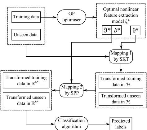
implementation of this module is based on the previous work of [15], because it supports a syntactically rich search space with sufficient expressive power to generate robust PP indices. Table 2 outlines the main steps of the GP-based search. Its main components, that is the chromosome encoding, the fitness function evaluation and the function and terminal sets are described in the following subsections. We refer to our proposed algorithm as evolutionary kernel sequential projection pursuit (EKSPP). Figure 1 presents an overview of the sequencing of the main operations supported by EKSPP, including model identification using training data and the final classification task using unseen data.
3.1 Chromosome Encoding
Each chromosome encodes three parts, that is a tree structure = representing the projection index, a real-valued array✓for the parameters of the adaptive kernel,
and an integer variable b for the dimensionality of the
extracted features. Thus, each ith member in the
[image:6.612.315.563.86.564.2]popu-lation of the GP module (see Table 2), is represented as the triplet ⇠i = [=i, bi,✓i]. This representation facilitates simultaneous evolution of both numeric and symbolic variables and, along with the function and terminal sets, it provides a highly expressive representation mecha-nism that enables the search to reach areas of the solution space that contain effective models.
TABLE 1
Description of the main steps for the computation of the classification errorE(⇠)of a given model⇠= [=, b,✓].
1) Input: Training setD, cross-validation partition sizek, tentative model parameters=,b, and✓.
2) Initialization:
a) PartitionDto kdifferent folds, each containing a subset
Difor training and its complementDi¯ for validation, for
i= 1, . . . , k.
b) Seti= 1.
3) Main loop: Whileikdo:
a) Compute dot-product matricesKw(i,✓)andK¯w(i,✓)with
Eqs. (13) and (29), respectively. b) SetK(1)
w (i,✓) =Kw(i,✓), andj= 0.
c) Whilejbdo:
i) Use constrained optimization to finde⇤j+1in Eq. (24).
ii) Update ⇤
j+1 using Eq. (23) (or set ⇤1 = e⇤1 when
j= 0).
iii) Update matrixK(j+1)
w using Eq. (25), and setj=j+ 1.
d) Compute the projected featuresZi=Kw(i,✓) ⇤b of
train-ing setDi, andZ¯i= ¯Kw(i,✓) ⇤
b of validation setDi¯.
e) Train the classifierCusingZiand their class label vector yi.
f) ApplyCon the validation featuresZ¯ito predict their labels ˆ
yi.
g) Estimate the classification errorEi=kyi¯ yikHˆ .
h) Seti=i+ 1.
4) OutputP : Return the overall validation error E([=, b,✓]) =
k i=1Ei.
Fig. 1. Overall description and flow of operations and data in the proposed system.
3.2 Fitness Evaluation
Given a specific model created either during population initialization or through an operator such as crossover or mutation, its fitness value has to be computed. The fitness evaluation of a given individual ⇠i = [=i, bi,✓i] first needs the calculation of the optimum projection coefficients ⇤
[image:6.612.319.556.357.567.2]TABLE 2
Description of the main GP operations of EKSPP. 1) Input: Set training setD, number of generationsGPgen,
popu-lation sizeGPpop.
2) Initialization:
a) Create random and hybrid individuals encoded by the chromosomes⇠i= [=i, bi,✓i], fori= 1, . . . , GPpop.
b) Compute the fitness valueE(⇠i)for each chromosome.
c) Sett= 1.
3) Main loop: WhiletGPgendo:
a) Select stochastically parents, and apply crossover and mu-tation to produce children⇠c
i, fori= 1, . . . , GPpop.
b) Compute the fitness valueE(⇠c
i)for each child, and insert
it into the population.
c) Keep the bestGPpopindividuals from the expanded
pop-ulation to be the new generation of individuals⇠i.
d) Sett=t+ 1.
4) Output: Locate the fittest individual⇠⇤in the population, and extract its corresponding parameters =, b, and ✓ to be the optimum model.
the coefficients are obtained with a constrained nonlinear optimization method. Any such method can be used in this step, because the index function and its parameters are known from the encoded chromosome. Here, we employ of a penalty function based on the objective
=(K(wj+1) )and the constraint TKw = 1, and optimize it with a standard Broyden-Fletcher-Goldfrab-Shanno (BFGS) method [40]. This is based on a quasi-Newton iterative update scheme (t+1) = (t) ↵tHt1rF( (t)). At each iteration t,↵tis an optimizing length along an optimum direction, rF(·) the gradient of the penalty function, and Ht a rank-two approximation of the Hes-sian matrix, so that an explicit computation is not needed.
3.3 Function and Terminal Sets
The function and terminal sets provide the building blocks to construct potential indices for the tree structure part of the chromosome. The expressive power achieved by rich function and terminal sets enables EKSPP to create not only most of the existing PP indices, such as PCA or ICA, but also new ones not considered before. The function set we use is summarized in Ta-ble 3. These functions are selected because of certain advantages. Basic arithmetic operands are very useful to combine more complex functions. The inclusion of R´enyi divergence, in conjunction with the generalized extreme value (GEV) and Student-t distributions, enables the GP module to potentially discover what can be considered as an interesting projection. R´enyi entropy is included as a generalization of the Shannon entropy, and together with R´enyi divergence provides a good approximation of the most popular unsupervised pro-jection indices. Furthermore, with suitable combinations of sample central moments, the evolutionary framework could potentially build any unsupervised moment-based index previously considered. Class means and variances, quartiles and within/between-scatters are included to build supervised indices.
TABLE 3
Proposed function set, wherez=Kw is the projection
of the training data with label vectory= [y1, . . . , yn]T that
associates each sampleziwith a class labelyifrom the
cavailable ones. Function Arity Description
+, -, *,
/, pow 2
Addition, subtraction, multiplication, divi-sion, and exponentiation
ms 2 sm-th sample central moment
s(z) =E[(z E(z))s]
D 5
R´enyi divergence
D(ˆf,g;⇢) = 1
⇢ 1log
d X
i=1
ˆ
fi⇢ gi⇢ 1
!
⇢>0,
whereg= [g1, . . . , gd]andˆf= [ ˆf1, . . . ,fˆd]
denotedbins of a reference pdfJ(t)and of the projected data pdf, respectively. It defines what could be considered as an uninteresting projection by means ofJ(t).
H 2
R´enyi entropy
H⇣ˆf;⇢⌘= 1 1 ⇢log
d X
i=1
ˆ
fi⇢ !
⇢ 0.
It has unique properties conferred by its
⇢coefficient, for example it can potentially deliver the Hartley entropy ofzwhen⇢= 0
and it converges to the Shannon entropy as
⇢!1.
Qji 4
Quartiles
They provide a robust alternative to get the dispersion and overall central tendency within each class, defined as
Qji⌘Q(i, j,y,z) =zl:l=|0.25·i·nj|,
whereQjirepresents theith quartile of class
j,nj is the number of projected samples
with class label j, andzl is thelth sample
in the ordered set.
µj 3 Class meansµ(j,y,z) =E[{z
i:yi=j}]
j 3 Class variances(j,y,z) =Ehn(z
i µj)2:yi=j oi
SW 2 Within-class scatterS
W(y,z) =Pcj=1 Pnj
i=1(zi µj)2
SB 2 Between-class scatterS
B(y,z) =Pcj=1(µj µ)2
The terminal set consists of the projected data z =
Kw , the class-vector y, and an ephemeral random constant ⌘ whose role is to provide a mechanism for
changing the values of several scalar parameters at the leaves of each potential projection index=. These scalar parameters are summarized in Table 4 and they are initialized to random values by different instances of ⌘
TABLE 4
Scalar terminal parameters (top) and GP parameters with their values (bottom).
Parameter description
Reference pdf selector⌧ for the R´enyi divergence.
Degrees of freedom%for the Student-t distribution. Shape parameter⇠for the GEV distribution. Coefficients⇢for the R´enyi entropy and divergence. Ordersof the momentms.
Quartile numberi.
Class indexjfor the class meanµj, class variance j,
andnth quartileQjn.
Maximum generationsGPgen=50 for the evolution.
Total population individualsGPpop= 20.
Crossover rateGPxover= 90%.
Mutation rateGPmut= 10%.
Tree depth for initializationGPtree= 8.
4 E
XPERIMENTATION ANDR
ESULTS 4.1 Experimental SetupSeven datasets (summarized in Table 5) are used to benchmark the proposed EKSPP. These include the arcene, dexter, dorothea and madelon datasets provided by the NIPS’03 challenge [41], also the duke data from [42], PIE data from the CMU PIE database as used in [43], and Reuters data from the “Reuters-21578 Text Catego-rization Test Collection” including samples possessing unique class labels. These datasets are chosen because of their high dimensionality. We compare EKSPP with two linear feature extraction methods including PCA and our previously proposed EPP [15], as well as the three popular nonlinear feature extraction methods of kernel PCA (KPCA), kernel LPP (KLPP) and kernel FDA (KFDA). The adaptive kernel in Eq. (2) is used for all competing kernel methods.
The four nonlinear methods of KPCA, KLPP, KFDA and EKSPP work in the non-observable space H in-duced by a kernel which equips them with a better capability for handling data nonlinearities compared to the linear methods of EPP and PCA. To further map the data from Hto a low-dimensional space Rb, KPCA attempts to highlight the global data statistics in the resulting space by maximizing the data variance along each data projection. KLPP attempts to preserve the local data geometry by minimizing the distances between closely related points defined based on the aggregate pairwise proximity information of the underlying lo-cal neighborhood graph. Both KPCA and KLPP are able to provide a compact representation of the data. However, as they work in an unsupervised manner that takes into account feature information only, the reduced features may not boost the final classification performance when there exists incompatibility between the original features and the class labels; for example, in many real-world classification applications, samples from different classes (or the same class) may be located closely (or distantly) in the feature space. To overcome this, the supervised method KFDA attempts to improve the separability between classes in the resulting space
TABLE 5
Cardinalities of the testing, training and validation datasets, number of features and classes, as well as median BER values for each set based on 10-fold CV.
Dataset information: Median BER values: Dataset Test Train Validation Features Classes l-SVM g-SVM MI+g-SVM arcene 20 120 60 10,000 2 27.94 23.94 12.26 dexter 60 360 180 20,000 2 18.46 13.46 17.70 dorothea 115 690 345 100,000 2 37.23 23.12 18.86 madelon 260 1560 780 500 2 41.10 24.87 51.23
duke 4 26 14 7129 2 12.26 8.33 19.0
PIE 1155 6933 3466 1024 68 51.03 43.12 46.37 Reuters 296 1775 891 2959 11 20.37 13.27 23.30
by arranging samples from the same class proximaly, while those from different classes apart. Nevertheless, this may distort the intrinsic geometry of the original space and lead to an overfitted situation of the labeled samples. Differently, the proposed EKSPP combines both advantages of KFDA (utilization of label information) and KPCA/KLPP (avoidance of overfitting) by evolving an optimal PP index from a very diverse function pool designed to characterize both the feature-driven data statistics and geometry as well as the label-driven class scatters (see Table 3). In the following experiments, we compare these methods to examine how they contribute to different classification tasks.
We employ 10-fold cross validation (CV) to evaluate the classification performance. For each partition, the dataset is split into two mutually exclusive sets. The training set is used for complete model selection using Eqs. (32), (33) (with k = 3, to further partition it to
training and validation). Once the optimal model is determined, the other set is used to test its generalization ability based on the accumulated balanced error rate (BER). This is the average of the false positive rates of difference classes computed as
BER⌘1
c
c
X
i=1
FPi
ni
, (34)
where FPi and ni denote the number of false positives and the class size, respectively, for the ith class. This procedure is repeated ten times in total, and the medi-ans and interquartile ranges (IQR) of the recorded BER values are reported as the final classification results.
4.2 Implementation of the Evolutionary Optimization
Since both EKSPP and EPP methods rely on symbolically selecting the PP index=, they require GP-assisted opti-mization. We implement this using the GPLAB library [44], and the parameters and values shown in Table 4. The genetic operators handle the different parts of each chromosome independently. Whenever crossover is se-lected during the reproduction stage, standard one-point crossover is applied to the tree part of the chromosome that encodes the index=, while arithmetic crossover is applied to each component of the numerical part that encodes b and ✓ = [✓1,✓2,✓3]. The mutation operator
TABLE 6
Comparison of the median and IQR of BER over a 10-fold CV for different feature extraction algorithms. The best performance within each dataset is underlined.
arcene dexter dorothea madelon duke PIE Reuters
Method Median IQR Median IQR Median IQR Median IQR Median IQR Median IQR Median IQR PCA 25.83 18.66 35.26 5.62 41.19 4.63 43.13 5.62 7.21 3.21 40.54 8.23 17.57 8.52 EPP 16.67 12.49 32.18 3.47 18.27 7.10 29.57 3.47 7.01 4.72 36.44 2.72 12.24 3.31 KPCA 23.14 28.28 33.15 11.25 27.42 7.14 31.21 6.56 6.98 6.10 35.82 7.14 10.11 2.03 KLPP 20.44 6.52 19.94 7.08 17.10 11.36 24.83 3.11 9.63 6.98 53.81 10.26 45.66 2.31 KFDA 16.38 19.49 18.86 22.48 20.08 5.37 24.74 1.12 4.87 3.83 27.85 12.47 23.69 7.09 EKSPP 10.10 4.32 11.40 5.83 11.92 8.36 23.20 4.92 5.43 2.71 27.17 7.06 9.75 0.85
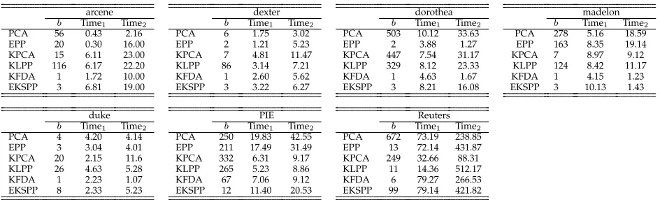
TABLE 7
Comparison of the reduced feature dimensionalityb, and computational times for the model selection (Time1, in
hours) and for the out-of-sample projection (Time2, in seconds), for the different algorithms.
arcene dexter dorothea madelon
b Time1 Time2 b Time1 Time2 b Time1 Time2 b Time1 Time2
PCA 56 0.43 2.16 PCA 6 1.75 3.02 PCA 503 10.12 33.63 PCA 278 5.16 18.59 EPP 20 0.30 16.00 EPP 2 1.21 5.23 EPP 2 3.88 1.27 EPP 163 8.35 19.14 KPCA 15 6.11 23.00 KPCA 7 4.81 11.47 KPCA 447 7.54 31.17 KPCA 7 8.97 9.12 KLPP 116 6.17 22.20 KLPP 86 3.14 7.21 KLPP 329 8.12 23.33 KLPP 124 8.42 11.17 KFDA 1 1.72 10.00 KFDA 1 2.60 5.62 KFDA 1 4.63 1.67 KFDA 1 4.15 1.23 EKSPP 3 6.81 19.00 EKSPP 3 3.22 6.27 EKSPP 3 8.21 16.08 EKSPP 3 10.13 1.43
duke PIE Reuters
b Time1 Time2 b Time1 Time2 b Time1 Time2
PCA 4 4.20 4.14 PCA 250 19.83 42.55 PCA 672 73.19 238.85 EPP 3 3.04 4.01 EPP 211 17.49 31.49 EPP 13 72.14 431.87 KPCA 20 2.15 11.6 KPCA 332 6.31 9.17 KPCA 249 32.66 88.31 KLPP 26 4.63 5.28 KLPP 265 5.23 8.86 KLPP 11 14.36 512.17 KFDA 1 2.23 1.07 KFDA 67 7.06 9.12 KFDA 6 79.27 266.53 EKSPP 8 2.33 5.23 EKSPP 12 11.40 20.53 EKSPP 99 79.14 421.82
a node and substitutes its branch with a newly created random subtree. For the numerical parts, it replaces their current values with alternative ones, randomly taken from valid ranges depending on the variable be-ing mutated. The initial population is generated with the ramped half-and-half method. To select parent sets for mating, we used lexicographic parsimony pressure tournament as the sampling technique, in order to favor short trees over competing individuals when fitnesses were equal. Encouraging parsimony promotes simpler indices which are easy to interpret. Finally, in order to accelerate search and afford smaller populations, we also hybridize the population with some well known sim-ple models that may perform well for some problems. Specifically, two of the members of the initial population are initialized to be those of KFDA and KPCA, while the remaining are randomly created as stated above.
The three nonlinear algorithms of KPCA, KLPP and KFDA require the tuning of a set of model parameters, such as b and ✓. We optimize these parameters using a
genetic algorithm (GA). It should be noted, that a GP is not needed in this case, as the methods KPCA, KLPP and KFDA do not have a PP index to evolve symbolically, but their indices are instead fixed as implied by their original designs. Because EKSPP, in addition to b and ✓, also
needs the symbolic estimation of an index = that best suits the given data, its model training is implemented with the previously described GP module. Nevertheless, in order to maintain an objective experimental compar-ison, the GA for KPCA, KLPP and KFDA has identical
setup and parameters with the part of the GP for EKSPP that optimizes the numerical chromosome components (that is the crossover, mutation and reproduction opera-tors, excluding the operations for the symbolic tree part of the chromosome).
4.3 Comparative Analysis
To investigate the potential separability of the employed datasets in advance, we perform a preliminary study using a linear support vector machine (SVM) (l-SVM), a nonlinear SVM with Gaussian kernel (g-SVM), as well as the combination of g-SVM and a sequential forward feature selection based on mutual information (MI+g -SVM). Their classification performance (median BER) is recorded in Table 5 along with the datasets information. From the last three columns of Table 5, it can be observed that g-SVM always performs better than l-SVM. This indicates that the used datasets possess nonlinear struc-tures with classes that cannot be well separated with linear boundaries. Also, MI+g-SVM does not provide better performance thang-SVM for most datasets, which indicates that the classification task does not always benefit from simple feature selection.
[image:9.612.71.543.218.361.2]features in the lower dimensional space, especially those obtained by EKSPP, possess much better class separa-bilities than the original features or subsets of them. This demonstrates the effectiveness of dimensionality reduction via feature extraction. Next, examining Table 6 where performance ranking for the competing methods differs across the datasets, indicates that none of them can claim superiority over the rest, while the proposed EKSPP performs the best for almost all the datasets. This is because EKSPP sustains a data-driven adapta-tion of the feature extracadapta-tion process, which recovers the kernel parameters and the symbolic form of the PP index most suitable to the data and the current classification task. Specifically, between a pair of linear and nonlinear versions of an algorithm, e.g., PCA vs. KPCA, or EPP vs. EKSPP, the nonlinear version leads to a performance improvement between 2%to 20%for most datasets. This is because linear projections cannot handle data nonlinearities when they exist, whereas nonlinear projections can handle diverse linear or nonlinear data characteristics as controlled by the adaptive kernel.
Among the four nonlinear algorithms of KPCA, KLPP, KFDA and EKSPP, the unsupervised KPCA and KLPP are in general weaker than the supervised KFDA and EKSPP. However, for the dorothea and Reuters datasets, performance of the supervised method KFDA (around 20%and 24%in BER) is actually worse than the unsuper-vised performance (around 17% and 10% in BER). This experimentally supports what we discussed in Section 4.1, that is considering only the label-driven class scatters but ignoring the feature-driven data statistics may not lead to good generalization for some datasets. Although the nonlinear and supervised KFDA is quite competitive for several datasets, the proposed EKSPP performs sig-nificantly better with between 6%and 14%improvement for four out of the seven datasets, and slightly bet-ter or comparable performance for the remaining three datasets. For example, the BER of dorothea and Reuters datasets, for which KFDA possesses poorer performance than the unsupervised methods, has been improved to less than 12%and 10%. This shows that by evolving an optimal PP index which takes into account both feature and class information, EKSPP is able to offer better classification control than KFDA when overfitting may occur.
Table 7 records the reduced dimensionalities as well as the computational times of the model selection phase and the out-of-sample projection for the proposed and competing methods across different datasets. By com-paring the reduced dimensionalities, it can be seen that for most datasets EKSPP is capable of generating a small set of features with satisfactory class separability from the original high-dimensional feature space. For the binary classification case, EKSPP can never be of course better than KFDA in terms of its reduction rate, since KFDA is designed to generate only c 1 = 1 feature, while for the multi-class classification case it generates no more than c 1features. However, drastic
dimensionality reduction often occurs at the expense of classification performance. For example, among the six datasets where KFDA extracts the least number of fea-tures, four datasets possess poor KFDA performance (6% and 14%worse than EKSPP). It should also be noted, that for many real-world applications, e.g., text categorisation and computer-aided diagnosis, as long as a reasonably small set of features is extracted, it is not necessary to further suppress the feature dimensionality to less than the number of classesc. Moreover, if the imposition of an
upper bound on the resulting dimensionality is critical for a given application, EKSPP can support this through the explicit incorporation of this bound by restricting the search range ofb.
By comparing the computational times, it can be seen that, although the model selection stage of EKSPP is not the fastest compared to the competing ones, this is because the method has the most complex model, as it additionally searches for the best PP index formula and the best kernel parameters that optimally suit the classification task. Overall, between the two supervised methods of EKSPP and KFDA, although KFDA may lead to better compression for certain cases and requires less training time, it does not provide as good performance as EKSPP. EKSPP is suitable for processing challenging datasets where traditional feature methods based on fixed model, e.g, KFDA, is not sufficient, and additional effort for more suitable feature representation formulae is necessitated.
All the experiments reported here are based on the GP parameters of Table 4 discussed in Section 4.2. These control the balance between finding good solutions and doing so within reasonable processing times, something directly related to the number of objective function evaluations. As seen from Table 2, the number of func-tion evaluafunc-tions depends on the parametersGPgen and
GPpop. To examine the sensitivity and robustness of the
proposed optimization, we experimented with different settings for GPgen and GPpop. We found that although larger values increase significantly the running times, they did not show notable BER improvement (less than 5%). The currently used small number of GPpop = 20 members evolved for few GPgen = 50 generations are adequate. This is because of the expressive function set of Table 3 capable of readily capturing representa-tive feature characteristics and label related information. Moreover, the use of hybridization helps to start up the population with some competent initial solutions which have the potential to rapidly influence subsequent generations. Another issue regarding the current param-eter setting, is the complementary values of GPxover and GPmut that control the fraction of Gpop offspring generated via crossover or mutation. These can affect the balance between exploiting building blocks currently in the population and exploring new regions of the solution space. Experimentations showed that as long as
10 15 20 25 30 35 40 6
8 10 12 14 16 18 20 22
(a) Original, SD1
5 10 15 20 25 30
5 10 15 20 25 30
(b) Original, SD2
5 10 15 20 25 30
5 10 15 20 25 30
(c) Original, SD3
−1 −0.5 0 0.5 1 1.5 2 −2
−1.5 −1 −0.5 0 0.5 1 1.5 2
(d) EPP, SD1
−1.5 −1 −0.5 0 0.5 1 1.5 2
−2
−1.5
−1
−0.5 0 0.5 1 1.5 2
(e) EPP, SD2
−1.5 −1 −0.5 0 0.5 1 1.5
−2
−1.5
−1
−0.5 0 0.5 1 1.5 2
(f) EPP, SD3
−0.05 0 0.05 0.1
−0.04 −0.02 0 0.02 0.04 0.06 0.08
(g) EKSPP, SD1
−0.12−0.1−0.08−0.06−0.04−0.02 0 0.020.040.060.08
−0.1
−0.05 0 0.05 0.1
(h) EKSPP, SD2
−0.1 −0.05 0 0.05 0.1 0.15
−0.3
−0.25
−0.2
−0.15
−0.1
−0.05 0 0.05 0.1
(i) EKSPP, SD3
Fig. 2. Comparison between the original features of three synthetic datasets SD1, SD2 and SD3, and the corresponding features extracted by EPP and EKSPP. Different patterns/shades indicate different data classes.
1 1.5 2 2.5 3 3.5 4 4.5 5 0
500 1000 1500 2000 2500
log10m
CPU time in seconds
original kernel
Fig. 3. Comparison of the whitening procedure CPU times in the original and kernel-induced spaces, using the dorothea dataset and increasing number of features.
over the late generations stagnates as the search cannot explore effectively new regions of the solution space. Conversely, a rate over 30% makes mutation somewhat too disruptive and requires many more generations to produce a good model.
Since a primary contribution of this work is to en-able the evolutionary PP engine to operate in a kernel-induced space, we additionally demonstrate two advan-tages with regard to the use of kernels. These are the capability for handling nonlinear structures within com-plex data and that of improving the computational effi-ciency when processing large-scale features. To demon-strate the former, we compare the two evolutionary engines of EPP [15] and the proposed EKSPP using three two-dimensional datasets possessing nonlinear shapes.
These include a classical compound dataset [45], referred to as SD1, and two path-based synthetic datasets [46], referred to as SD2 and SD3. The distributions of the original features and those of the extracted features by EPP and EKSPP are plotted in Figure 2. Comparing the original feature distributions in Figures 2(a), 2(b) and 2(c) with their corresponding EPP generated ones in Figures 2(d), 2(e) and 2(f), it can be seen that EPP does not provide any major changes to the data apart from simple scaling and rotation. This is expected as EPP applies only linear projections to the original feature space. The results of EKSPP in Figures 2(g), 2(h) and 2(i), however, show that the nonlinearities of the data have been unfolded successfully. This is because linear projections in the kernel-induced feature space are equiv-alent to nonlinear feature transformations in the original space. The supported computational efficiency can be demonstrated with the aid of the whitening procedure. As explained in Section 2.2, whitening requires the de-composition of a data matrix withmcolumns (wherem
is equal to the number of original features), whereas in the kernel-induced space it requires the decomposition of an n⇥n kernel matrix (where n is the number of
training samples). The incurred computational cost for the former case is aroundO(m3)orO(mn2)depending
on whether eigen-decomposition or singular value de-composition is used for the PCA, while for the latter case it is of O(n3) [47]. Therefore, whitening is very
computationally sensitive to an increased number of features when applied in the original feature space than in the kernel-induced space. In Figure 3, we compare the CPU times for whitening with and without kernels, based on 800 data samples from the dorothea dataset and for increasing dimensionalities, running Matlab 7.1 on a 3.4-GHz CPU machine with 16-GB memory under Mac OS X.8. It can be seen that for low number of features, such as m <103, the computational costs of both cases
are comparable. However, as dimensions increase, such as when m > 104, the use of kernels greatly reduces
the cost by converting the decomposition of a covariance matrix to that of a kernel matrix.
5 CONCLUSION
[image:11.612.53.298.52.278.2] [image:11.612.76.272.351.499.2]R
EFERENCES[1] I. T. Jolliffe, Principal Component Analysis. New York, USA: Springer-Verlag, 2002.
[2] A. Hyvarinen, J. Karhunen, and E. Oja, Independent Component Analysis. New York, USA: Wiley, 2001.
[3] S. Theodoridis and K. Koutroumbas,Pattern Recognition, 2nd ed. New York, USA: Academic, 2003.
[4] X. He and P. Niyogi, “Locality preserving projections,” inProc. of Neural Information Processing Systems 16, NIPS, 2003.
[5] B. Sch¨olkopf, A. Smola, and K. R. M ¨uller, “Nonlinear component analysis as a kernel eigenvalue problem,” Neural Computation, vol. 10, no. 5, pp. 1299–1319, 1998.
[6] B. Sch¨olkopf, S. Mika, C. J. C. Burges, P. Knirsch, K.-R. M ¨uller, G. R¨atsch, and A. J. Smola, “Input space versus feature space in kernel-based methods,”IEEE Trans. Neural Network, vol. 10, no. 5, pp. 1000–1017, 1999.
[7] E. Pekalska, P. Paclik, and R. P. W. Duin, “A generalized kernel approach to dissimilarity-based classification,”Journal of Machine Learning Research, vol. 2, pp. 175–211, 2002.
[8] T. Mu, M. Makoto, J. Tsujii, and S. Ananiadou, “Discovering robust embeddings in (dis)similarity space for high-dimensional linguistic features,”Computational Intelligence, 2013, in press. [9] T. Mu, J. Y. Goulermas, J. Tsujii, and S. Ananiadou,
“Proximity-based frameworks for generating embeddings from multi-output data,” IEEE Trans. on Pattern Analysis and Machine Intelligence, vol. 34, no. 11, pp. 2216–2232, 2012.
[10] T. Mu, J. Jiang, Y. Wang, and J. Y. Goulermas, “Adaptive data embedding framework for multi-class classification,”IEEE Trans. on Neural Networks and Learning Systems, vol. 23, no. 8, pp. 1291– 1303, 2012.
[11] C. Yang, L. Wang, and J. Feng, “On feature extraction via kernels,”
IEEE Trans. Systems, Man, and Cybernetics, Part B: Cybernetics, vol. 38, no. 2, pp. 553–557, 2008.
[12] L. Sun, S. Ji, and J. Ye, “Hypergraph spectral learning for multi-label classification,” inProc. of the 14th ACM SIGKDD International Conference on Knowledge Discovery and Data Mining, Las Vegas, Nevada, USA, 2008, pp. 668–676.
[13] S. Yan, D. Xu, B. Zhang, H.-J. Zhang, Q. Yang, and S. Lin, “Graph embedding and extensions: A general framework for di-mensionality reduction,”IEEE Trans. Pattern Analysis and Machine Intelligence, vol. 29, no. 1, pp. 40 –51, 2007.
[14] H. Li, T. Jiang, and K. Zhang, “Efficient and robust feature extraction by maximum margin criterion,”IEEE Trans. on Neural Network, vol. 17, no. 1, pp. 157–165, 2006.
[15] E. Rodriguez-Martinez, J. Goulermas, T. Mu, and J. Ralph, “Auto-matic induction of projection pursuit indices,”IEEE Trans. Neural Networks, vol. 21, no. 8, pp. 1281 –1295, August 2010.
[16] M. Jones and R. Sibson, “What is projection pursuit?”Journal of the Royal Statistical Society, vol. 150, no. 1, pp. 1–37, 1987. [17] H. Friedman and J. Tukey, “A projection pursuit algorithm for
exploratory data analysis,” IEEE Trans. Computers, vol. 23, pp. 881–889, 1974.
[18] Q. Guo, W. Wu, D. Massart, C. Boucon, and S. de Jong, “Sequen-tial projection pursuit using genetic algorithms for data mining of analytical data,”Analytical Chemistry, vol. 72, no. 13, pp. 2846– 2855, 2000.
[19] S.-S. Chiang, C.-I. Chang, and I. Ginsberg, “Unsupervised target detection in hyperspectral images using projection pursuit,”IEEE Trans. Geoscience and Remote Sensing, vol. 39, no. 7, pp. 1380–1391, Jul 2001.
[20] C.-T. Chu, J.-N. Hwang, H.-I. Pai, and K.-M. Lan, “Tracking human under occlusion based on adaptive multiple kernels with projected gradients,”IEEE Trans. on Multimedia, vol. 15, no. 7, pp. 1602–1615, Nov 2013.
[21] T. Dieth and M. Girolami, “Online learning with (multiple) ker-nels,”Neural Computation, vol. 25, no. 3, pp. 567–625, 2013. [22] J. Huang, X. You, Y. Yuan, F. Yang, and L. Lin, “Rotation invariant
iris feature extraction using gaussian markov random fields with non-separable wavelet,” Neurocomputing, vol. 73, pp. 883–894, 2010.
[23] C. Coello, Evolutionary algorithms for solving multi-objective prob-lems. Boston, MA: Springer, 2007.
[24] Y.-T. Wu and F. Y. Shih, “Genetic algorithm based methodology for breaking the steganalytic systems,”IEEE Trans. Systems, Man, and Cybernetics, Part B: Cybernetics, vol. 36, no. 1, pp. 24–31, 2006.
[25] J. Liu, W. Zhong, and L. Jiao, “A multiagent evolutionary algo-rithm for constraint satisfaction problems,”IEEE Trans. Systems, Man, and Cybernetics, Part B: Cybernetics, vol. 36, no. 1, pp. 54–73, feb 2006.
[26] I. Ciornei and E. Kyriakides, “Hybrid ant colony-genetic algo-rithm (gaapi) for global continuous optimization,” IEEE Trans. Systems, Man, and Cybernetics, Part B: Cybernetics, vol. 42, no. 1, pp. 234–245, 2012.
[27] K. Xing, L. Han, M. Zhou, and F. Wang, “Deadlock-free ge-netic scheduling algorithm for automated manufacturing systems based on deadlock control policy,”IEEE Trans. Systems, Man, and Cybernetics, Part B: Cybernetics, vol. 42, no. 3, pp. 603–615, 2012. [28] S. Mabu, K. Hirasawa, O. Kotaro, and et al, “Enhanced decision
making mechanism of rule-based genetic network programming for creating stok trading signals,”Expert Systems with Applications, vol. 40, no. 6, 2012.
[29] M. Pedergnana, P. R. Marpu, M. D. Mura, J. A. Benediktsson, and L. Bruzzone, “A novel technique for optimal feature selection in attribute profiles based on genetic algorithms,” IEEE Trans. Geoscience and Remote Sensing, vol. 52, no. 6-2, 2013.
[30] P. Palmes, T. Hayasaka, and S. Usui, “Mutation-based genetic neural network,”IEEE Trans. Neural Networks, vol. 16, no. 3, pp. 587–600, May 2005.
[31] W.-S. Zheng, J.-H. Lai, and P. Yuen, “Ga-fisher: a new lda-based face recognition algorithm with selection of principal compo-nents,”IEEE Trans. Systems, Man, and Cybernetics, Part B: Cyber-netics, vol. 35, no. 5, pp. 1065 –1078, oct. 2005.
[32] J. L. Olmo, J. R. Romero, and S. Ventura, “Using ant programming guided by grammar for building rule-based classifiers,” IEEE Trans. Systems, Man, and Cybernetics, Part B: Cybernetics, vol. 41, no. 6, 2011.
[33] W. L. Tung and C. Quek, “eFSM - a novel online neural-fuzzy semantic memory model,” IEEE Trans. Neural Networks, vol. 21, no. 1, pp. 136–157, 2010.
[34] W.-C. Yeh, “New parameter-free simplified swarm optimization for artificial neural network training and its application in the pre-diction of time series,”IEEE Trans. Neural Networks and Learning Systems, vol. 24, no. 4, pp. 661–665, 2013.
[35] D. Muni, N. Pal, and J. Das, “Genetic programming for simulta-neous feature selection and classifier design,”IEEE Trans. Systems, Man, and Cybernetics, Part B, vol. 36, no. 1, pp. 106–117, 2006. [36] M. W. Aslam, Z. Zhu, and A. K. Nandi, “Feature generation
us-ing genetic programmus-ing with comparative partner selection for diabetes classification,”Expert Systems with Applications, vol. 40, no. 13, 2013.
[37] ——, “Automatic modulation classification using combination of genetic programming and knn,”IEEE Trans. Wireless Communica-tions, vol. 11, no. 8, pp. 2742–2750, 2010.
[38] Y. Zhang and P. I. Rockett, “A generic optimising feature extrac-tion method using multiobjective genetic programming,”Applied Soft Computing, vol. 11, no. 1, pp. 1087–1097, 2011.
[39] P. G. Espejo, S. Ventura, and F. Herrera, “A survey on the application of genetic programming to classification,”IEEE Trans. Systems, Man, and Cybernetics, Part C: Applications and Reviews, vol. 40, no. 2, 2012.
[40] J. Nocedal and S. J. Wright, Numerical Optimization, 2nd ed. Springer, 2006.
[41] “NIPS’03 feature selection challenge, december 8-13,” 2003. [Online]. Available: http://www.nipsfsc.ecs.soton.ac.uk
[42] M. West, C. Blanchette, H. Dressman, E. Huang, S. Ishida, R. Spang, H. Zuzan, J. A. Olson, J. R. Marks, and J. R. Nevins, “Predicting the clinical status of human breast cancer by using gene expression profiles,” in Proc. National Academy of Sciences, vol. 98, 2001, pp. 11 462–11 467.
[43] X. He, S. Yan, Y. Hu, P. Niyogi, and H.-J. Zhang, “Face recognition using laplacianfaces,” IEEE Trans. Pattern Analysis and Machine Intelligence, vol. 27, no. 3, pp. 328 –340, 2005.
[44] S. Silva and J. Almeida, “GPLABf: A genetic programming tool-box,” inProc. Nordic MATLAB Conference, 2003, pp. 273–278. [45] C. T. Zahn, “Graph theoretical methods for detecting and
describ-ing gestalt clusters,”IEEE Trans. Computers, vol. 100, no. 1, pp. 68–86, 1971.
[46] H. Chang and D. Y. Yeung, “Robust path-based spectral cluster-ing,”Pattern Recognition, vol. 41, no. 1, pp. 191–203, 2008. [47] T. Mu, M. Makoto, J. Tsujii, and S. Ananiadou, “Discovering
Eduardo Rodriguez-Martinez received the M.Sc. degree in information and intelligence en-gineering and the Ph.D. from the University of Liverpool, Liverpool, U.K., in 2008 and 2012, respectively. He is currently with the Department of Electrical Engineering and Electronics, at Uni-versidad Autonoma Metropolitana, Mexico City, Mexico. His current research interests include the fields of evolutionary computation, feature extraction, pattern recognition, and robotics.
Tingting Mu(M’05) (M’05) received the B.Eng. degree in electronic engineering and informa-tion science from the University of Science and Technology of China, Hefei, China, in 2004, and the Ph.D. degree in electrical engineering and electronics from the University of Liverpool, U.K., in 2008. She is currently a Lecturer in the School of Electrical Engineering, Electronics and Com-puter Science at the University of Liverpool, U.K. Her current research interests include machine learning, data analysis and mathematical mod-elling, with applications to information retrieval, text mining and bioinfor-matics.