On improving the selection of Thellier-type paleointensity data

(1)

RESEARCH ARTICLE

10.1002/2013GC005135

On improving the selection of Thellier-type paleointensity data

Greig A. Paterson1_{, Lisa Tauxe}2_{, Andrew J. Biggin}3_{, Ron Shaar}2_{, and Lori C. Jonestrask}2

1_{Key Laboratory of Earth’s Deep Interior, Institute of Geology and Geophysics, Chinese Academy of Sciences, Beijing,}

China,2Geosciences Research Division, Scripps Institution of Oceanography, University of California San Diego, La Jolla,

California, USA,3_{Geomagnetism Laboratory, Department of Geology and Geophysics, School of Environmental Sciences,}

University of Liverpool, Oliver Lodge Laboratories, Liverpool, UK

Abstract

The selection of paleointensity data is a challenging, but essential step for establishing data reliability. There is, however, no consensus as to how best to quantify paleointensity data and which data selection processes are most effective. To address these issues, we begin to lay the foundations for a more unified and theoretically justified approach to the selection of paleointensity data. We present a new compi-lation of standard definitions for paleointensity statistics to help remove ambiguities in their calcucompi-lation. We also compile the largest-to-date data set of raw paleointensity data from historical locations and laboratory control experiments with which to test the effectiveness of commonly used sets of selection criteria. Although most currently used criteria are capable of increasing the proportion of accurate results accepted, criteria that are better at excluding inaccurate results tend to perform poorly at including accurate results and vice versa. In the extreme case, one widely used set of criteria, which is used by default in the Thellier-Tool software (v4.22), excludes so many accurate results that it is often statistically indistinguishable from randomly selecting data. We demonstrate that, when modified according to recent single domain paleoin-tensity predictions, criteria sets that are no better than a random selector can produce statistically signifi-cant increases in the acceptance of accurate results and represent effective selection criteria. The use of such theoretically derived modifications places the selection of paleointensity data on a more justifiable theoretical foundation and we encourage the use of the modified criteria over their original forms.

1. Introduction

Reconstructing the evolution of Earth’s geodynamo requires detailed and accurate records of long-term geomagnetic field variations. Obtaining reliable estimates of the ancient geomagnetic field strength (paleo-intensity) can be a challenge and numerous factors, such as chemical alteration or multidomain (MD) grains, result in high data rejection rates, or the acceptance of inaccurate results. The use of appropriate selection criteria to discriminate against such factors is essential if we want to understand long-term paleointensity behavior. At present paleointensity data selection is a notoriously arbitrary process that lacks a solid theoret-ical foundation. The modern approach to data selection was established 35 years ago byCoe et al. [1978], but despite numerous investigations of paleointensity statistics [e.g.,Tauxe and Staudigel, 2004;Chauvin et al., 2005;Biggin et al., 2007;Paterson et al., 2012], no consensus exists as to how to select paleointensity data appropriately. In this study, we lay the foundations for an approach to paleointensity data selection that removes ambiguity and transforms the selection process into a more theoretically justifiable endeavor.

To date, more than 40 paleointensity statistics have been proposed and are used regularly in modern stud-ies. Differences in the details of the calculations between different laboratories or software packages often mean that data, and statistical characterization thereof, are inconsistent. To overcome this, we introduce the Standardized Paleointensity Definitions (section 2), which is a new reference document that outlines the definitions and calculations of paleointensity data. In section 3, we describe the largest-to-date compilation of raw paleointensity data from experiments where the true paleointensity is known. This is now available for download from the MagIC database (earthref.org/MAGIC/). In this section, we also outline current data selection criteria sets and new analyses to quantify and assess their effectiveness. Using these analyses and the compiled data set, we assess the effectiveness of commonly used sets of selection criteria in section 4. We then modify these criteria sets according to theoretically predicted ideal single domain (SD) behavior [Paterson et al., 2012;Paterson, 2013] and demonstrate that these modifications improve the overall success of the selection process.

Special Section:

Magnetism From Atomic to Planetary Scales: Physical Principles and Interdisciplinary Applications in Geo- and Planetary Sciences

Key Points:

Standard deﬁnitions for

paleointensity statistics are proposed A large paleointensity meta-analysis

is conducted to investigate data selection

Modiﬁcations based on SD predictions improve the effectiveness of selection

Supporting Information:

SPD v1.0 ReadMe

Correspondence to:

G. A. Paterson,

[email protected]

Citation:

Paterson, G. A., L. Tauxe, A. J. Biggin, R. Shaar, and L. C. Jonestrask (2014), On improving the selection of Thellier-type paleointensity data,Geochem. Geophys. Geosyst.,15, 1180–1192, doi:10.1002/2013GC005135.

Received 6 NOV 2013 Accepted 1 MAR 2014

Accepted article online 5 MAR 2014 Published online 22 APR 2014

Geochemistry, Geophysics, Geosystems

(2)

2. Standardizing Paleointensity Statistics

Through the authors’ experiences, discussions with the paleomagnetic community, examination of open source code, and through reanalysis of published data, it has become clear that there are inconsistencies in the quantification of paleointensity statistics. Many of these inconsistencies are small and may be attributed to numerical rounding. Others, however, are more substantial and may influence the outcome of data selec-tion and the comparison of studies. One example is the fracselec-tion (f) of natural remanent magnetization (NRM) used for the best-fit on the Arai plot [as defined byCoe et al., 1978], which is one of the most widely used paleointensity statistics. Through our work, we have encountered three different methods of calculat-ingf, which can be substantially different.

To ensure that paleointensity statistics are consistently calculated we have written the Standard Paleointen-sity Deﬁnitions (SPD). SPD outlines both the textual and mathematical deﬁnitions for the calculation of pale-ointensity estimates and for over 40 statistics used to select data. SPD also describes the theory and mathematics of applying corrections to paleointensity data affected by anisotropic thermoremanent mag-netization (TRM) [Veitch et al., 1984;Chauvin et al., 2000] and nonlinear TRM acquisition [Selkin et al., 2007].

The SPD is a reference document to allow paleointensity analysts to consistently quantify their data. To facili-tate this, the SPD includes numerical and programming advice that will help to ensure that paleointensity data are accurately and efﬁciently determined across all platforms of analysis. In addition, we provide a refer-ence data set, which contains the raw paleointensity data and the statistics for 20 specimens. This data set can be used by developers of paleointensity software to ensure that their analyses are consistent with SPD.

Version 1.0 of the SPD is attached as supporting information. This and future versions of SPD along with examples code are available from http://www.paleomag.net/SPD. We welcome all comments and sugges-tions to help further improve SPD and the consistency of paleointensity analysis.

3. Data and Methods

3.1. Historical Data

To investigate the effectiveness of paleointensity data selection, we require an extensive data set from mens where the expected paleointensity is known. To that end, we have compiled the raw data from 395 speci-mens obtained from historical volcanoes or laboratory experiments. The data set is summarized in Table 1 and consists of data from 13 studies, which represent 15 localities or laboratory experiments (18 unique heating events). Full details of the experimental protocols and measurements are given in the respective references.

All studies used variants of the Coe or IZZI protocols [Coe, 1967;Yu et al., 2004] using either conventional thermal [e.g.,Yamamoto and Hoshi, 2008] or microwave techniques [Biggin et al., 2007]. Thirty-six specimens (9%) are from the microwave technique [Biggin et al., 2007] and 54 (14%) from the IZZI protocol [ Pater-son et al., 2010b;Shaar et al., 2010]. The largest data set from a single event is that ofBowles et al. [2006], which contains 53 specimens and constitutes13% of the data set. Our compilation is composed of a range of different materials and includes geological as well as archeological materials. Basalts and andesites are the most abundant material in the data set contributing 128 (33%) and 117 (30%) specimens, respectively. Synthetic magnetite specimens, which are typically MD in nature [Muxworthy, 1998;Krasa et al., 2003], constitute<3% of the entire data set. The diversity of the data set means that our results should not be systematically biased by data from any single study.

The availability of the original raw data allows the calculation of paleointensity statistics that were not used in the original studies. All statistics are calculated according to SPD v1.0. Where required, anisotropy and nonlinear TRM corrections have been made, but cooling rate corrections are not necessary or are negligible (10%) for these specimens, due to either grain size considerations [Biggin et al., 2013] or given that NRM and laboratory TRM cooling rates are known to be identical. To allow comparison between different studies, paleointensity estimates are normalized by the expected values. All of the data are available for download from the MagIC database or from http://www.paleomag.net/SPD.

3.2. Paleointensity Selection Criteria

(3)

2004], SELCRIT2 [Biggin et al., 2007], and the ThellierTool A and B criteria sets [Leonhardt et al., 2004] (herein referred to as TTA and TTB, respectively). The deﬁnitions of the statistics used in these sets are given in the SPD and the threshold values used for selection are given in Table 2. The TTA and TTB criteria are the default values from v4.22 of the ThellierTool. We note that PICRIT03 uses the criteriona0₁₅_{, where}_a0_{is the angular} difference between the anchored best ﬁt direction from the paleointensity experiment and an independent measure of the paleomagnetic direction (e.g., from a separate demagnetization experiment or a known direc-tion). Only about half of the specimens are oriented such as to allow a comparison with an expected direction. We therefore apply PICRIT03 without thea0₁₅_{criterion. Not all of the data include partial TRM (pTRM) or} pTRM tail checks; however, in these cases only four specimens do not have pTRM checks and 65 (16%) do not have tail checks. In these minority cases, absence of a check is regarded as failing to pass the check crite-ria, but the excluded data contribute to the assessment of the effectiveness of selection.

[image:3.630.47.585.115.343.2]

Recently,Paterson et al. [2012] developed a stochastic paleointensity model of ideal SD specimens that experience expected levels of experimental noise. They used this model to investigate the behavior of the

Table 2.The Sets of Selection Criteria Investigateda

Criterion PICRIT03

PICRIT03

(Modified) SELCRIT2

SELCRIT2

(Modified) TTA

TTA

(Modified) TTB

TTB (Modified)

n 4 4 4 4 5 5 5 5

f 0.35 0.35 0.15 0.35 0.5 0.35 0.3 0.35

b 0.1 0.1 0.1 0.1 0.1 0.1 0.15 0.15

q 2 2 1 1 5 5 0 0

MADAnc 7 7 15 15 6 6 15 15

a – – 15 15 15 15 15 15

npTRM 3 3 – – – – – –

DRAT 7 10 10 10 – – – –

CDRAT 10 11 – – – – – –

DRATTail – – 10 10 – – – –

dCK – – – – 5 7 7 9

dpal – – – – 5 10 10 18

dTR – – – – 10 10 20 20

dt* – – – – 3 9 99 99

a

[image:3.630.183.588.568.728.2]

Deﬁnitions of the various statistics are given in SPD v1.0 (supporting information). Thresholds in bold are modiﬁed from their origi-nal values.

Table 1.The Paleointensity Data Sets Used in this Study

Reference Location(s) N

pTRM Checks

pTRM Tail

Checks Method Materiala

BExpb(lT) Comment

Pick and Tauxe[1993] East Paciﬁc Rise: 1990 12 Yes No Coe SBG 37.0

Muxworthy[1998] N/A 4 No Yes Coe Synthetic magnetite 100.0 Average grain size 7.5–27.5lm

Selkin et al. [2000] Stillwater complex 8 Yes No Coe Anorthosite 25.0 Laboratory induced remanence. Corrected for anisotropy

Krasa et al. [2003] N/A 7 Yes Yes Coe Synthetic magnetite 25.0, 60.0 Average grain size 0.023–12.1lm

Yamamoto et al. [2003] Hawaii: 1960 22 Yes No Coe Basaltic lava

Bowles et al. [2006] East Paciﬁc Rise: 1991/92 53 Yes Yes Coe SBG 35.8 pTRM tail checks on 31 specimens only

Biggin et al. [2007] Mt. Etna: 1950, 1979, 1983 36 Yes Yes Coe Basaltic lava 43.3, 44.1, 44.2 Microwave. Eighteen

specimens partially AF cleaned

Donadini et al. [2007] Helsinki: 1906 8 Yes Yes Coe Brick 49.6

Yamamoto and Hoshi[2008]

Sakurajima: 1914, 1946 72 Yes Yes Coe Andesitic lava 45.7, 46.0

Paterson et al. [2010b] Mt. St. Helens: 1980; Lascar: 1993

86 Yes Yes Coe (52)1IZZI (34)

Andesite, basalt (Mt. St. Helens only), and dacite

55.6; 24.0 Lithic clasts within pyroclastic deposits

Shaar et al. [2010] N/A 20 Yes Yes IZZI Remelted copper slag 30.0, 60.0, 90.0 All specimens anisotropy corrected. Ten specimens corrected for nonlinear TRM

Muxworthy et al. [2011] Parıcutin: 1943; Vesuvius: 1944

64 Yes Yes Coe Basaltic lava 45.0; 44.0

Tanaka et al. [2012] Kraﬂa: 1984 3 Yes No Coe Basaltic lava 52.1

a

SBG, submarine basaltic glass.

b

(4)

paleointensity results and various selection statistics. Paterson et al. took the 95th percentiles of the selec-tion statistic distribuselec-tions to define limits of how ideal SD specimens behave. The 95th percentiles represent the upper limit of values that can be produced by ideal SD specimens in the presence of experimental noise. For example, when the laboratory and ancient fields are of equal strength (i.e.,BLab5BAnc) and an NRM fraction off0.15 is used, 95% of ideal SD specimens will haveDRATvalues of16.6 for both the Coe and IZZI protocols. On the basis of minimizing the influence of noise and maximizing sensitivity to nonideal factors Paterson et al. suggested a minimum acceptable NRM fraction off0.35.

In comparison with typical selection criteria, Paterson et al. noted that the behavior of ideal SD specimens frequently exceeds these arbitrarily defined thresholds: Some common selection criteria are too strict. Based on this theoretically predicted SD behavior we suggest modifying commonly used criteria sets to prevent the overly strict rejection of ideal SD specimens that are subject to ever present experimental noise. The modified criteria sets are given in Table 2. Although our data set has a range ofBLab/BAncratios (from0.18 to1.33), for simplicity, we modify the criteria according to theBLab5BAncresults ofPaterson et al. [2012], which also follow SPD v1.0. For all criteria sets, the minimum fraction is set to be0.35. For the PICRIT03, SELCRIT2, and TTA criteria, the thresholds values are modified to the 95th percentiles suggested byPaterson et al. [2012]. The TTB criteria, however, are designed to be more relaxed than the TTA criteria. We have therefore relaxed the threshold values for the modified TTB criteria to the 99th percentiles.

Paterson[2013] extended the stochastic model to simulate the effects of anisotropic and nonlinear TRM on paleointensity data. He demonstrated that paleointensity selection statistics are unaffected by these noni-deal factors and that, after correction, the results were nearly identical to those from inoni-deal SD specimens. Therefore, the modiﬁcations that we propose here are also valid for anisotropic and nonlinear TRM cor-rected data.

Several studies have demonstrated that the Coe and IZZI protocols can differ in how the data respond to some nonideal factors (e.g., MD behavior) [Yu et al., 2004;Biggin, 2006]. BothPaterson et al. [2012] and Pater-son[2013], however, found that for ideal SD behavior the results for the Coe and IZZI protocols were identi-cal. Because of this, we can combine the Coe and IZZI data outlined in section 3.1 to assess the

effectiveness of the suggested modiﬁcations, which are based on theoretical SD predictions.

The above described selection criteria are widely used in paleointensity studies, but it is also common to specify additional, but unquantiﬁed selection criteria. One such example is Arai plot curvature, which is often visually assessed [e.g.,Spassov et al., 2010;Calvo-Rathert et al., 2011;Neukirch et al., 2012]. Recently,

Paterson[2011] proposed a statistic to quantify Arai plot curvatureðj~kjÞas produced by MD grains.j~kjis defined as the inverse of the radius of the best fit circle to the Arai plot data. Based on an analysis of paleo-intensity results from laboratory experiments on 38 specimens with known grain sizes,Paterson[2011] pro-posed a strict selection threshold ofj~kj 0:164 and a more relaxed threshold ofj~kj 0:270. We therefore test a further modification of the criteria sets with the addition of the relaxed curvature criterion to demonstrate the usefulness of assessing curvature in a quantified fashion as well as the potential improvement in the effectiveness of selection criteria when considerations beyond SD effects are taken into account. We note that although the Coe and IZZI protocols can behave differently for MD dominated speci-mens,Shaar et al. [2011] demonstrated that MD Arai plots from the IZZI protocol can exhibit similar curva-ture to that seen from Coe protocol data.

3.3. Measuring Effectiveness

To undertake a detailed analysis of the efficacy of paleointensity selection criteria, it is necessary to define what the criteria must be effective in achieving. Ultimately, the goal of all paleointensity studies is to accu-rately estimate the strength of the paleomagnetic field. Therefore, irrespective of specific causes (e.g., NRM that is not a primary TRM, magnetomineralogical alteration, pseudosingle domain (PSD) or MD grains, non-linear TRM acquisition, or anisotropic TRM), any results that are inaccurate can be classed as ‘‘nonideal’’ and the purpose of data selection is to bias against inaccurate results. To test the effectiveness of data selection with this approach requires a definition of accuracy. The definition that we propose is as follows. For a known field strength (BExp), a paleointensity estimate (BAnc) is classified as accurate if₁1:1

BAnc

(5)

lower limit and although chosen arbitrarily, a10% limit is widely used in paleointensity studies [e.g., Chau-vin et al., 2005;Bowles et al., 2006;Biggin et al., 2007;Yamamoto and Hoshi, 2008;Herrero-Bervera and Valet, 2009;Paterson et al., 2010b;Valet et al., 2010;Shaar et al., 2011]. Therefore, we take this deﬁnition to reﬂect the level of accuracy that is desired by the paleointensity community.

Throughout this paper, we describe paleointensity accuracy as the deviation from the expected value. The deviation is the logarithm of the estimate normalized by the expected value, ln BAnc

BExp

. Zero deviation is exactly the expected value; positive and negative values are over and underestimates, respectively, and are symmetric about zero. Data scatter is quantiﬁed as the standard deviation as a percentage of the mean result dBð%Þ5s

m3100

, but modiﬁed to account for differences in the number of results accepted (dBN(%)) [Paterson et al., 2010a;Paterson, 2011]:

dBNð%Þ5

ffiffiffiffi

N

p

tnc ₁₂_a_;_ð_N₂₁_Þ_;mpﬃﬃN s

3100;

whereNis the number of accepted results,mandsare the estimated mean and standard deviation, respec-tively, andtncis the noncentraltcritical value for the (12a) confidence level for (N21) degrees of freedom and with noncentrality parameterm ffiffiffiN

p

s . This modification calculates the upper 95% confidence interval on the estimate of scatter, which allows us to say at the 95% confidence level the true scatter of the data is dBN(%). AsNbecomes larger, the difference betweendB(%) anddBN(%) decreases.

It can be noted that the question of whether a result is accurate has a binary answer (i.e., yes or no). There-fore, the likelihood of obtainingNssuccessful (accurate) results fromNttrials (accepted results) is the result of a Bernoulli trial process and the proportion of accurate results accepted follows a binomial distribution. For a population distribution where the probability of randomly selecting an accurate result isP, the proba-bility (pr) of obtainingNsor more accurate results by randomly selectingNtresults can be determined from the binomial cumulative distribution function,F(Ns,Nt,P):

pr512FðNs;Nt;PÞ512

XNs

i50

Nt

i

!

Pi_ð₁₂_P_ÞNt2i

; (1)

whereiis an integer count from 0 toNs, Nt

i

!

is the binomial coefﬁcient, and (12P) is the probability of

failure (i.e., the probability of randomly selecting an inaccurate result). In the context of paleointensity selec-tion, for a given population distribution (i.e., a data set prior to selection) withPconcentration of accurate results, after applying a set of selection criteria and obtainingNsaccurate results fromNtaccepted results we can calculate the probability (pr) of randomly obtainingNsaccurate results. We can useprto test the null hypothesis that a concentration of accurate results greater than or equal toNs/Ntcan be obtained by a pro-cess of random selection. That is to say,prrepresents the probability that our realized paleointensity success rate occurred by chance. Ifpr0.05, we can reject the null hypothesis at the 5% signiﬁcance level in favor of the alternative hypothesis that there is a biasing factor increasing the likelihood of selecting accurate results. In the context of paleointensity selection, this biasing factor is the criteria used to select the data. If, however,pr>0.05, we cannot distinguish the effects of data selection from a random selection process at the 5% signiﬁcance level and the selection criteria are ineffective at isolating accurate results.

In the situation where two sets of criteria can significantly increase the likelihood of obtaining accurate results (i.e.,pr0.05), an additional quantification is useful to assess their effectiveness. We score each set of criteria based on their efficiency at accepting accurate results (EA) and their efficiency at rejecting inaccu-rate results (EI):

EA5

Number of accurate results accepted

Total number of accurate results ; (2)

(6)

EI5

Number of inaccurate results rejected

Total number of inaccurate results ; (3)

respectively.EAandEIare identical to the statistical concepts of sensitivity and speciﬁcity, respectively. The score (S) of a set of criteria is simplyEA3EIand lies in the interval [0, 1]. When all accurate results are accepted and all inaccurate results are rejectedS51. If, however, no inaccurate results are rejected, or no accurate results are accepted,S50.

4. Results

4.1. Published Results

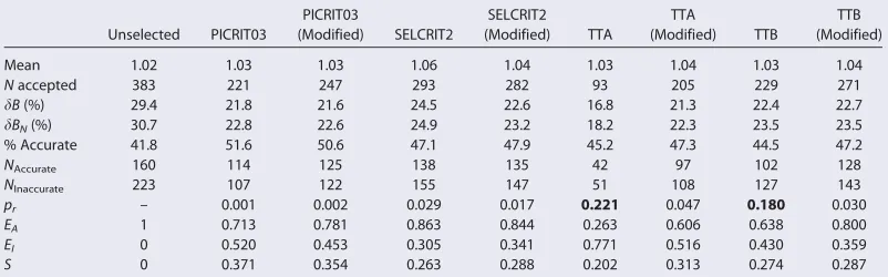
We reanalyze the paleointensity estimates that were published in the original studies. This analysis includes results that both passed and failed any subsequent data selection and should not be biased by any selec-tion criteria. Given that the original authors did not publish best-fits for the data fromMuxworthy[1998] andKrasa et al . [2003], and for one specimen fromYamamoto and Hoshi[2008], these data are excluded from this reanalysis. The descriptive statistics of the data set before and after the application of the four cri-teria sets are given in Table 3. Before selection cricri-teria are applied, the mean result is accurate (within a fac-tor 1.1 of the expected value), the scatter (dBN(%)) is29% of the mean and42% of all results are accurate. After applying the four unmodified criteria sets, all mean results are accurate and the scatters are reduced by6–12% with respect to the unselected data. Although all criteria increase the proportion of accurate results accepted, with the exception of PICRIT03,<50% of the accepted results are accurate. The unmodified PICRIT03 and SELCRIT2 are effective at significantly increasing the acceptance of accurate results (pr<0.05; Table 3). For both ThellierTool sets, however,pr0.180 and we cannot reject the null hypothesis that the proportions of accurate results accepted occurred by chance.

The modifications to PICRIT03 and SELCRIT2 make only a small difference to the final results (Table 3). The modified TTA criteria, however, represent a large improvement over the unmodified version. Despite a decrease in the efficiency of rejecting inaccurate results (EIdecreases), the overall score of the TTA criteria increases from 0.202 to 0.313 (due to the efficiency of accepting accurate results more than doubling). The modified criteria increase the proportion of accurate results accepted (2%) and are more effective than a random selection process (pr<0.05). For TTB, the modifications increase the proportion of accurate results accepted by2.5% over the original criteria andprdecreases from 0.180 to 0.030, which indicates that the modified criteria are a significant improvement over random selection and the original criteria set. The over-all score of the TTB criteria increases from 0.274 to 0.287 due to the improved acceptance of accurate results.

4.2. A Bootstrap Approach

[image:6.630.183.584.124.249.2]

The above results rely on reanalyzing previously published fits, which may suffer from user bias and may not represent the general behavior of a specimen and hence the true effectiveness of the selection criteria. To overcome this we adopt a bootstrap approach. For each specimen, a best fit segment is randomly fitted

Table 3.Descriptive Statistic of the Reanalyzed Published Fits Before and After the Application of Commonly Used Selection Criteria Setsa

Unselected PICRIT03

PICRIT03

(Modified) SELCRIT2

SELCRIT2 (Modified) TTA

TTA

(Modified) TTB

TTB (Modified)

Mean 1.02 1.03 1.03 1.06 1.04 1.03 1.04 1.03 1.04

Naccepted 383 221 247 293 282 93 205 229 271

dB(%) 29.4 21.8 21.6 24.5 22.6 16.8 21.3 22.4 22.7

dBN(%) 30.7 22.8 22.6 24.9 23.2 18.2 22.3 23.5 23.5

% Accurate 41.8 51.6 50.6 47.1 47.9 45.2 47.3 44.5 47.2

NAccurate 160 114 125 138 135 42 97 102 128

NInaccurate 223 107 122 155 147 51 108 127 143

pr – 0.001 0.002 0.029 0.017 0.221 0.047 0.180 0.030

EA 1 0.713 0.781 0.863 0.844 0.263 0.606 0.638 0.800

EI 0 0.520 0.453 0.305 0.341 0.771 0.516 0.430 0.359

S 0 0.371 0.354 0.263 0.288 0.202 0.313 0.274 0.287

a

(7)

to the Arai plot data. To ensure a physically reasonably ﬁt, the segment must contain at least three consecu-tive Arai plot points that deﬁne a segment with a negaconsecu-tive slope, it must have a gap factor (g)>0, and

f0.05. The random fitting process for each specimen is repeated until a best fit segment passing these conditions is found. This fitting procedure is repeated for all specimens to obtain a pseudo-data set of 395 paleointensity estimates and statistics. The various selection criteria sets are then applied to this pseudo-data set and the descriptive statistics recorded. This whole process is repeated for 104_{bootstraps to build} up distributions for the descriptive statistics of the pseudo-data sets before and after selection. All 395 specimens in Table 1 are included in this analysis.

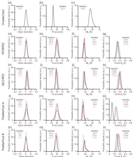
The probability densities for the descriptive statistics before and after selection are shown in Figure 1. Before selection the mean values from all the pseudo-data sets are accurate (|mean deviation|ln(1.1); Fig-ure 1a). The percentage of accurate results, however, is generally low (median32%) and the scatter high (median44%). In all cases, after selection there is a shift to higher proportions of accurate results in the accepted pseudo-data sets and a reduction in scatter. For PICRIT03 and SELCRIT2, the original and modified criteria behave similarly. The score for the modified PICRIT03 criteria is slightly higher than for the original (Figure 1g), but tends to be slightly lower for the modified SELCRIT2 when compared with the original crite-ria (Figure 1k).

Although more peaked around the median values, the mean deviations, the percentage of accurate results and the scatter of the modified TTA criteria behave similarly to the original (Figure 1l–1n). There is, however, a large increase in the scores of the selected data sets when the modified criteria are compared with the original criteria (median scores of 0.260 and 0.107, respectively; Figure 1o). As is the case for the analysis of the published fits, this large increase is due to a large increase inEA(theEAandEIdistributions are discussed in section 5). For the TTB criteria (Figure 1p–1s), both the original and modified criteria consistently yield accurate mean results and have similar proportions of accurate results (Figure 1q). The scatter remains unaf-fected by the modifications, but there is an increase in the scores of the modified TTB criteria with respect to the original set (Figure 1s).

The results of adding a quantitative curvature criterion to the modified criteria are represented by the gray dotted lines in Figure 1. In all cases, the distribution of the deviation of the mean values from the expected values becomes more peaked close to zero. For the proportion of accurate results in the accepted data sets, the addition ofj~kjincreases this percentage above all of the original criteria and improves on the modified criteria. The most notable difference after includingj~kjis the reduction of the scatter: The median values are reduced by2–5% with respect to both the original and modified criteria and is most pronounced for the SELCRIT2 and TTB criteria. Curved Arai plots can produce a wide range of values that both over and underestimate the expected paleointensity, whereas near-linear Arai plots yield only a narrow range of val-ues. It is the exclusion of this wide range of possible values from curved Arai plots that results in lower scatters.

The percentage of bootstrap results that yieldprvalue>0.05 (i.e., bootstrap results where the selection pro-cess cannot be distinguished from random selection) are shown in Table 4. For the original and modified PICRIT03 and SELCRIT2 criteria, these percentages are low (0.49%), which indicates that these criteria are effective at improving the acceptance of accurate results. The TTB criteria are moderately effective in their original form, with5.6% of the bootstraps yieldingpr>0.05. This is further reduced (0.95%) by the modi-fications suggested here. The TTA criteria are much less effective, with one in four bootstraps (26.02%) yield-ing results that are no better than random chance. The modified criteria greatly reduce this to 1.93% of bootstraps and the inclusion of a curvature criterion reduces this further (1.37%).

5. Discussion

(8)

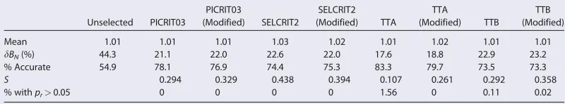
score. The main difference when using a relaxed deﬁnition of accuracy is in the percentage of bootstraps where the criteria are statistically indistinguishable from randomly selecting data. For PICRIT03, SELCRIT2, and TTB, before and after modiﬁcation the percentages remain low using a factor of 1.2 (Table 5). The

0 10 20

Probabilty density (a.u.)

0 25 50 75 100 % accurate (b)

0 10

5

δBN (%)

0 25 50 75

(c)

0 20 30

10

-0.2 -0.1 0 0.1 0.2

Mean deviation (a)

Unselected

0 5 10

% accurate (m)

0 25 50 75 100 0 10 20

δBN (%) (n)

0 25 50 75

Score (EA×EI) 0 5 20 15 10 (o)

0 0.2 0.4 0.6 0.8 0

20 30

10

Mean deviation (l)

-0.2 -0.1 0 0.1 0.2

ThellierTool A

0 12

6

% accurate (i)

0 25 50 75 100 0 20

10

δBN (%) (j)

0 25 50 75

Score (EA×EI) 0

15

10

5 (k)

0 0.2 0.4 0.6 0.8 0

24 36

12

Mean deviation (h)

-0.2 -0.1 0 0.1 0.2

SELCRIT2

0 5 10

% accurate (e)

0 25 50 75 100 0 10 20

δBN (%) (f)

0 25 50 75

Score (EA×EI) 0

15

10

5 (g)

0 0.2 0.4 0.6 0.8 0

20 30

10 (d)

-0.2 -0.1 0 0.1 0.2

Mean deviation

PICRIT03

0 12

6

% accurate (q)

0 25 50 75 100 0 30

20

10

δBN (%) (r)

0 25 50 75

Score (EA×EI) 0

15

10

5 (s)

0 0.2 0.4 0.6 0.8 0

12 24 36

Mean deviation (p)

-0.2 -0.1 0 0.1 0.2

[image:8.630.82.547.96.645.2]

ThellierTool B

Median 1.01 Median 44.3 Median 32.4 Median 1.01 1.01 1.02 Median 21.1 22.0 20.4 Median 50.5 49.5 53.7 Median 0.301 0.332 0.301 Median 1.03 1.02 1.02 Median 22.6 22.0 18.8 Median 46.2 47.4 51.9 Median 0.402 0.377 0.348 Median 1.01 1.02 1.02 Median 17.6 18.8 16.1 Median 50.0 50.0 52.9 Median 0.107 0.260 0.233 Median 1.01 1.01 1.01 Median 22.9 23.2 18.0 Median 45.6 46.2 52.4 Median 0.287 0.350 0.329

(9)

original TTA criteria are not effective at isolating estimates that are within a factor of 1.1 of the expected result (Table 4), but they are effective at isolating results within a factor of 1.2 and only 1.56% of bootstraps are no better than ran-dom chance. Despite this improvement for the original TTA criteria, we still prefer to use the factor 1.1 in our definition of accuracy. First, this definition is used in at least five studies that do not involve the authors of this current work [Chauvin et al., 2005;Bowles et al., 2006;Yamamoto and Hoshi, 2008;Herrero-Bervera and Valet, 2009;Valet et al., 2010] and reflects the general view of the paleointensity community. Second, we have demonstrated that, for the data set compiled here, various sets of selection criteria can be effective in isolating results that are within a factor 1.1 of the expected values. In cases where criteria are ineffective (e.g., TTA), theoretically justified modifications can make these criteria effective at isolating accurate results.

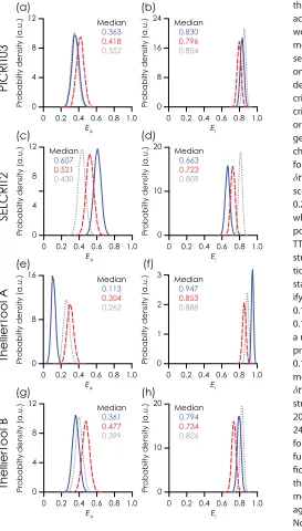
Throughout paleointensity literature, sets of selection criteria are variably described as strict or relaxed. The strictness and effectiveness of a set of selection criteria are a balance betweenEAandEI. Relaxed criteria tend to accept larger numbers of data and produce highEAvalues, but yield lowEIvalues. Conversely, strict criteria reject large numbers of data and tend to sacrificeEAto maximizeEI. By quantifyingEAandEI, we define relaxed selection criteria, whereEA>EI; strict selection criteria, whereEA<EI; and ideal criteria, where EA5EI51. The distributions ofEAandEIfrom the bootstrapped results are shown in Figure 2. In general, the sets of criteria tested here would be classified as strict (i.e.,EA<EI). This is most extreme for the original TTA criteria, where the medianEIis 0.947 (i.e., 94.7% of all inaccurate results are rejected), but the median EAis only 0.113 (11.3% of accurate results are accepted; Figures 2e and 2f). Although the TTA criteria are effective at rejecting inaccurate results they are ineffective are accepting accurate results, which is why in many cases they are no better than making a random selection of data. In this sense, the original TTA crite-ria are too strict. The modifications suggested here reduce the effectiveness of rejecting inaccurate results by a small amount, but allow for a relatively large increase in the acceptance of accurate results (Figure 2e). The other criteria sets are more balanced, in that they achieve highEIvalues while maintaining moderateEA values. For PICRIT03 and TTB, the modified criteria sets maintain or increase bothEAandEI(Figures 2a, 2b, 2g, and 2h). For SELCRIT2, the improved rejection of inaccurate results is offset by a reduction in the accep-tance of accurate results (lowerEA), which results in the small decrease in the overall score (Figure 1k). Despite this slight decrease, the theoretical basis for these modifications is a stronger justification for using the modified criteria.

While the modiﬁed criteria can improve the proportions of accurate results and increase the general effec-tiveness of accepting accurate results and rejecting inaccurate results (given byS), the scatters remain high (typically>20%). The addition of an experimentally constrained and quantitative measure of Arai plot cur-vature, however, can improve this. The addition ofj~kjreduces the overall scatter of the results through an improved rejection of inaccurate results (Figure 2). This is offset by a reduction inEA, but results in an overall improvement of the results when compared to the original criteria (Figure 1). We note that, althoughj~kjis one of only a few selection statistics that has been quantitatively constrained from independent control experiments, further work is needed to achieve the same level of theoretical understanding as has been achieved for the modiﬁcation based on SD predictions.

[image:9.630.184.383.111.169.2]

Of the original criteria sets investigated, the TTA criteria are the most ineffective at successfully isolating accurate results. This criteria set is widely used in the modern literature and, although the mean values of

Table 4.The Percentage of Bootstrapped Results Withpr>0.05

Original Modified Modified Incl.j~_k_j

PICRT03 0.49 0.28 0.10

SELCRIT2 0.06 0.22 0.07

TTA 26.02 1.93 1.37

[image:9.630.182.582.675.749.2]

TTB 5.64 0.95 0.02

Table 5.Median Values of the Descriptive Statistics From the Bootstrapped Data Set Using a Factor of 1.2 to Deﬁne Accurate Results

Unselected PICRIT03

PICRIT03

(Modified) SELCRIT2

SELCRIT2 (Modified) TTA

TTA

(Modified) TTB

TTB (Modified)

Mean 1.01 1.01 1.01 1.03 1.02 1.01 1.02 1.01 1.01

dBN(%) 44.3 21.1 22.0 22.6 22.0 17.6 18.8 22.9 23.2

% Accurate 54.9 78.1 76.9 74.4 75.3 83.3 79.7 73.5 73.3

S 0.294 0.329 0.438 0.394 0.107 0.261 0.292 0.358

(10)

the bootstrapped data set are accurate (Figure 1l), they have a worryingly high rate of being no more effective than randomly selecting data (Table 4). We rec-ommend that alternative, but demonstrably effective selection criteria, such as the modified TTA criteria be used instead of the original TTA criteria. Our sug-gested modifications make changes to threshold values for four statistics (f,dCK,dpal, and dt*), which results in the median score increasing from 0.107 to 0.260 (Figure 1o). To identify which statistic accounts for the poor performance of the original TTA criteria, we repeat the boot-strap process described in sec-tion 4.2, but modifying one statistic at a time. When we mod-ify onlyf, the median score is 0.132, fordCKthe median score is 0.126, modifying onlydpalyields a median score of 0.148, anddt* produces a median score of 0.124. For the four individual modifications (f,dCK,dpal, and dt*), the percentage of boot-straps wherepr>0.05, are 20.40%, 14.70%, 18.96%, and 24.19%, respectively (cf. 26.02% for the original and 1.93% for the fully modified criteria). The modi-fications todpalanddCKproduce the largest improvements to the median score and the percent-age of bootstraps withpr>0.05. No single modification, however, produces the large improvement seen from the fully modified cri-teria. The modifications are most effective when combined as a set, which indicates that multiple factors are influencing the data set compiled here. It also suggests that the interplay of different selection statistics is an important consideration when developing a better under-standing of how the data selection process works.

The poor performance of the original TTA criteria may not be isolated: Many studies use unique sets of selection criteria, the effectiveness of which remains unknown. Studies that use unique sets of selection cri-teria should define selection thresholds that fit with our latest quantitative understanding of how the selec-tion statistics behave, which may be derived from theoretical or empirical constraints. In addiselec-tion, we recommend that the effectiveness of selection criteria sets be assessed using a data set that is independent of how the criteria were defined and that provides a means to quantify the accuracy of the paleointensity results.

0 1 3

2

(f)

EI

0 0.2 0.4 0.6 0.8 1.0

0 16

8

(e)

EA

0 0.2 0.4 0.6 0.8 1.0

ThellierTool A

0 20

10

(d)

EI

0 0.2 0.4 0.6 0.8 1.0

0 4 8 12

(c)

EA

0 0.2 0.4 0.6 0.8 1.0

SELCRIT2

0 8 24

16

(b)

EI

0 0.2 0.4 0.6 0.8 1.0

0 8 12

4 (a)

EA

0 0.2 0.4 0.6 0.8 1.0

PICRIT03

0 20

10

(h)

EI

0 0.2 0.4 0.6 0.8 1.0

0 4 8 12

(g)

EA

0 0.2 0.4 0.6 0.8 1.0

[image:10.630.194.467.99.579.2]

ThellierTool B

Median 0.363 0.418 0.352 Median 0.830 0.796 0.854 Median 0.663 0.723 0.809 Median 0.113 0.304 0.262 Median 0.947 0.853 0.888 Median 0.361 0.477 0.399 Median 0.794 0.734 0.826 Median 0.607 0.521 0.430

Figure 2.Probability density functions ofEAandEIvalues from the bootstrapped data

(11)

In addition to the Coe and IZZI protocols, the original Thellier protocol [Thellier and Thellier, 1959] and the Aitken protocol [Aitken et al., 1988] are in current use.Paterson et al. [2012] andPaterson[2013] both dem-onstrated that whenBLab5BAncthe Aitken protocol behaves similarly to the Coe and IZZI protocols, but whenBLab>23BAncsome statistics deviate slightly from the Coe and IZZI trends. Nevertheless, the modifi-cations suggested here should be valid for the Aitken protocol, although without any data currently avail-able, we cannot test this. Similarly, modifications could be suggested for the criteria sets when applied to Thellier protocol data, however, in the absence of control data with which to assess the criteria sets we can-not test the validity of possible modifications.

6. Conclusions

Our ability to make reliable inferences about the ancient geomagnetic field strength relies heavily on con-sistently and reliably screening paleointensity data for nonideal behavior, but until now the efficacy of the data selection process has been unquantified. We have outlined the largest-to-date analysis of selection sta-tistics and presented a series of tools that allow the quantitative assessment of paleointensity data selec-tion. These tools have been used to assess the effectiveness of widely used criteria sets and the

effectiveness of modiﬁcations based on theoretical SD paleointensity behavior.

We have proposed a new standard document to define paleointensity data and help to remove ambiguities and inconsistencies that exist in data quantification. The Standard Paleointensity Definitions is intended to be a useful reference document for the paleomagnetic community. If readers have comments, suggestions, corrections, or criticisms, we warmly invite them to contact G.A.P. as all input that can help to further improve our ability to consistently select reliable paleointensity data is appreciated.

We have demonstrated that, when theoretical SD paleointensity behavior is considered, paleointensity data selection can be improved. This improvement comes in two forms. First, the modiﬁcations we propose can be used to improve the results of the data selection process and increase the likelihood of obtaining accu-rate and low scatter paleointensity estimates. Second, and importantly, these modiﬁcations are based on theoretical predictions that are derived independently of the large data set that we have compiled here. By taking this approach to modifying sets of paleointensity selection criteria we are beginning to place the data selection process on a more defensible theoretical foundation, which is essential for ensuring that we can reliably isolate accurate paleointensity data.

Despite this improvement, considerable work remains before we fully understand the quantitative manifes-tation of nonideal factors in selection statistics and whether or not they provide an effective means to screen these undesirable effects from our data sets. Although the necessary systematic studies can be difﬁ-cult and time consuming, the improvements that we see when applying a quantitative measure of Arai plot curvature demonstrate that they are a valuable undertaking.

We recommend that all sets of selection criteria used in future paleointensity studies follow some basic requirements to ensure the validity of the obtained results.

1. The threshold values used for selection must conform to the most recent quantitative understanding of selection statistic behavior, be this from theoretical considerations or from systematic control experiments that provide empirical constraints.

2. The efﬁcacy of selection criteria must be demonstrated using an independent data set, such as the one compiled here or any other relevant independent data set that allows the accuracy of results to be quantiﬁed.

3. The criteria should not exhibit a high proportion of instances where the average results are inaccurate with respect to an expected value or where the effectiveness of selection is no better than randomly select-ing data. We suggest that, in a bootstrap style test (cf., section 4.2), fewer than 5% of all bootstraps should yield results with an inaccurate mean and/orpr0.05.

For future studies, we strongly recommend the use of the modiﬁed criteria sets outlined here. These criteria sets ﬁt the above requirements and remove a large degree of arbitrariness from the selection of paleointensity data.

(12)

repositories, such as the MagIC database, which allow the raw paleointensity data to be stored and reana-lyzed as paleointensity data analysis develops, the usefulness of which is demonstrated here. Without such data availability, vast amounts of legacy data will be rendered unreliable, which will only hinder our ability to understand geomagnetic ﬁeld evolution.

References

Aitken, M. J., A. L. Allsop, G. D. Bussell, and M. B. Winter (1988), Determination of the intensity of the Earth’s magnetic ﬁeld during archaeo-logical times: Reliability of the Thellier technique,Rev. Geophys.,26, 3–12, doi:10.1029/RG026i001p00003.

Biggin, A. J. (2006), First-order symmetry of weak-ﬁeld partial thermoremanence in multi-domain (MD) ferromagnetic grains: 2. Implica-tions for Thellier-type palaeointensity determination,Earth Planet. Sci. Lett.,245, 454–470, doi:10.1016/j.epsl.2006.02.034.

Biggin, A. J., M. Perrin, and M. J. Dekkers (2007), A reliable absolute palaeointensity determination obtained from a non-ideal recorder,

Earth Planet. Sci. Lett.,257, 545–563, doi:10.1016/j.epsl.2007.03.017.

Biggin, A. J., S. Badejo, E. Hodgson, A. R. Muxworthy, J. Shaw, and M. J. Dekkers (2013), The effect of cooling rate on the intensity of ther-moremanent magnetization (TRM) acquired by assemblages of pseudo-single domain, multidomain and interacting single-domain grains,Geophys. J. Int.,193, 1239–1249, doi:10.1093/gji/ggt078.

Bowles, J., J. S. Gee, D. V. Kent, M. R. Perﬁt, S. A. Soule, and D. J. Fornari (2006), Paleointensity applications to timing and extent of eruptive activity, 9_–10_{N East Paciﬁc Rise,}_{Geochem. Geophys. Geosyst.}_,₇_{, Q06006, doi:10.1029/2005GC001141.}

Calvo-Rathert, M., A. Goguitchaichvili, M.-F. Bogalo, N. Vegas-Tubıa,A. Carrancho, and J. Sologashvili (2011), A paleomagnetic and paleointensity study on Pleistocene and Pliocene basaltic ﬂows from the Djavakheti Highland (Southern Georgia, Caucasus),Phys. Earth Planet. Inter.,187, 212–224, doi:10.1016/j.pepi.2011.03.008.

Chauvin, A., Y. Garcia, P. Lanos, and F. Laubenheimer (2000), Paleointensity of the geomagnetic ﬁeld recovered on archaeomagnetic sites from France,Phys. Earth Planet. Inter.,120, 111–136, doi:10.1016/S0031-9201(00)00148-5.

Chauvin, A., P. Roperch, and S. Levi (2005), Reliability of geomagnetic paleointensity data: The effects of the NRM fraction and concave-up behavior on paleointensity determinations by the Thellier method,Phys. Earth Planet. Inter.,150, 265–286, doi:10.1016/

j.pepi.2004.11.008.

Coe, R. S. (1967), Paleo-intensities of the Earth’s magnetic ﬁeld determined from Tertiary and Quaternary rocks,J. Geophys. Res.,72, 3247– 3262, doi:10.1029/JZ072i012p03247.

Coe, R. S., S. Gromme, and E. A. Mankinen (1978), Geomagnetic paleointensities from radiocarbon-dated lava ﬂows on Hawaii and the question of the Paciﬁc nondipole low,J. Geophys. Res.,83, 1740–1756, doi:10.1029/JB083iB04p01740.

Donadini, F., M. Kovacheva, M. Kostadinova, L. Casas, and L. J. Pesonen (2007), New archaeointensity results from Scandinavia and Bulgaria: Rock-magnetic studies inference and geophysical application,Phys. Earth Planet. Inter.,165, 229–247, doi:10.1016/j.pepi.2007.10.002. Herrero-Bervera, E., and J.-P. Valet (2009), Testing determinations of absolute paleointensity from the 1955 and 1960 Hawaiian ﬂows,Earth

Planet. Sci. Lett.,287, 420–433, doi:10.1016/j.epsl.2009.08.035.

Kissel, C., and C. Laj (2004), Improvements in procedure and paleointensity selection criteria (PICRIT-03) for Thellier and Thellier determina-tions: Application to Hawaiian basaltic long cores,Phys. Earth Planet. Inter.,147, 155–169, doi:10.1016/j.pepi.2004.06.010.

Krasa, D., C. Heunemann, R. Leonhardt, and N. Petersen (2003), Experimental procedure to detect multidomain remanence during Thellier-Thellier experiments,Phys. Chem. Earth,28, 681–687, doi:10.1016/S1474-7065(03)00122-0.

Leonhardt, R., C. Heunemann, and D. Krasa (2004), Analyzing absolute paleointensity determinations: Acceptance criteria and the software ThellierTool4.0,Geochem. Geophys. Geosyst.,5, Q12016, doi:10.1029/2004GC000807.

Muxworthy, A. R. (1998),Stability of Magnetic Remanence in Multidomain Magnetite, Univ. of Oxford, Oxford, U. K.

Muxworthy, A. R., D. Heslop, G. A. Paterson, and D. Michalk (2011), A Preisach method for estimating absolute paleoﬁeld intensity under the constraint of using only isothermal measurements: 2. Experimental testing,J. Geophys. Res.,116, B04103, doi:10.1029/ 2010JB007844.

Neukirch, L. P., J. A. Tarduno, T. N. Huffman, M. K. Watkeys, C. A. Scribner, and R. D. Cottrell (2012), An archeomagnetic analysis of burnt grain bin ﬂoors from ca. 1200 to 1250 AD Iron-Age South Africa,Phys. Earth Planet. Inter.,190–191, 71–79, doi:10.1016/

j.pepi.2011.11.004.

Paterson, G. A. (2011), A simple test for the presence of multidomain behaviour during paleointensity experiments,J. Geophys. Res.,116, B10104, doi:10.1029/2011JB008369.

Paterson, G. A. (2013), The effects of anisotropic and non-linear thermoremanent magnetizations on Thellier-type paleointensity data, Geo-phys. J. Int.,193, 694–710, doi:10.1093/gji/ggt033.

Paterson, G. A., D. Heslop, and A. R. Muxworthy (2010a), Deriving conﬁdence in paleointensity estimates,Geochem. Geophys. Geosyst.,11, Q07Z18, doi:10.1029/2010GC003071.

Paterson, G. A., A. R. Muxworthy, A. P. Roberts, and C. Mac Niocaill (2010b), Assessment of the usefulness of lithic clasts from pyroclastic deposits for paleointensity determination,J. Geophys. Res.,115, B03104, doi:10.1029/2009JB006475.

Paterson, G. A., A. J. Biggin, Y. Yamamoto, and Y. Pan (2012), Towards the robust selection of Thellier-type paleointensity data: The inﬂu-ence of experimental noise,Geochem. Geophys. Geosyst.,13, Q05Z43, doi:10.1029/2012GC004046.

Pick, T., and L. Tauxe (1993), Geomagnetic palaeointensities during the Cretaceous normal superchron measured using submarine basaltic glass,Nature,366, 238–242, doi:10.1038/366238a0.

Selkin, P. A., W. P. Meurer, A. J. Newell, J. S. Gee, and L. Tauxe (2000), The effect of remanence anisotropy on paleointensity estimates: A case study from the Archean Stillwater Complex,Earth Planet. Sci. Lett.,183, 403–416, doi:10.1016/S0012-821X(00)00292-2. Selkin, P. A., J. S. Gee, and L. Tauxe (2007), Nonlinear thermoremanence acquisition and implications for paleointensity data,Earth Planet.

Sci. Lett.,256, 81–89, doi:10.1016/j.epsl.2007.01.017.

Shaar, R., H. Ron, L. Tauxe, R. Kessel, A. Agnon, E. Ben-Yosef, and J. M. Feinberg (2010), Testing the accuracy of absolute intensity estimates of the ancient geomagnetic ﬁeld using copper slag material,Earth Planet. Sci. Lett.,290, 201–213, doi:10.1016/j.epsl.2009.12.022. Shaar, R., H. Ron, L. Tauxe, R. Kessel, and A. Agnon (2011), Paleomagnetic ﬁeld intensity derived from non-SD: Testing the Thellier IZZI

tech-nique on MD slag and a new bootstrap procedure,Earth Planet. Sci. Lett.,310, 213–224, doi:10.1016/j.epsl.2011.08.024.

Spassov, S., J.-P. Valet, D. Kondopoulou, I. Zananiri, L. Casas, and M. Le Goff (2010), Rock magnetic property and paleointensity determina-tion on historical Santorini lava ﬂows,Geochem. Geophys. Geosyst.,11, Q07006, doi:10.1029/2009GC003006.

Tanaka, H., Y. Hashimoto, and N. Morita (2012), Palaeointensity determinations from historical and Holocene basalt lavas in Iceland, Geo-phys. J. Int.,189, 833–845, doi:10.1111/j.1365-246X.2012.05412.x.

Acknowledgments

(13)

Tauxe, L., and H. Staudigel (2004), Strength of the geomagnetic ﬁeld in the Cretaceous Normal Superchron: New data from submarine basaltic glass of the Troodos Ophiolite,Geochem. Geophys. Geosyst.,5, Q02H06, doi:10.1029/2003GC000635.

Thellier, E., and O. Thellier (1959), Sur l’intensite du champ magnetique terrestre dans le passe historique et geologique,Ann. Geophys.,15, 285–376.

Valet, J.-P., E. Herrero-Bervera, J. Carlut, and D. Kondopoulou (2010), A selective procedure for absolute paleointensity in lava ﬂows, Geo-phys. Res. Lett.,37, L16308, doi:10.1029/2010GL044100.

Veitch, R. J., I. G. Hedley, and J.-J. Wagner (1984), An investigation of the intensity of the geomagnetic-ﬁeld during Roman times using mag-netically anisotropic bricks and tiles,Arch. Sci.,37, 359–373.

Yamamoto, Y., and H. Hoshi (2008), Paleomagnetic and rock magnetic studies of the Sakurajima 1914 and 1946 andesitic lavas from Japan: A comparison of the LTD-DHT Shaw and Thellier paleointensity methods,Phys. Earth Planet. Inter.,167, 118–143, doi:10.1016/ j.pepi.2008.03.006.

Yamamoto, Y., H. Tsunakawa, and H. Shibuya (2003), Palaeointensity study of the Hawaiian 1960 lava: Implications for possible causes of erroneously high intensities,Geophys. J. Int.,153, 263–276, doi:10.1046/j.1365-246X.2003.01909.x.