Data Mining
Know It All
AMSTERDAM • BOSTON • HEIDELBERG • LONDON NEW YORK • OXFORD • PARIS • SAN DIEGO SAN FRANCISCO • SINGAPORE • SYDNEY • TOKYO
Morgan Kaufmann is an imprint of Elsevier
Soumen Chakrabarti
Earl Cox
Eibe Frank
Ralf Hartmut Güting
Jaiwei Han
Xia Jiang
Micheline Kamber
Sam S. Lightstone
Morgan Kaufmann Publishers is an imprint of Elsevier. 30 Corporate Drive, Suite 400
Burlington, MA 01803
This book is printed on acid-free paper.
Copyright © 2009 by Elsevier Inc. All rights reserved.
Designations used by companies to distinguish their products are often claimed as trademarks or registered trademarks. In all instances in which Morgan Kaufmann Publishers is aware of a claim, the product names appear in initial capital or all capital letters. Readers, however, should contact the appropriate companies for more complete information regarding trademarks and registration.
No part of this publication may be reproduced, stored in a retrieval system, or transmitted in any form or by any means, electronic, mechanical, photocopying, scanning, or otherwise, without prior written permission of the publisher. Permissions may be sought directly from Elsevier’s Science & Technology Rights Department in Oxford, UK: phone: (+44) 1865 843830, fax: (+44) 1865 853333, e-mail: [email protected]. You may also complete your request on-line via the Elsevier homepage (http://elsevier.com), by selecting “Support & Contact” then “Copyright and Permission” and then “Obtaining Permissions.”
Library of Congress Cataloging-in-Publication Data Chakrabarti, Soumen.
Data mining: know it all / Soumen Chakrabarti et al. p. cm. — (Morgan Kaufmann know it all series) Includes bibliographical references and index. ISBN 978-0-12-374629-0 (alk. paper)
1. Data mining. I. Title. QA76.9.D343C446 2008
005.74—dc22 2008040367
For information on all Morgan Kaufmann publications, visit our Website at www.mkp.com or www.books.elsevier.com
Printed in the United States
08 09 10 11 12 10 9 8 7 6 5 4 3 2 1
Working together to grow
libraries in developing countries
Contents
About This Book ... ix
Contributing Authors ... xi
CHAPTER 1
What’s It All About?
... 11.1 Data Mining and Machine Learning ... 1
1.2 Simple Examples: The Weather Problem and Others ... 7
1.3 Fielded Applications ... 20
1.4 Machine Learning and Statistics ... 27
1.5 Generalization as Search ... 28
1.6 Data Mining and Ethics ... 32
1.7 Resources ... 34
CHAPTER 2
Data Acquisition and Integration
... 372.1 Introduction ... 37
2.2 Sources of Data ... 37
2.3 Variable Types... 39
2.4 Data Rollup ... 41
2.5 Rollup with Sums, Averages, and Counts ... 48
2.6 Calculation of the Mode ... 49
2.7 Data Integration ... 50
CHAPTER 3
Data Preprocessing
... 573.1 Why Preprocess the Data? ... 58
3.2 Descriptive Data Summarization ... 61
3.3 Data Cleaning ... 72
3.4 Data Integration and Transformation ... 78
3.5 Data Reduction ... 84
3.7 Summary ... 108
3.8 Resources ... 109
CHAPTER 4
Physical Design for Decision Support,
Warehousing, and OLAP
... 1134.1 What Is Online Analytical Processing? ... 113
4.2 Dimension Hierarchies ... 116
4.3 Star and Snowflake Schemas ... 117
4.4 Warehouses and Marts ... 119
4.5 Scaling Up the System ... 122
4.6 DSS, Warehousing, and OLAP Design Considerations ... 124
4.7 Usage Syntax and Examples for Major Database Servers ... 125
4.8 Summary ... 128
4.9 Literature Summary ... 129
Resources ... 129
CHAPTER 5
Algorithms: The Basic Methods
... 1315.1 Inferring Rudimentary Rules ... 132
5.2 Statistical Modeling ... 136
5.3 Divide and Conquer: Constructing Decision Trees ... 144
5.4 Covering Algorithms: Constructing Rules ... 153
5.5 Mining Association Rules ... 160
5.6 Linear Models ... 168
5.7 Instance-Based Learning ... 176
5.8 Clustering ... 184
5.9 Resources ... 188
CHAPTER 6
Further Techniques in Decision Analysis
... 1916.1 Modeling Risk Preferences ... 191
6.2 Analyzing Risk Directly ... 198
6.3 Dominance ... 200
6.4 Sensitivity Analysis ... 205
6.5 Value of Information ... 215
6.6 Normative Decision Analysis ... 220
CHAPTER 7
Fundamental Concepts of
Genetic Algorithms
... 2217.1 The Vocabulary of Genetic Algorithms ... 222
7.2 Overview ... 230
7.3 The Architecture of a Genetic Algorithm ... 241
7.5 Review ... 290
7.6 Resources ... 290
CHAPTER 8
Data Structures and Algorithms for Moving
Objects Types
... 2938.1 Data Structures ... 293
8.2 Algorithms for Operations on Temporal Data Types ... 298
8.3 Algorithms for Lifted Operations ... 310
8.4 Resources ... 319
CHAPTER 9
Improving the Model
... 3219.1 Learning from Errors ... 323
9.2 Improving Model Quality, Solving Problems ... 343
9.3 Summary ... 395
CHAPTER 10 Social Network Analysis
... 39710.1 Social Sciences and Bibliometry ... 398
10.2 PageRank and Hyperlink-Induced Topic Search ... 400
10.3 Shortcomings of the Coarse-Grained Graph Model ... 410
10.4 Enhanced Models and Techniques ... 416
10.5 Evaluation of Topic Distillation ... 424
10.6 Measuring and Modeling the Web ... 430
10.7 Resources ... 440
Index ... 443
About This Book
All of the elements about data mining are here together in a single resource written by the best and brightest experts in the field! This book consolidates both intro-ductory and advanced topics, thereby covering the gamut of data mining and machine learning tactics—from data integration and preprocessing to fundamental algorithms to optimization techniques and web mining methodology.
Contributing Authors
Soumen Chakrabarti (Chapter 10) is an associate professor of computer science and engineering at the Indian Institute of Technology in Bombay. He is also a popular speaker at industry conferences, the associate editor for ACM “Trans-actions on the Web,” as well as serving on other editorial boards. He is also the author of Mining the Web, published by Elsevier, 2003.
Earl Cox (Chapter 7) is the founder and president of Scianta Intelligence, a next-generation machine intelligence and knowledge exploration company. He is a futurist, author, management consultant, and educator dedicated to the epistemol-ogy of advanced intelligent systems, the redefinition of the machine mind, and the ways in which evolving and interconnected virtual worlds affect the sociology of business and culture. He is a recognized expert in fuzzy logic and adaptive fuzzy systems and a pioneer in the integration of fuzzy neural systems with genetic algorithms and case-based reasoning. He is also the author of Fuzzy Modeling and Genetic Algorithms for Data Mining Exploration, published by Elsevier, 2005.
Eibe Frank (Chapters 1 and 5) is a senior lecturer in computer science at the University of Waikato in New Zealand. He has published extensively in the area of machine learning and sits on editorial boards of the Machine Learning Journal and the Journal of Artificial Intelligence Research. He has also served on the programming committees of many data mining and machine learning conferences. He is the coauthor of Data Mining, published by Elsevier, 2005.
xii Contributing Authors
Jaiwei Han (Chapter 3) is director of the Intelligent Database Systems Research Laboratory and a professor at the School of Computing Science at Simon Fraser University in Vancouver, BC. Well known for his research in the areas of data mining and database systems, he has served on program committees for dozens of international conferences and workshops and on editorial boards for several journals, including IEEE Transactions on Knowledge and Data Engineering and Data Mining and Knowledge Discovery. He is also the coauthor of Data Mining: Concepts and Techniques, published by Elsevier, 2006.
Xia Jiang (Chapter 6) received an M.S. in mechanical engineering from Rose Hulman University and is currently a Ph.D. candidate in the Biomedical Informat-ics Program at the University of Pittsburgh. She has published theoretical papers concerning Bayesian networks, along with applications of Bayesian networks to biosurveillance. She is also the coauthor of Probabilistic Methods for Financial and Marketing Informatics, published by Elsevier, 2007.
Micheline Kamber (Chapter 3) is a researcher and freelance technical writer with an M.S. in computer science with a concentration in artificial intelligence. She is a member of the Intelligent Database Systems Research Laboratory at Simon Fraser University in Vancouver, BC. She is also the coauthor of Data Mining: Concepts and Techniques, published by Elsevier, 2006.
Sam S. Lightstone (Chapter 4) is the cofounder and leader of DB2’s autonomic computing R&D effort and has been with IBM since 1991. His current research interests include automatic physical database design, adaptive self-tuning resources, automatic administration, benchmarking methodologies, and system control. Mr. Lightstone is an IBM Master Inventor. He is also one of the coauthors of Physical Database Design, published by Elsevier, 2007.
Thomas P. Nadeau (Chapter 4) is a senior technical staff member of Ubiquiti Inc. and works in the area of data and text mining. His technical interests include data warehousing, OLAP, data mining, and machine learning. He is also one of the coauthors of Physical Database Design, published by Elsevier, 2007.
Richard E. Neapolitan (Chapter 6) is professor and Chair of Computer Science at Northeastern Illinois University. He is the author of Learning Bayesian Net-works (Prentice Hall, 2004), which ha been translated into three languages; it is one of the most widely used algorithms texts worldwide. He is also the coauthor of Probabilistic Methods for Financial and Marketing Informatics, published by Elsevier, 2007.
Contributing Authors xiii
and data surveying tools, and a self-adaptive modeling technology used in direct marketing applications. He is also a popular speaker at industry conferences, the associate editor for ACM “Transactions on Internet Technology,” and the author of Business Modeling and Data Mining (Morgan Kaufman, 2003).
Mamdouh Refaat (Chapter 2) is the director of Professional Services at ANGOSS Software Corporation. During the past 20 years, he has been an active member in the community, offering his services for consulting, researching, and training in various areas of information technology. He is also the author of Data Preparation for Data Mining Using SAS, published by Elsevier, 2007.
Markus Schneider (Chapter 8) is an assistant professor of computer science at the University of Florida, Gainesville, and holds a Ph.D. in computer Science from the University of Hagen in Germany. He is author of a monograph in the area of spatial databases, a German textbook on implementation concepts for database systems, coauthor of Moving Objects Databases (Morgan Kaufmann, 2005), and has published nearly 40 articles on database systems. He is on the editorial board of GeoInformatica.
Toby J. Teorey (Chapter 4) is a professor in the Electrical Engineering and Com-puter Science Department at the University of Michigan, Ann Arbor; his current research focuses on database design and performance of computing systems. He is also one of the coauthors of Physical Database Design, published by Elsevier, 2007.
CHAPTER
1
What’s It All About?
Human in vitro fertilization involves collecting several eggs from a woman’s ovaries, which, after fertilization with partner or donor sperm, produce several embryos. Some of these are selected and transferred to the woman’s uterus. The problem is to select the “best” embryos to use—the ones that are most likely to survive. Selection is based on around 60 recorded features of the embryos—char-acterizing their morphology, oocyte, follicle, and the sperm sample. The number of features is sufficiently large that it is difficult for an embryologist to assess them all simultaneously and correlate historical data with the crucial outcome of whether that embryo did or did not result in a live child. In a research project in England, machine learning is being investigated as a technique for making the selection, using as training data historical records of embryos and their outcome.
Every year, dairy farmers in New Zealand have to make a tough business deci-sion: which cows to retain in their herd and which to sell off to an abattoir. Typically, one-fifth of the cows in a dairy herd are culled each year near the end of the milking season as feed reserves dwindle. Each cow’s breeding and milk production history influences this decision. Other factors include age (a cow is nearing the end of its productive life at 8 years), health problems, history of dif-ficult calving, undesirable temperament traits (kicking or jumping fences), and not being in calf for the following season. About 700 attributes for each of several million cows have been recorded over the years. Machine learning is being inves-tigated as a way of ascertaining which factors are taken into account by successful farmers—not to automate the decision but to propagate their skills and experience to others.
Life and death. From Europe to the antipodes. Family and business. Machine learning is a burgeoning new technology for mining knowledge from data, a tech-nology that a lot of people are starting to take seriously.
1.1
DATA MINING AND MACHINE LEARNING
CHAPTER 1 What’s It All About?
computers make it too easy to save things that previously we would have trashed. Inexpensive multigigabyte disks make it too easy to postpone decisions about what to do with all this stuff—we simply buy another disk and keep it all. Ubiq-uitous electronics record our decisions, our choices in the supermarket, our financial habits, our comings and goings. We swipe our way through the world, every swipe a record in a database. The World Wide Web overwhelms us with information; meanwhile, every choice we make is recorded. And all these are just personal choices: they have countless counterparts in the world of commerce and industry. We would all testify to the growing gap between the generation of data and our understanding of it. As the volume of data increases, inexorably, the proportion of it that people understand decreases, alarmingly. Lying hidden in all this data is information, potentially useful information, that is rarely made explicit or taken advantage of.
This book is about looking for patterns in data. There is nothing new about this. People have been seeking patterns in data since human life began. Hunters seek patterns in animal migration behavior, farmers seek patterns in crop growth, politicians seek patterns in voter opinion, and lovers seek patterns in their part-ners’ responses. A scientist’s job (like a baby’s) is to make sense of data, to discover the patterns that govern how the physical world works and encapsulate them in theories that can be used for predicting what will happen in new situations. The entrepreneur’s job is to identify opportunities, that is, patterns in behavior that can be turned into a profitable business, and exploit them.
In data mining, the data is stored electronically and the search is automated— or at least augmented—by computer. Even this is not particularly new. Econo-mists, statisticians, forecasters, and communication engineers have long worked with the idea that patterns in data can be sought automatically, identified, vali-dated, and used for prediction. What is new is the staggering increase in oppor-tunities for finding patterns in data. The unbridled growth of databases in recent years, databases on such everyday activities as customer choices, brings data mining to the forefront of new business technologies. It has been estimated that the amount of data stored in the world’s databases doubles every 20 months, and although it would surely be difficult to justify this figure in any quantitative sense, we can all relate to the pace of growth qualitatively. As the flood of data swells and machines that can undertake the searching become commonplace, the opportunities for data mining increase. As the world grows in complexity, over-whelming us with the data it generates, data mining becomes our only hope for elucidating the patterns that underlie it. Intelligently analyzed data is a valuable resource. It can lead to new insights and, in commercial settings, to competitive advantages.
1.1 Data Mining and Machine Learning
those likely to switch products and those likely to remain loyal. Once such char-acteristics are found, they can be put to work to identify present customers who are likely to jump ship. This group can be targeted for special treatment, treatment too costly to apply to the customer base as a whole. More positively, the same techniques can be used to identify customers who might be attracted to another service the enterprise provides, one they are not presently enjoying, to target them for special offers that promote this service. In today’s highly competitive, customer-centered, service-oriented economy, data is the raw material that fuels business growth—if only it can be mined.
Data mining is defined as the process of discovering patterns in data. The process must be automatic or (more usually) semiautomatic. The patterns discov-ered must be meaningful in that they lead to some advantage, usually an economic advantage. The data is invariably present in substantial quantities.
How are the patterns expressed? Useful patterns allow us to make nontrivial predictions on new data. There are two extremes for the expression of a pattern: as a black box whose innards are effectively incomprehensible and as a transpar-ent box whose construction reveals the structure of the pattern. Both, we are assuming, make good predictions. The difference is whether or not the patterns that are mined are represented in terms of a structure that can be examined, reasoned about, and used to inform future decisions. Such patterns we call struc-tural because they capture the decision structure in an explicit way. In other words, they help to explain something about the data.
Now, finally, we can say what this book is about. It is about techniques for finding and describing structural patterns in data. Most of the techniques that we cover have developed within a field known as machine learning. But first let us look at what structural patterns are.
1.1.1
Describing Structural Patterns
What is meant by structural patterns? How do you describe them? And what form does the input take? We will answer these questions by way of illustration rather than by attempting formal, and ultimately sterile, definitions. We will present plenty of examples later in this chapter, but let’s examine one right now to get a feeling for what we’re talking about.
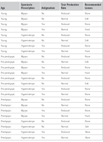
Look at the contact lens data in Table 1.1. This gives the conditions under which an optician might want to prescribe soft contact lenses, hard contact lenses, or no contact lenses at all; we will say more about what the individual features mean later. Each line of the table is one of the examples. Part of a structural description of this information might be as follows:
If tear production rate = reduced then recommendation = none Otherwise, if age = young and astigmatic = no
then recommendation = soft
CHAPTER 1 What’s It All About?
Table 1.1 The Contact Lens Data
Age Spectacle Prescription Astigmatism Tear Production Rate Recommended Lenses
Young Myope No Reduced None
Young Myope No Normal Soft
Young Myope Yes Reduced None
Young Myope Yes Normal Hard
Young Hypermetrope No Reduced None
Young Hypermetrope No Normal Soft
Young Hypermetrope Yes Reduced None
Young Hypermetrope Yes Normal Hard
Pre-presbyopic Myope No Reduced None
Pre-presbyopic Myope No Normal Soft
Pre-presbyopic Myope Yes Reduced None
Pre-presbyopic Myope Yes Normal Hard
Pre-presbyopic Hypermetrope No Reduced None
Pre-presbyopic Hypermetrope No Normal Soft
Pre-presbyopic Hypermetrope Yes Reduced None
Pre-presbyopic Hypermetrope Yes Normal None
Presbyopic Myope No Reduced None
Presbyopic Myope No Normal None
Presbyopic Myope Yes Reduced None
Presbyopic Myope Yes Normal Hard
Presbyopic Hypermetrope No Reduced None
Presbyopic Hypermetrope No Normal Soft
Presbyopic Hypermetrope Yes Reduced None
1.1 Data Mining and Machine Learning
be made and the resulting recommendation, are another popular means of expression.
This example is a simplistic one. First, all combinations of possible values are represented in the table. There are 24 rows, representing three possible values of age and two values each for spectacle prescription, astigmatism, and tear produc-tion rate (3 × 2 × 2 × 2 = 24). The rules do not really generalize from the data; they merely summarize it. In most learning situations, the set of examples given as input is far from complete, and part of the job is to generalize to other, new examples. You can imagine omitting some of the rows in the table for which tear production rate is reduced and still coming up with the rule
If tear production rate = reduced then recommendation = none
which would generalize to the missing rows and fill them in correctly. Second, values are specified for all the features in all the examples. Real-life datasets invari-ably contain examples in which the values of some features, for some reason or other, are unknown—for example, measurements were not taken or were lost. Third, the preceding rules classify the examples correctly, whereas often, because of errors or noise in the data, misclassifications occur even on the data that is used to train the classifier.
1.1.2
Machine Learning
Now that we have some idea about the inputs and outputs, let’s turn to machine learning. What is learning, anyway? What is machine learning? These are philo-sophic questions, and we will not be much concerned with philosophy in this book; our emphasis is firmly on the practical. However, it is worth spending a few moments at the outset on fundamental issues, just to see how tricky they are, before rolling up our sleeves and looking at machine learning in practice. Our dictionary defines “to learn” as follows:
n To get knowledge of by study, experience, or being taught. n To become aware by information or from observation. n To commit to memory.
n To be informed of, ascertain. n To receive instruction.
CHAPTER 1 What’s It All About?
instruction” seem to fall far short of what we might mean by machine learning. They are too passive, and we know that computers find these tasks trivial. Instead, we are interested in improvements in performance, or at least in the potential for performance, in new situations. You can “commit something to memory” or “be informed of something” by rote learning without being able to apply the new knowledge to new situations. You can receive instruction without benefiting from it at all.
Earlier we defined data mining operationally as the process of discovering patterns, automatically or semiautomatically, in large quantities of data—and the patterns must be useful. An operational definition can be formulated in the same way for learning:
Things learn when they change their behavior in a way that makes them per-form better in the future.
This ties learning to performance rather than knowledge. You can test learning by observing the behavior and comparing it with past behavior. This is a much more objective kind of definition and appears to be far more satisfactory.
But there’s still a problem. Learning is a rather slippery concept. Lots of things change their behavior in ways that make them perform better in the future, yet we wouldn’t want to say that they have actually learned. A good example is a comfortable slipper. Has it learned the shape of your foot? It has certainly changed its behavior to make it perform better as a slipper! Yet we would hardly want to call this learning. In everyday language, we often use the word “training” to denote a mindless kind of learning. We train animals and even plants, although it would be stretching the word a bit to talk of training objects such as slippers that are not in any sense alive. But learning is different. Learning implies thinking. Learning implies purpose. Something that learns has to do so intentionally. That is why we wouldn’t say that a vine has learned to grow round a trellis in a vine-yard—we’d say it has been trained. Learning without purpose is merely training. Or, more to the point, in learning the purpose is the learner’s, whereas in training it is the teacher’s.
Thus, on closer examination the second definition of learning, in operational, performance-oriented terms, has its own problems when it comes to talking about computers. To decide whether something has actually learned, you need to see whether it intended to or whether there was any purpose involved. That makes the concept moot when applied to machines because whether artifacts can behave purposefully is unclear. Philosophic discussions of what is really meant by “learn-ing,” like discussions of what is really meant by “intention” or “purpose,” are fraught with difficulty. Even courts of law find intention hard to grapple with.
1.1.3
Data Mining
pre-supposing any particular philosophic stance about what learning actually is. Data mining is a practical topic and involves learning in a practical, not a theoretic, sense. We are interested in techniques for finding and describing structural pat-terns in data as a tool for helping to explain that data and make predictions from it. The data will take the form of a set of examples—examples of customers who have switched loyalties, for instance, or situations in which certain kinds of contact lenses can be prescribed. The output takes the form of predictions about new examples—a prediction of whether a particular customer will switch or a prediction of what kind of lens will be prescribed under given circumstances. But because this book is about finding and describing patterns in data, the output may also include an actual description of a structure that can be used to classify unknown examples to explain the decision. As well as performance, it is helpful to supply an explicit representation of the knowledge that is acquired. In essence, this reflects both definitions of learning considered previously: the acquisition of knowledge and the ability to use it.
Many learning techniques look for structural descriptions of what is learned, descriptions that can become fairly complex and are typically expressed as sets of rules such as the ones described previously or the decision trees described later in this chapter. Because people can understand them, these descriptions explain what has been learned and explain the basis for new predictions. Experience shows that in many applications of machine learning to data mining, the explicit knowledge structures that are acquired, the structural descriptions, are at least as important, and often much more important, than the ability to perform well on new examples. People frequently use data mining to gain knowledge, not just predictions. Gaining knowledge from data certainly sounds like a good idea if you can do it. To find out how, read on!
1.2
SIMPLE EXAMPLES: THE WEATHER PROBLEM
AND OTHERS
We use a lot of examples in this book, which seems particularly appropriate con-sidering that the book is all about learning from examples! There are several standard datasets that we will come back to repeatedly. Different datasets tend to expose new issues and challenges, and it is interesting and instructive to have in mind a variety of problems when considering learning methods. In fact, the need to work with different datasets is so important that a corpus containing around 100 example problems has been gathered together so that different algorithms can be tested and compared on the same set of problems.
CHAPTER 1 What’s It All About?
with are intended to be “academic” in the sense that they will help us to under-stand what is going on. Some actual fielded applications of learning techniques are discussed in Section 1.3, and many more are covered in the books mentioned in the Further Reading section at the end of the chapter.
Another problem with actual real-life datasets is that they are often proprietary. No corporation is going to share its customer and product choice database with you so that you can understand the details of its data mining application and how it works. Corporate data is a valuable asset, one whose value has increased enor-mously with the development of data mining techniques such as those described in this book. Yet we are concerned here with understanding how the methods used for data mining work and understanding the details of these methods so that we can trace their operation on actual data. That is why our illustrations are simple ones. But they are not simplistic: they exhibit the features of real datasets.
1.2.1
The Weather Problem
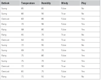
The weather problem is a tiny dataset that we will use repeatedly to illustrate machine learning methods. Entirely fictitious, it supposedly concerns the condi-tions that are suitable for playing some unspecified game. In general, instances in a dataset are characterized by the values of features, or attributes, that measure different aspects of the instance. In this case there are four attributes: outlook, temperature, humidity, and windy. The outcome is whether or not to play.
In its simplest form, shown in Table 1.2, all four attributes have values that are symbolic categories rather than numbers. Outlook can be sunny, overcast, or rainy; temperature can be hot, mild, or cool; humidity can be high or normal; and windy can be true or false. This creates 36 possible combinations (3 × 3 × 2 × 2 = 36), of which 14 are present in the set of input examples.
A set of rules learned from this information—not necessarily a very good one—might look as follows:
If outlook = sunny and humidity = high then play = no If outlook = rainy and windy = true then play = no If outlook = overcast then play = yes If humidity = normal then play = yes If none of the above then play = yes
These rules are meant to be interpreted in order: the first one; then, if it doesn’t apply, the second; and so on.
A set of rules intended to be interpreted in sequence is called a decision list. Interpreted as a decision list, the rules correctly classify all of the examples in the table, whereas taken individually, out of context, some of the rules are incorrect. For example, the rule if humidity = normal, then play = yes gets one of the examples wrong (check which one). The meaning of a set of rules depends on how it is interpreted—not surprisingly!
equality tests, as in the former case. This is called a numeric-attribute problem— in this case, a mixed-attribute problem because not all attributes are numeric.
Now the first rule given earlier might take the following form:
If outlook = sunny and humidity > 83 then play = no
A slightly more complex process is required to come up with rules that involve numeric tests.
The rules we have seen so far are classification rules: they predict the classi-fication of the example in terms of whether or not to play. It is equally possible to disregard the classification and just look for any rules that strongly associate different attribute values. These are called association rules. Many association rules can be derived from the weather data in Table 1.2. Some good ones are as follows:
If temperature = cool then humidity = normal If humidity = normal and windy = false then play = yes
If outlook = sunny and play = no then humidity = high If windy = false and play = no then outlook = sunny and humidity = high.
Table 1.2 The Weather Data
Outlook Temperature Humidity Windy Play
Sunny Hot High False No
Sunny Hot High True No
Overcast Hot High False Yes
Rainy Mild High False Yes
Rainy Cool Normal False Yes
Rainy Cool Normal True No
Overcast Cool Normal True Yes
Sunny Mild High False No
Sunny Cool Normal False Yes
Rainy Mild Normal False Yes
Sunny Mild Normal True Yes
Overcast Mild High True Yes
Overcast Hot Normal False Yes
Rainy Mild High True No
10 CHAPTER 1 What’s It All About?
All these rules are 100 percent correct on the given data; they make no false predictions. The first two apply to four examples in the dataset, the third to three examples, and the fourth to two examples. There are many other rules: in fact, nearly 60 association rules can be found that apply to two or more examples of the weather data and are completely correct on this data. If you look for rules that are less than 100 percent correct, then you will find many more. There are so many because unlike classification rules, association rules can “predict” any of the attributes, not just a specified class, and can even predict more than one thing. For example, the fourth rule predicts both that outlook will be sunny and that humidity will be high.
1.2.2
Contact Lenses: An Idealized Problem
[image:27.540.78.429.100.377.2]The contact lens data introduced earlier tells you the kind of contact lens to pre-scribe, given certain information about a patient. Note that this example is intended for illustration only: it grossly oversimplifies the problem and should certainly not be used for diagnostic purposes!
Table 1.3 Weather Data with Some Numeric Attribute
Outlook Temperature Humidity Windy Play
Sunny 85 85 False No
Sunny 80 90 True No
Overcast 83 86 False Yes
Rainy 70 96 False Yes
Rainy 68 80 False Yes
Rainy 65 70 True No
Overcast 64 65 True Yes
Sunny 72 95 False No
Sunny 69 70 False Yes
Rainy 75 80 False Yes
Sunny 75 70 True Yes
Overcast 72 90 True Yes
Overcast 81 75 False Yes
The first column of Table 1.1 gives the age of the patient. In case you’re won-dering, presbyopia is a form of longsightedness that accompanies the onset of middle age. The second gives the spectacle prescription: myope means short-sighted and hypermetrope means longsighted. The third shows whether the patient is astigmatic, and the fourth relates to the rate of tear production, which is important in this context because tears lubricate contact lenses. The final column shows which kind of lenses to prescribe: hard, soft, or none. All possible combinations of the attribute values are represented in the table.
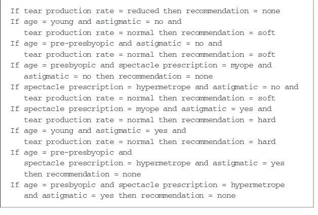
A sample set of rules learned from this information is shown in Figure 1.1. This is a large set of rules, but they do correctly classify all the examples. These rules are complete and deterministic: they give a unique prescription for every conceiv-able example. Generally, this is not the case. Sometimes there are situations in which no rule applies; other times more than one rule may apply, resulting in conflicting recommendations. Sometimes probabilities or weights may be associ-ated with the rules themselves to indicate that some are more important, or more reliable, than others.
[image:28.540.114.428.368.580.2]You might be wondering whether there is a smaller rule set that performs as well. If so, would you be better off using the smaller rule set and, if so, why? These are exactly the kinds of questions that will occupy us in this book. Because the examples form a complete set for the problem space, the rules do no more than summarize all the information that is given, expressing it in a different and more concise way. Even though it involves no generalization, this is often a useful
FIGURE 1.1
Rules for the contact lens data.
If tear production rate = reduced then recommendation = none If age = young and astigmatic = no and
tear production rate = normal then recommendation = soft If age = pre-presbyopic and astigmatic = no and
tear production rate = normal then recommendation = soft If age = presbyopic and spectacle prescription = myope and astigmatic = no then recommendation = none
If spectacle prescription = hypermetrope and astigmatic = no and tear production rate = normal then recommendation = soft If spectacle prescription = myope and astigmatic = yes and tear production rate = normal then recommendation = hard If age = young and astigmatic = yes and
tear production rate = normal then recommendation = hard If age = pre-presbyopic and
spectacle prescription = hypermetrope and astigmatic = yes then recommendation = none
If age = presbyopic and spectacle prescription = hypermetrope and astigmatic = yes then recommendation = none
1 CHAPTER 1 What’s It All About?
thing to do! People frequently use machine learning techniques to gain insight into the structure of their data rather than to make predictions for new cases. In fact, a prominent and successful line of research in machine learning began as an attempt to compress a huge database of possible chess endgames and their out-comes into a data structure of reasonable size. The data structure chosen for this enterprise was not a set of rules, but a decision tree.
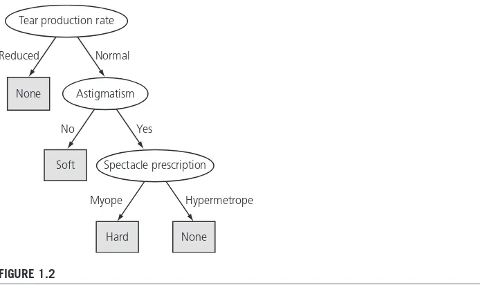
Figure 1.2 presents a structural description for the contact lens data in the form of a decision tree, which for many purposes is a more concise and perspicuous representation of the rules and has the advantage that it can be visualized more easily. (However, this decision tree—in contrast to the rule set given in Figure 1.1—classifies two examples incorrectly.) The tree calls first for a test on tear production rate, and the first two branches correspond to the two possible out-comes. If tear production rate is reduced (the left branch), the outcome is none. If it is normal (the right branch), a second test is made, this time on astigmatism. Eventually, whatever the outcome of the tests, a leaf of the tree is reached that dictates the contact lens recommendation for that case.
1.2.3
Irises: A Classic Numeric Dataset
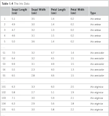
[image:29.540.79.428.78.284.2]The iris dataset, which dates back to seminal work by the eminent statistician R. A. Fisher in the mid-1930s and is arguably the most famous dataset used in data mining, contains 50 examples each of three types of plant: Iris setosa, Iris versi-color, and Iris virginica. It is excerpted in Table 1.4. There are four attributes: sepal length, sepal width, petal length, and petal width (all measured in centi-meters). Unlike previous datasets, all attributes have numeric values.
FIGURE 1.2
Decision tree for the contact lens data. Normal
Tear production rate
Reduced
Hypermetrope Myope
None Astigmatism
Soft
Hard None
Spectacle prescription Yes
Table 1.4 The Iris Data Sepal Length
(cm) Sepal Width (cm) Petal Length (cm) Petal Width (cm) Type
1 5.1 3.5 1.4 0.2 Iris setosa
2 4.9 3.0 1.4 0.2 Iris setosa
3 4.7 3.2 1.3 0.2 Iris setosa
4 4.6 3.1 1.5 0.2 Iris setosa
5 5.0 3.6 1.4 0.2 Iris setosa
. . .
51 7.0 3.2 4.7 1.4 Iris versicolor
52 6.4 3.2 4.5 1.5 Iris versicolor
53 6.9 3.1 4.9 1.5 Iris versicolor
54 5.5 2.3 4.0 1.3 Iris versicolor
55 6.5 2.8 4.6 1.5 Iris versicolor
. . .
101 6.3 3.3 6.0 2.5 Iris virginica
102 5.8 2.7 5.1 1.9 Iris virginica
103 7.1 3.0 5.9 2.1 Iris virginica
104 6.3 2.9 5.6 1.8 Iris virginica
105 6.5 3.0 5.8 2.2 Iris virginica
. . .
The following set of rules might be learned from this dataset:
If petal length < 2.45 then Iris setosa If sepal width < 2.10 then Iris versicolor
If sepal width < 2.45 and petal length < 4.55 then Iris versicolor If sepal width < 2.95 and petal width < 1.35 then Iris versicolor If petal length ≥ 2.45 and petal length < 4.45 then Iris versicolor If sepal length ≥ 5.85 and petal length < 4.75 then Iris versicolor If sepal width < 2.55 and petal length < 4.95 and
petal width < 1.55 then Iris versicolor
If petal length ≥ 2.45 and petal length < 4.95 and petal width < 1.55 then Iris versicolor
If sepal length ≥ 6.55 and petal length < 5.05 then Iris versicolor
1 CHAPTER 1 What’s It All About?
If sepal width < 2.75 and petal width < 1.65 and sepal length < 6.05 then Iris versicolor
If sepal length ≥ 5.85 and sepal length < 5.95 and petal length < 4.85 then Iris versicolor
If petal length ≥ 5.15 then Iris virginica If petal width ≥ 1.85 then Iris virginica
If petal width ≥ 1.75 and sepal width < 3.05 then Iris virginica If petal length ≥ 4.95 and petal width < 1.55 then Iris virginica
These rules are very cumbersome; more compact rules can be expressed that convey the same information.
1.2.4
CPU Performance: Introducing Numeric Prediction
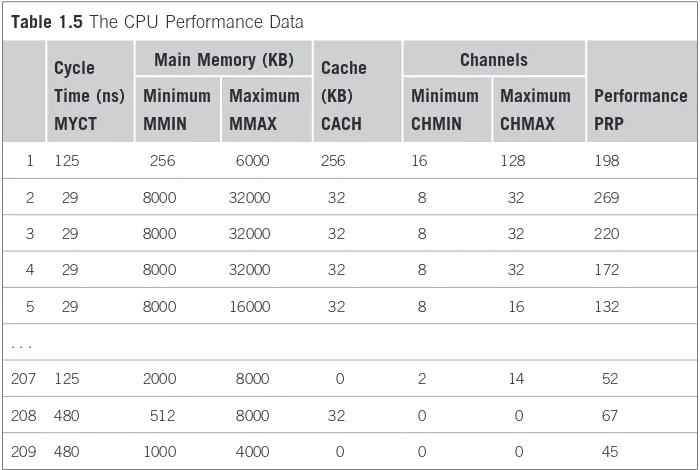
Although the iris dataset involves numeric attributes, the outcome—the type of iris—is a category, not a numeric value. Table 1.5 shows some data for which the outcome and the attributes are numeric. It concerns the relative performance of computer processing power on the basis of a number of relevant attributes; each row represents 1 of 209 different computer configurations.
The classic way of dealing with continuous prediction is to write the outcome as a linear sum of the attribute values with appropriate weights, for example:
PRP= − + MYCT+ MMIN+ MMAX+ CACH
−
55 9 0 0489 0 0153 0 0056 0 6410
0 27
. . . . .
[image:31.540.77.427.370.605.2]. 000CHMIN+1 480. CHMAX
Table 1.5 The CPU Performance Data
Cycle Main Memory (KB) Cache Channels
Time (ns) Minimum Maximum (KB) Minimum Maximum Performance
MYCT MMIN MMAX CACH CHMIN CHMAX PRP
1 125 256 6000 256 16 128 198
2 29 8000 32000 32 8 32 269
3 29 8000 32000 32 8 32 220
4 29 8000 32000 32 8 32 172
5 29 8000 16000 32 8 16 132
. . .
207 125 2000 8000 0 2 14 52
208 480 512 8000 32 0 0 67
(The abbreviated variable names are given in the second row of the table.) This is called a regression equation, and the process of determining the weights is called regression, a well-known procedure in statistics. However, the basic regres-sion method is incapable of discovering nonlinear relationships (although variants do exist).
In the iris and central processing unit (CPU) performance data, all the attributes have numeric values. Practical situations frequently present a mixture of numeric and nonnumeric attributes.
1.2.5
Labor Negotiations: A More Realistic Example
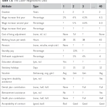
[image:32.540.113.465.256.606.2]The labor negotiations dataset in Table 1.6 summarizes the outcome of Canadian contract negotiations in 1987 and 1988. It includes all collective agreements
Table 1.6 The Labor Negotiations Data
Attribute Type 1 2 3 . . . 40
Duration Years 1 2 3 2
Wage increase first year Percentage 2% 4% 4.3% 4.5
Wage increase second year Percentage ? 5% 4.4% 4.0
Wage increase third year Percentage ? ? ? ?
Cost of living adjustment {none, tcf, tc} None Tcf ? None
Working hours per week Hours 28 35 38 40
Pension {none, ret-allw, empl-cntr} None ? ? ?
Standby pay Percentage ? 13% ? ?
Shift-work supplement Percentage ? 5% 4% 4
Education allowance {yes, no} Yes ? ? ?
Statutory holidays Days 11 15 12 12
Vacation {below-avg, avg, gen} Avg Gen Gen Avg
Long-term disability assistance
{yes, no} No ? ? Yes
Dental plan contribution {none, half, full} None ? Full Full
Bereavement assistance {yes, no} No ? ? Yes
Health plan contribution {none, half, full} None ? Full Half
Acceptability of contract {good, bad} Bad Good Good Good
1 CHAPTER 1 What’s It All About?
reached in the business and personal services sector for organizations with at least 500 members (teachers, nurses, university staff, police, etc.). Each case concerns one contract, and the outcome is whether the contract is deemed acceptable or unacceptable. The acceptable contracts are ones in which agreements were accepted by both labor and management. The unacceptable ones are either known offers that fell through because one party would not accept them or acceptable contracts that had been significantly perturbed to the extent that, in the view of experts, they would not have been accepted.
There are 40 examples in the dataset (plus another 17 that are normally reserved for test purposes). Unlike the other tables here, Table 1.6 presents the examples as columns rather than as rows; otherwise, it would have to be stretched over several pages. Many of the values are unknown or missing, as indicated by question marks.
This is a much more realistic dataset than the others we have seen. It contains many missing values, and it seems unlikely that an exact classification can be obtained.
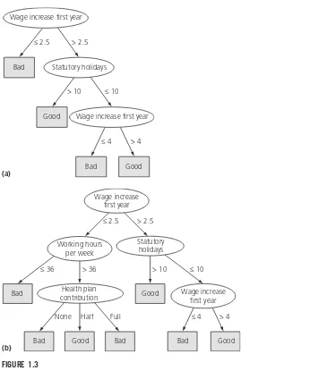
Figure 1.3 shows two decision trees that represent the dataset. Figure 1.3(a) is simple and approximate: it doesn’t represent the data exactly. For example, it will predict bad for some contracts that are actually marked good. But it does make intuitive sense: a contract is bad (for the employee!) if the wage increase in the first year is too small (less than 2.5 percent). If the first-year wage increase is larger than this, it is good if there are lots of statutory holidays (more than 10 days). Even if there are fewer statutory holidays, it is good if the first-year wage increase is large enough (more than 4 percent).
Figure 1.3(b) is a more complex decision tree that represents the same dataset. In fact, this is a more accurate representation of the actual dataset that was used to create the tree. But it is not necessarily a more accurate representation of the underlying concept of good versus bad contracts. Look down the left branch. It doesn’t seem to make sense intuitively that, if the working hours exceed 36, a contract is bad if there is no health-plan contribution or a full health-plan contribu-tion but is good if there is a half health-plan contribucontribu-tion. It is certainly reasonable that the health-plan contribution plays a role in the decision but not if half is good and both full and none are bad. It seems likely that this is an artifact of the par-ticular values used to create the decision tree rather than a genuine feature of the good versus bad distinction.
The tree in Figure 1.3(b) is more accurate on the data that was used to train the classifier but will probably perform less well on an independent set of test data. It is “overfitted” to the training data—it follows it too slavishly. The tree in Figure 1.3(a) is obtained from the one in Figure 1.3(b) by a process of pruning.
1.2.6
Soybean Classification: A Classic Machine Learning Success
FIGURE 1.3
Decision trees for the labor negotiations data. ≤ 2.5
Statutory holidays > 2.5
Bad
≤ 36
Health plan contribution > 36
Good > 10
Wage increase first year Wage increase
first year
Working hours per week
≤ 10
Bad None
Good Half
Bad Full
Bad ≤ 4
Good > 4
(b)
Wage increase first year
Bad ≤ 2.5
Statutory holidays > 2.5
Good > 10
Wage increase first year ≤ 10
Bad ≤ 4
Good > 4
(a)
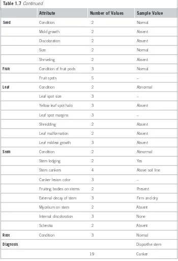
The data is taken from questionnaires describing plant diseases. There are about 680 examples, each representing a diseased plant. Plants were measured on 35 attributes, each one having a small set of possible values. Examples are labeled with the diagnosis of an expert in plant biology: there are 19 disease categories altogether—horrible-sounding diseases, such as diaporthe stem canker, rhizocto-nia root rot, and bacterial blight, to mention just a few.
1 CHAPTER 1 What’s It All About?
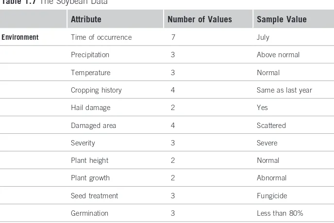
Table 1.7 gives the attributes, the number of different values that each can have, and a sample record for one particular plant. The attributes are placed into different categories just to make them easier to read.
Here are two example rules, learned from this data:
If [leaf condition is normal and stem condition is abnormal and stem cankers is below soil line and canker lesion color is brown] then
diagnosis is rhizoctonia root rot If [leaf malformation is absent and stem condition is abnormal and stem cankers is below soil line and canker lesion color is brown] then
diagnosis is rhizoctonia root rot
[image:35.540.81.425.376.606.2]These rules nicely illustrate the potential role of prior knowledge—often called domain knowledge—in machine learning, because the only difference between the two descriptions is leaf condition is normal versus leaf malformation is absent. In this domain, if the leaf condition is normal, then leaf malformation is necessarily absent, so one of these conditions happens to be a special case of the other. Thus, if the first rule is true, the second is necessarily true as well. The only time the second rule comes into play is when leaf malformation is absent
Table 1.7 The Soybean Data
Attribute Number of Values Sample Value
Environment Time of occurrence 7 July
Precipitation 3 Above normal
Temperature 3 Normal
Cropping history 4 Same as last year
Hail damage 2 Yes
Damaged area 4 Scattered
Severity 3 Severe
Plant height 2 Normal
Plant growth 2 Abnormal
Seed treatment 3 Fungicide
1. Simple Examples: The Weather Problem and Others 1
Table 1.7Continued
Attribute Number of Values Sample Value
Seed Condition 2 Normal
Mold growth 2 Absent
Discoloration 2 Absent
Size 2 Normal
Shriveling 2 Absent
Fruit Condition of fruit pods 3 Normal
Fruit spots 5 –
Leaf Condition 2 Abnormal
Leaf spot size 3 –
Yellow leaf spot halo 3 Absent
Leaf spot margins 3 –
Shredding 2 Absent
Leaf malformation 2 Absent
Leaf mildew growth 3 Absent
Stem Condition 2 Abnormal
Stem lodging 2 Yes
Stem cankers 4 Above soil line
Canker lesion color 3 –
Fruiting bodies on stems 2 Present
External decay of stem 3 Firm and dry
Mycelium on stem 2 Absent
Internal discoloration 3 None
Sclerotia 2 Absent
Root Condition 3 Normal
Diagnosis Diaporthe stem
0 CHAPTER 1 What’s It All About?
but leaf condition is not normal—that is, when something other than malforma-tion is wrong with the leaf. This is certainly not apparent from a casual reading of the rules.
Research on this problem in the late 1970s found that these diagnostic rules could be generated by a machine learning algorithm, along with rules for every other disease category, from about 300 training examples. The examples were carefully selected from the corpus of cases as being quite different from one another—”far apart” in the example space. At the same time, the plant pathologist who had produced the diagnoses was interviewed, and his expertise was trans-lated into diagnostic rules. Surprisingly, the computer-generated rules outper-formed the expert’s rules on the remaining test examples. They gave the correct disease top ranking 97.5 percent of the time compared with only 72 percent for the expert-derived rules. Furthermore, not only did the learning algorithm find rules that outperformed those of the expert collaborator, but the same expert was so impressed that he allegedly adopted the discovered rules in place of his own!
1.3
FIELDED APPLICATIONS
The examples that we opened with are speculative research projects, not pro-duction systems. And the preceding illustrations are toy problems: they are delib-erately chosen to be small so that we can use them to work through algorithms later in the book. Where’s the beef? Here are some applications of machine learn-ing that have actually been put into use.
Because they are fielded applications, the illustrations that follow tend to stress the use of learning in performance situations, in which the emphasis is on ability to perform well on new examples. This book also describes the use of learning systems to gain knowledge from decision structures that are inferred from the data. We believe that this is as important—probably even more important in the long run—a use of the technology as merely making high-performance predic-tions. Still, it will tend to be underrepresented in fielded applications because when learning techniques are used to gain insight, the result is not normally a system that is put to work as an application in its own right. Nevertheless, in three of the examples that follow, the fact that the decision structure is comprehensible is a key feature in the successful adoption of the application.
1.3.1
Decisions Involving Judgment
“accept” and “reject” cases. The remaining borderline cases are more difficult and call for human judgment. For example, one loan company uses a statistical deci-sion procedure to calculate a numeric parameter based on the information sup-plied in the questionnaire. Applicants are accepted if this parameter exceeds a preset threshold and rejected if it falls below a second threshold. This accounts for 90 percent of cases, and the remaining 10 percent are referred to loan officers for a decision. On examining historical data on whether applicants did indeed repay their loans, however, it turned out that half of the borderline applicants who were granted loans actually defaulted. Although it would be tempting simply to deny credit to borderline customers, credit industry professionals pointed out that if only their repayment future could be reliably determined it is precisely these customers whose business should be wooed; they tend to be active custom-ers of a credit institution because their finances remain in a chronically volatile condition. A suitable compromise must be reached between the viewpoint of a company accountant, who dislikes bad debt, and that of a sales executive, who dislikes turning business away.
Enter machine learning. The input was 1000 training examples of borderline cases for which a loan had been made that specified whether the borrower had finally paid off or defaulted. For each training example, about 20 attributes were extracted from the questionnaire, such as age, years with current employer, years at current address, years with the bank, and other credit cards possessed. A machine learning procedure was used to produce a small set of classification rules that made correct predictions on two-thirds of the borderline cases in an indepen-dently chosen test set. Not only did these rules improve the success rate of the loan decisions, but the company also found them attractive because they could be used to explain to applicants the reasons behind the decision. Although the project was an exploratory one that took only a small development effort, the loan company was apparently so pleased with the result that the rules were put into use immediately.
1.3.2
Screening Images
Since the early days of satellite technology, environmental scientists have been trying to detect oil slicks from satellite images to give early warning of ecologic disasters and deter illegal dumping. Radar satellites provide an opportunity for monitoring coastal waters day and night, regardless of weather conditions. Oil slicks appear as dark regions in the image whose size and shape evolve depending on weather and sea conditions. However, other look-alike dark regions can be caused by local weather conditions such as high wind. Detecting oil slicks is an expensive manual process requiring highly trained personnel who assess each region in the image.
CHAPTER 1 What’s It All About?
users—government agencies and companies—with different objectives, applica-tions, and geographic areas, it needs to be highly customizable to individual cir-cumstances. Machine learning allows the system to be trained on examples of spills and nonspills supplied by the user and lets the user control the trade-off between undetected spills and false alarms. Unlike other machine learning appli-cations, which generate a classifier that is then deployed in the field, here it is the learning method itself that will be deployed.
The input is a set of raw pixel images from a radar satellite, and the output is a much smaller set of images with putative oil slicks marked by a colored border. First, standard image processing operations are applied to normalize the image. Then, suspicious dark regions are identified. Several dozen attributes are extracted from each region, characterizing its size, shape, area, intensity, sharpness and jag-gedness of the boundaries, proximity to other regions, and information about the background in the vicinity of the region. Finally, standard learning techniques are applied to the resulting attribute vectors.
Several interesting problems were encountered. One is the scarcity of training data. Oil slicks are (fortunately) very rare, and manual classification is extremely costly. Another is the unbalanced nature of the problem: of the many dark regions in the training data, only a small fraction are actual oil slicks. A third is that the examples group naturally into batches, with regions drawn from each image forming a single batch, and background characteristics vary from one batch to another. Finally, the performance task is to serve as a filter, and the user must be provided with a convenient means of varying the false-alarm rate.
1.3.3
Load Forecasting
In the electricity supply industry, it is important to determine future demand for power as far in advance as possible. If accurate estimates can be made for the maximum and minimum load for each hour, day, month, season, and year, utility companies can make significant economies in areas such as setting the operating reserve, maintenance scheduling, and fuel inventory management.
and are each modeled separately by averaging hourly loads for that day over the past 15 years. Minor official holidays, such as Columbus Day, are lumped together as school holidays and treated as an offset to the normal diurnal pattern. All of these effects are incorporated by reconstructing a year’s load as a sequence of typical days, fitting the holidays in their correct position, and denormalizing the load to account for overall growth.
Thus far, the load model is a static one, constructed manually from historical data, and implicitly assumes “normal” climatic conditions over the year. The final step was to take weather conditions into account using a technique that locates the previous day most similar to the current circumstances and uses the historical information from that day as a predictor. In this case the prediction is treated as an additive correction to the static load model. To guard against outliers, the 8 most similar days are located and their additive corrections averaged. A database was constructed of temperature, humidity, wind speed, and cloud cover at three local weather centers for each hour of the 15-year historical record, along with the difference between the actual load and that predicted by the static model. A linear regression analysis was performed to determine the relative effects of these parameters on load, and the coefficients were used to weight the distance function used to locate the most similar days.
The resulting system yielded the same performance as trained human fore-casters but was far quicker—taking seconds rather than hours to generate a daily forecast. Human operators can analyze the forecast’s sensitivity to simulated changes in weather and bring up for examination the “most similar” days that the system used for weather adjustment.
1.3.4
Diagnosis
Diagnosis is one of the principal application areas of expert systems. Although the handcrafted rules used in expert systems often perform well, machine learning can be useful in situations in which producing rules manually is too labor intensive.
Preventative maintenance of electromechanical devices such as motors and generators can forestall failures that disrupt industrial processes. Technicians regularly inspect each device, measuring vibrations at various points to determine whether the device needs servicing. Typical faults include shaft misalignment, mechanical loosening, faulty bearings, and unbalanced pumps. A particular chem-ical plant uses more than 1000 different devices, ranging from small pumps to very large turbo-alternators, which until recently were diagnosed by a human expert with 20 years of experience. Faults are identified by measuring vibrations at different places on the device’s mounting and using Fourier analysis to check the energy present in three different directions at each harmonic of the basic rotation speed. The expert studies this information, which is noisy because of limitations in the measurement and recording procedure, to arrive at a diagno-sis. Although handcrafted expert system rules had been developed for some
CHAPTER 1 What’s It All About?
situations, the elicitation process would have to be repeated several times for dif-ferent types of machinery; so a learning approach was investigated.
Six hundred faults, each comprising a set of measurements along with the expert’s diagnosis, were available, representing 20 years of experience in the field. About half were unsatisfactory for various reasons and had to be discarded; the remainder were used as training examples. The goal was not to determine whether or not a fault existed but to diagnose the kind of fault, given that one was there. Thus, there was no need to include fault-free cases in the training set. The mea-sured attributes were rather low level and had to be augmented by intermediate concepts, that is, functions of basic attributes, which were defined in consultation with the expert and embodied some causal domain knowledge. The derived attri-butes were run through an induction algorithm to produce a set of diagnostic rules. Initially, the expert was not satisfied with the rules because he could not relate them to his own knowledge and experience. For him, mere statistical evi-dence was not, by itself, an adequate explanation. Further background knowledge had to be used before satisfactory rules were generated. Although the resulting rules were complex, the expert liked them because he could justify them in light of his mechanical knowledge. He was pleased that a third of the rules coincided with ones he used himself and was delighted to gain new insight from some of the others.
Performance tests indicated that the learned rules were slightly superior to the handcrafted ones that the expert had previously elicited, and subsequent use in the chemical factory confirmed this result. It is interesting to note, however, that the system was put into use not because of its good performance but because the domain expert approved of the rules that had been learned.
1.3.5
Marketing and Sales
Some of the most active applications of data mining have been in the area of marketing and sales. These are domains in which companies possess massive volumes of precisely recorded data, data that—it has only recently been real-ized—is potentially extremely valuable. In these applications, predictions them-selves are the chief interest: the structure of how decisions are made is often completely irrelevant.
groups for whom new services are appropriate, such as a cluster of profitable, reliable customers who rarely get cash advances from their credit card except in November and December, when they are prepared to pay exorbitant interest rates to see them through the holiday season. In another domain, cellular phone com-panies fight churn by detecting patterns of behavior that could benefit from new services and then advertise such services to retain their customer base. Incentives provided specifically to retain existing customers can be expensive, and success-ful data mining allows them to be precisely targeted to those customers where they are likely to yield maximum benefit.
Market basket analysis is the use of association techniques to find groups of items that tend to occur together in transactions, typically supermarket checkout data. For many retailers, this is the only source of sales information that is available for data mining. For example, automated analysis of checkout data may uncover the fact that customers who buy beer also buy chips, a discovery that could be significant from the supermarket operator’s point of view (although rather an obvious one that probably does not need a data mining exercise to discover). Or it may come up with the fact that on Thursdays, customers often purchase diapers and beer together, an initially surprising result that, on reflection, makes some sense as young parents stock up for a weekend at home. Such information could be used for many purposes: planning store layouts, limiting special discounts to just one of a set of items that tend to be purchased together, offering coupons for a matching product when one of them is sold alone, and so on. There is enormous added value in being able to identify individual customer’s sales histories. In fact, this value is leading to a proliferation of discount cards or “loyalty” cards that allow retailers to identify individual customers whenever they make a purchase; the personal data that results will be far more valuable than the cash value of the discount. Identification of individual customers not only allows historical analysis of purchasing patterns but also permits precisely targeted special offers to be mailed out to prospective customers.
This brings us to direct marketing, another popular domain for data mining. Promotional offers are expensive and have an extremely low—but highly profit-able—response rate. Any technique that allows a promotional mailout to be more tightly focused, achieving the same or nearly the same response from a much smaller sample, is valuable. Commercially available databases containing demo-graphic information based on ZIP codes that characterize the associated neigh-borhood can be correlated with information on existing customers to find a socioeconomic model that predicts what kind of people will turn out to be actual customers. This model can then be used on information gained in response to an initial mailout, where people send back a response card or call an 800 number for more information, to predict likely future customers. Direct mail companies have the advantage over shopping mall retailers of having complete purchasing histories for each individual customer and can use data mining to determine those likely to respond to special offers. Targeted campaigns are cheaper than mass-marketed campaigns because companies save money by sending offers only to