Review of applied statistical methods for flood frequency analysis in Europe

(1)

(2)

Published by the Centre for Ecology & Hydrology on behalf of COST.

ISBN: 978-1-906698-36-2

(3)

European flood-frequency analysis in a changing environment iii

Preface

This report has been prepared as part of the COST Action ES0901 “European procedures

for flood frequency estimation (FloodFreq)”. The main objective of the FloodFreq COST

Action is to undertake a Pan-European comparison and evaluation of methods for flood

frequency estimation under the various climatologic and geographic conditions found in

Europe, and different levels of data availability.

The report has been prepared by Working Group 4 “Flood frequency estimation methods

and environmental change”. It provides a review of methods used and results of detection of

trends in observations and climate projections of extreme precipitation and flood frequency

in Europe.

More information about the COST Action ES0901 can be found at the FloodFreq website

(4)

(5)

Summary

The report presents a review of methods used in Europe for trend analysis, climate change projections and non-stationary analysis of extreme precipitation and flood frequency. In addition, main findings of the analyses are presented, including a comparison of trend analysis results and climate change projections. Existing guidelines in Europe on design flood and design rainfall estimation that incorporate climate change are reviewed. The report concludes with a discussion of research needs on non-stationary frequency analysis for considering the effects of climate change and inclusion in design guidelines.

Trend analyses are reported for 21 countries in Europe with results for extreme precipitation, extreme streamflow or both. A large number of national and regional trend studies have been carried out. Most studies are based on statistical methods applied to individual time series of extreme precipitation or extreme streamflow using the non-parametric Mann-Kendall trend test or regression analysis. Some studies have been reported that use field significance or regional consistency tests to analyse trends over larger areas. Some of the studies also include analysis of trend attribution. The studies reviewed indicate that there is some evidence of a general increase in extreme precipitation, whereas there are no clear indications of significant increasing trends at regional or national level of extreme streamflow. For some smaller regions increases in extreme streamflow are reported. Several studies from regions dominated by snowmelt-induced peak flows report decreases in extreme streamflow and earlier spring snowmelt peak flows.

Climate change projections have been reported for 14 countries in Europe with results for extreme precipitation, extreme streamflow or both. The review shows various approaches for producing climate projections of extreme precipitation and flood frequency based on alternative climate forcing scenarios, climate projections from available global and regional climate models, methods for statistical downscaling and bias correction, and alternative hydrological models. A large number of the reported studies are based on an ensemble modelling approach that use several climate forcing scenarios and climate model projections in order to address the uncertainty on the projections of extreme precipitation and flood frequency. Some studies also include alternative statistical downscaling and bias correction methods and hydrological modelling approaches. Most studies reviewed indicate an increase in extreme precipitation under a future climate, which is consistent with the observed trend of extreme precipitation. Hydrological projections of peak flows and flood frequency show both positive and negative changes. Large increases in peak flows are reported for some catchments with rainfall-dominated peak flows, whereas a general decrease in flood magnitude and earlier spring floods are reported for catchments with snowmelt-dominated peak flows. The latter is consistent with the observed trends.

(6)

(7)

Editors

Madsen, H.1*, Lawrence, D.2, Lang, M.3, Martinkova, M.4, Kjeldsen, T.R.5

*_{Corresponding author ([email protected])}

1 _{DHI, Hørsholm, Denmark}

2 _{Norwegian Water Resources and Energy Directorate, Oslo, Norway}

3 _{Irstea, UR HHLY, Lyon, France}

4 _{T. G. Masaryk Water Research Institute, Prague, Czech Republic}

5 _{Centre for Ecology & Hydrology, Wallingford, UK}

Contributors

Willems, P., KU Leuven, Hydraulics Division, Leuven, Belgium

Neykov, N., National Institute of Meteorology and Hydrology, Bulgarian Academy of Sciences, Sofia, Bulgaria

Balabanova, S., National Institute of Meteorology and Hydrology, Bulgarian Academy of Sciences, Sofia, Bulgaria

Toumazis, A., Dion Toumazis & Associates, Nicosia, Cyprus

David, V., Faculty of Civil Engineering, Czech Technical University, Prague, Czech Republic

Karsten Arnbjerg-Nielsen, DTU Environment, Technical University of Denmark, Denmark

Veijalainen, N., Finnish Environment Institute, Freshwater Centre, Helsinki, Finland

Renard, B., Irstea, UR HHLY, Lyon, France

Vidal, J.P., Irstea, UR HHLY, Lyon, France

Merz, B., Helmholtz Centre Potsdam – GFZ German Research Centre for Geosciences, Section Hydrology, Potsdam, Germany

Loukas, A., Department of Civil Engineering, University of Thessaly, Pedion Areos, Volos, Greece

Vasiliades, L., Department of Civil Engineering, University of Thessaly, Pedion Areos, Volos, Greece

Pistocchi, A., GECOsistema srl – Cesena, Italy and Regione Emilia Romagna – Autorità dei Bacini Regionali Romagnoli, Forlì, Italy

Kriaučiūnienė, J., Lithuanian Energy Institute, Lithuania Sarauskiene, D., Lithuanian Energy Institute, Lithuania

Wilson, D., Norwegian Water Resources and Energy Directorate, Oslo, Norway

Strupczewski, W., Department of Hydrology and Hydrodynamics, Institute of Geophysics, Polish Academy of Sciences, Poland

Romanowicz, R., Department of Hydrology and Hydrodynamics, Institute of Geophysics, Polish Academy of Sciences, Poland

Osuch, M., Department of Hydrology and Hydrodynamics, Institute of Geophysics, Polish Academy of Sciences, Poland

(8)

Szolgay, J., Department of Land and Water Resources Management, Faculty of Civil Engineering, Slovak University of Technology, Bratislava, Slovakia

Kohnová, S., Department of Land and Water Resources Management, Faculty of Civil Engineering, Slovak University of Technology, Bratislava, Slovakia

Kobold, M., Faculty of Civil and Geodetic Engineering, University of Ljubljana, Ljubljana, Slovenia

Šraj, M., Faculty of Civil and Geodetic Engineering, University of Ljubljana, Ljubljana, Slovenia

Brilly, M., Faculty of Civil and Geodetic Engineering, University of Ljubljana, Ljubljana, Slovenia

Mediero, L., Department of Civil Engineering, Hydraulic and Energy Engineering, Technical University of Madrid, Madrid, Spain

Garrote, L., Department of Civil Engineering, Hydraulic and Energy Engineering, Technical University of Madrid, Madrid, Spain

Hernebring, C., DHI, Göteborg, Sweden

Olsson, J., Swedish Meteorological and Hydrological Institute, Norrköping, Sweden

Yücel, I., Middle East Technical University, Civil Engineering Department, Ankara, Turkey

Onusluel Gül, G., Dokuz Eylul University, Department of Civil Engineering, Izmir, Turkey

Prudhomme, C., Centre for Ecology & Hydrology, Wallingford, UK

(9)

1 Introduction

1.1 COST Action ES0901 FloodFreq

The main objective of the COST Action ES0901 is to undertake a Pan-European comparison and evaluation of methods for flood frequency estimation under the various climatologic and geographic conditions found in Europe, and different levels of data availability. A scientific framework for assessing the ability of these methods to predict the impact of environmental change on future flood frequency characteristics (flood occurrence and magnitude) will be developed and tested. The findings of the Action will be disseminated as a set of guidelines for professionals involved in flood management in Europe.

The objective will be accomplished through a series of network activities involving experts working on related problems through-out Europe. Specifically, the Action will produce the following deliverables:

1. Make available access to high-quality pan-European standard datasets and test-beds (detailed datasets including rainfall and runoff).

2. Produce a review of state-of-the-art methods for flood frequency estimation (considering both European and non-European methods).

3. Develop a scientific framework for assessing and comparing the performance of different methods (including considerations of prediction uncertainty).

4. Provide European-wide assessment of methods using the compiled datasets.

5. Provide a scientific framework for assessing the influence of environmental change on the future flood frequency characteristics.

6. Provide guidelines on flood frequency estimation for European professionals involved in flood risk management.

The work is organised in four working groups:

WG1: Compile dataset and inventories of existing data and methods

WG2: Use of statistical methods for flood frequency estimation

WG3: Flood frequency analysis using rainfall-runoff methods

WG4: Flood frequency estimation methods and environmental change

1.2 WG4: Flood frequency estimation methods and environmental change

Standard statistical procedures for flood frequency analysis are based on the assumption of stationarity; that is, the extreme flood statistics do not change in time, and hence past observations can be considered as representative of future observations and thus used to estimate design flood events. In a changing environment the assumption of stationarity might not be applicable, and more advanced statistical methods are required that explicitly

accounts for the non-stationarity of extreme flood characteristics.

The main driver for this working group is climate change and its effect on flood frequency. Results from global and regional climate modelling studies have indicated that most parts of Europe will experience more frequent and more severe floods in the future. The scientific challenge is to downscale the projections from the climate models to operational tools enabling policy makers to assess the impact of climate change on a local scale. Besides climate related changes in flood frequencies also direct anthropogenic changes in the

hydrological regime (e.g. land use changes, urbanisation, and wetland draining) and river

infrastructure developments need to be addressed.

The EU Floods Directive (2007/60/EC) states that consideration should be given to the possible effects of climate change on flood hazard in flood risk assessment and

(12)

mapping; 2) detailed flood hazard and flood risk mapping for areas identified during the preliminary mapping; and 3) development of flood risk management plans. The potential effects of long-term environmental changes on flood risk, including climate change, are to be considered both in conjunction with preliminary flood risk mapping and development of flood risk management plans. One of the motivations for this directive was that the Water

Framework Directive (2000/60/EC) does not particularly focus on measures related to the reduction of flood risk or on changes in flood risk under a future climate.

The Floods Directive, however, implicitly assumes that information regarding likely climate change impacts on flood frequency is readily available from global and regional climate projections such as those described in the most recent IPCC report (IPCC, 2007). This is, however, generally not the case as these impacts represent a local response to a changing climate and often cannot be directly interpreted from, say, regional projections for changes in precipitation. In addition, floods represent hydrological extremes and therefore demand high quality, high resolution input data to relevant models and analyses. Thus, the Floods

Directive indirectly poses a rather pressing need for methods and tools for modelling and analyses, which will lead to projections for likely changes in flood frequency under a future climate.

A key component of the FloodFreq COST Action is to develop a scientific framework for assessing the impacts of environmental change on flood frequency characteristics. The framework will be based on analysis of trends in historical data, combined with projections of future climate conditions from global and regional climate models, and analysis of historical developments of human induced changes in hydrological and hydraulic conditions. Process-based modelling can be used to analyse human induced changes and isolate climatological changes in flood frequency characteristics. Powerful statistical tools are required to detect changes or trends in extreme flood characteristics and to model time dependent statistical properties. In addition, a changing environment calls for a completely new paradigm for risk-based design guidelines and standards.

WG 4 has the following deliverables:

1. Review of existing methods for detecting trends and shifts in time series of extreme precipitation and floods, and non-stationary flood frequency analysis. A list of methods for use in Europe will be identified.

2. Guidelines for development of regional procedures for flood frequency analysis in a changing environment under the different climatic conditions in Europe.

3. New framework for risk-based design under environmental change by introduction of non-stationary design estimates.

4. Collection of open-source computer programs for non-stationary flood frequency analysis.

1.3 Report structure

(13)

Table 1.1 List of countries and organisations that have contributed to this report.

Country Organisation(s)

Belgium KU Leuven, Hydraulics Division, Leuven

Bulgaria National Institute of Meteorology and Hydrology, Bulgarian Academy of Sciences, Sofia

Cyprus Dion Toumazis & Associates, Nicosia

Czech Republic T. G. Masaryk Water Research Institute, Prague

Faculty of Civil Engineering, Czech Technical University, Prague Denmark DTU Environment, Technical University of Denmark

DHI, Hørsholm

Finland Finnish Environment Institute, Freshwater Centre, Helsinki France Irstea, UR HHLY, Lyon

Germany Helmholtz Centre Potsdam – GFZ German Research Centre for Geosciences, Section Hydrology, Potsdam

Greece Department of Civil Engineering, University of Thessaly, Pedion Areos, Volos

Italy GECOsistema srl – Cesena, Italy and Regione Emilia Romagna – Autorità dei Bacini Regionali Romagnoli, Forlì

Lithuania Lithuanian Energy Institute

Norway Norwegian Water Resources and Energy Directorate, Oslo Poland Department of Hydrology and Hydrodynamics, Institute of

Geophysics, Polish Academy of Sciences

Slovakia Department of Land and Water Resources Management, Faculty of Civil Engineering, Slovak University of Technology, Bratislava Slovenia Faculty of Civil and Geodetic Engineering, University of

Ljubljana, Ljubljana

Spain Department of Civil Engineering, Hydraulic and Energy Engineering, Technical University of Madrid, Madrid

Sweden Swedish Meteorological and Hydrological Institute, Norrköping DHI, Göteborg

Turkey Middle East Technical University, Civil Engineering Department, Ankara

Dokuz Eylul University, Department of Civil Engineering, Izmir UK Centre for Ecology & Hydrology, Wallingford

Department of Geography, University of Liverpool

The summary section is divided in three parts where methods and results from the country reports are summarised and discussed. The three parts are:

• Trend detection and attribution of precipitation extremes and floods (Section 2)

• Projections of precipitation extremes and floods under future climate change (Section

3)

• Non-stationary flood frequency and risk analysis, including a review of current

guidelines in Europe and identified research gaps (Section 4)

The 19 country reports are given in Appendix A.

In addition, in Appendix B reports from three non-European countries (Australia, India and the United States) are provided. These reports have been collected by the World

Meteorological Organization (WMO) Commission for Hydrology as part of their 2008-2012 programme ‘Water, Climate and Risk Management’. The WMO Commission for Hydrology liaised with the FloodFreq project in June 2011 where it was decided to gather information from some WMO countries along the same lines as the reports being prepared by the

(14)

2 Trend detection and attribution

Detection of trends in hydro-meteorological time series and analysis of the main driving factors that can explain the trends is important for understanding the impact of

environmental change. Below is presented methods applied for trend detection and

attribution of extreme rainfall and floods, followed by a summary of the main results of trend analyses in Europe.

2.1 Methods

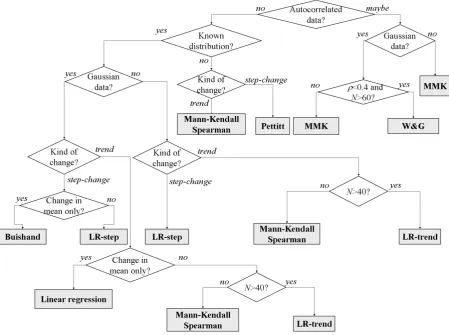
[image:14.595.73.523.280.615.2]

Several steps should be followed when performing a trend analysis. First, a preliminary analysis should be carried out to remove errors in data series (Section 2.1.1). The power of statistical trend tests is improved when longer time series data are used, but problems of measurement heterogeneity will affect the results, which especially may be a problem with old records. It is therefore important to work with data sets that have been quality controlled.

Figure 2.1 Flowchart for selection of a test for identifying trends and shifts in hydrological

extreme value series (from Lang et al., 2006). N: Sample size, ρ:

autocorrelation coefficient, LR: Likelihood ratio test, MMK: modified Mann-Kendall test, Buishand: test based on Buishand (1982).

(15)

Finally, when trends and shifts have been detected and considered significant, one should make an analysis of possible driving factors that can explain the changes, such as land-use change, river works, and climate change (Section 2.1.4).

2.1.1 Preliminary analysis to remove errors in data series

Examination of spatial homogeneity of rainfall data by detecting local anomalies is a

standard procedure performed by meteorological offices. Discharge data managers are also dealing with data control, especially in relation with the stability of the stage-discharge relationship, but such procedures cannot always ensure that the data series will be free of errors. It is therefore recommended to begin the trend detection analysis with a preliminary quality control of the data series.

The review reveals that some countries have implemented standard procedures for quality control of observed time series of precipitation and streamflow prior to trend analysis. In Greece, a methodology has been developed for automatic exploration and analysis of hydrological data, particularly focusing on the identification of changing relationships among hydrological variables. This method is applicable to many hydrological problems, such as identification of multiple stage-discharge relationships in a river section, data homogeneity analysis, analysis of temporal consistency of hydrological data, and detection of outliers (Tsakalias and Koutsoyiannis, 1999).

In Poland, measurement non-homogeneity, as a result of changes in measurement method or instrumentation, or time non-homogeneity, as a result of changes in the catchment conditions or river bed development over the observation period, is investigated using the Grubbs-Beck test (detection of outliers).

In Spain, the following procedure is applied:

• A graphical analysis is carried out at a local scale by plotting the cumulative annual

maximum discharge (AMD) for each station. Shifts are detected by changes in the slope of the cumulative graph.

• The discordance measure of Hosking and Wallis (1997) is computed at a regional

scale to identify stations that are grossly discordant with the group as a whole, taking advantage of the fact that trends and shifts in time series are reflected in the sample L-moments.

• Outliers are identified using the U.S. Water Resources Council method (USWRC,

1981). High outliers are removed from the AMD series and treated as historical data.

Homogeneity testing of the maximum discharge series from 70 hydrological stations in the

Baltic States (Estonia, Lithuania, Latvia) analysed in Reihan et al., (2007) was performed

using double-mass plot, correlation analysis, and the standard normal homogeneity test (Alexandersson and Moberg, 1997).

In Denmark, precipitation data are compared based on monthly averages between stations,

and extremes are verified against weather charts (Jørgensen et al., 1998).

2.1.2 Descriptive analysis of trends and shifts

Reported methods applied for analysing trends and shifts include both descriptive analyses and statistical tests. A simple descriptive approach is to compare distributions of extreme precipitation or discharge time series sampled from different sub-periods. For example, intensity-duration-frequency (IDF) curves for Nicosia, Cypress, were estimated and compared for two different periods, 1931-1970 (Hadjiioannou, 1995) and 1971-2007

(Pashiardis, 2009). Madsen et al. (2009) compared estimated regional IDF relationships for

Denmark (Madsen et al., 2002) for the periods 1979-1997 and 1979-2006.

(16)

Quantiles derived from the sub-periods were compared with quantiles derived from the full series (for given return periods), and the ratio of these quantiles defined a “quantile

anomaly”. The temporal (multi-decadal) variability of this anomaly was computed for a range

of rainfall durations. In the analysis of precipitation extremes in Northeastern Italy, Brunetti et

al. (2001) applied a 30-year moving window to estimate the trend in the frequency of

extreme precipitation events. In the Czech Republic, changes were analysed using a yearly index of flood regime related to seasonality and its variation with time (Šercl, 2009).

2.1.3 Testing for trends and shifts

Different statistical tests have been applied for testing for trends and shifts in extreme precipitation or discharge time series. These tests can be grouped into:

1. at-site tests that are applied to a single time series

2. field significance tests that are applied to multiple time series to test their joint statistical significance, and

3. regional consistency tests that are used for testing the spatial coherency of trends within a region.

At-site tests

At-site tests are statistical tests applied to individual time series. The most widely used test is the Mann-Kendall test, which has been applied to nationwide trend analysis studies of

extreme precipitation in Bulgaria (Bocheva et al., 2009), the Czech Republic (Kyselý, 2009)

and Denmark (Sadri et al., 2009), and to flood discharge in Finland (Korhonen and Kuusisto,

2010), Germany (Petrow and Merz, 2009; Petrow et al., 2009; Boormann et al., 2011),

Lithuania (Meilutyte-Barauskiene and Kovalenkovienė, 2007; Meilutyte-Barauskiene et al.,

2010), Slovenia (Jurko, 2009), and the UK (Hannaford and Marsh, 2008), and in two regional

studies for the Baltic (Reihan et al., 2007; Reihan et al., 2012) and the Nordic (Wilson et al.,

2010) countries. The modified Mann-Kendall test is recommended for auto-correlated data

(e.g. Korhonen and Kuusisto, 2010; Petrow and Merz, 2009; Petrow et al., 2009). In this

case trends can be quantified using the non-parametric linear Sen’s slope estimator (Sen,

1968), and if data are found to be auto-correlated, a pre-whitening procedure (e.g. Wang

and Swail, 2001; Yue et al, 2003) can be applied to remove autocorrelation from the time

series prior to applying the Mann-Kendall test.

Regression analysis has been applied to extreme precipitation series in Denmark

(Gregersen et al., 2010), Sweden (Bengtsson, 2011) and Greece (Nastos and Zerefos,

2008), and to flood discharge series in Germany (Bormann et al., 2011), Poland

(Strupczewski et al., 2009), Slovenia (Jurko, 2009), and the UK (Robson et al., 1998;

Hannaford and Marsh, 2008). Strupczewski et al. (2009) applied linear regression analysis to

both the mean and the variance of annual maximum flow series. In a study of extreme precipitation data in Thessaloniki, Greece Galiatsatou and Prinos (2007) applied polynomial regression of the estimated location and scale parameter of the Gumbel distribution.

Other applications of at-site trend tests that have been reported include Pettitt’s change point test and non-parametric sign test, which were applied to flood time series from Alpine basins in Switzerland by Castellarin and Pistocchi (2011); and normal scores regression and

Spearman’s correlation tests, which were applied to UK annual maximum and peak-over

threshold series by Robson et al. (1998).

In a French national study a number of different tests were compared, and a general

framework for selection of tests was developed (Renard, 2006; Lang et al., 2006), see

Figure 2.1. Parametric tests based on the likelihood ratio between two alternative

hypotheses (LR tests) appeared to be the most powerful, especially for extreme value data,

provided that the distributional assumptions (e.g. Generalized Extreme Value or Generalized

(17)

Field significance tests

Field significance is assessed when a statistical test is repeated on several individual time

series (e.g. from several locations in a given region) to test their joint significance and has

been studied, for example, by Livezey and Chen (1983), Lettenmaier et al. (1994), Douglas

et al. (2000), Yue and Wang (2002), Ventura et al. (2004), and Renard and Lang (2007). In a

trend and change detection context, it aims at testing the H0-hypothesis: “data from all sites are stationary”. Several methods accounting for dependence between the series have been proposed to assess the distribution of the number of locally significant tests under the H0-hypothesis, including (1) an equivalent (or effective) number of stations (ENS) (Matalas and

Langbein, 1962); (2) a bootstrap procedure (Douglas et al., 2000); (3) a Gaussian copula

methodology (Renard and Lang, 2007), and (4) the false discovery rate (FDR) (Benjamini

and Hochberg, 1995; Ventura et al., 2004).

In France, Renard et al. (2008) recommended the bootstrap procedure, as it is easier to

apply and requires no parametric assumption about marginal and joint distributions of the data. On the other hand, the FDR procedure is significantly more powerful for detecting changes affecting only a limited part of the sites, but is less powerful for detecting weaker generalized changes. Thus, the choice between the bootstrap and the FDR procedure depends on the expected type of change. When no prior information about the regional change is available, a pragmatic approach would simply consist in applying both tests to the data. In the trend analyses of flood time series in Germany by Petrow and Merz (2009) and

Petrow et al. (2009), field significance was evaluated by the bootstrap method of Douglas et

al. (2000), using a slightly modified approach in which field significance of upward and

downward trends are assessed separately (Yue et al., 2003). In the analysis of flood time

series in the Nordic countries Wilson et al. (2010) used the bootstrap procedure described

by Burn and Hag Elnur (2002) to determine the percentage of stations that are expected to show a trend due to the effect of cross-correlation between stations.

Regional consistency tests

Since climate change is likely to have an impact over large areas, river flows in nearby catchments located within the same homogenous climatic area are expected to be impacted by a similar change. Several methods have been developed to test for regional climate

changes: (1) univariate tests (e.g. Mann-Kendall test) of regional indices, i.e. variables

defined over the entire region (e.g. the regional mean value of the date of occurrence of the

annual maximum flood); (2) the regional average Mann-Kendall test proposed by Douglas et

al. (2000) and Yue and Wang (2002); (3) a semi-parametric approach based on a normal

score transformation and multivariate Gaussian distribution (Renard et al., 2008). In terms of

power, Renard et al. (2008) found no best method, but they recommended the

semi-parametric approach as it forces the regional trend to be consistent. Sadri et al. (2009)

applied the regional Mann-Kendall test to extreme precipitation data in Denmark.

2.1.4 Trend attribution

When trends or shifts have been detected, the next step in many studies is to analyse for the causes and attribute the changes to drivers such as climate change, land-use change, river developments, etc. Petrow and Merz (2009) analysed the spatial and seasonal patterns of changes in flood time series in Germany. They concluded that the spatial and seasonal coherence of the trends suggested that the observed changes in flood behaviour were

climate-driven. In a follow-up study, Petrow et al. (2009) related the trends in flood time

series to changes in circulation patterns and concluded that changes in the dynamics of

atmospheric circulations have an influence on the changes in floods. Bormann et al. (2011)

(18)

In the study of Alpine catchments in Switzerland, Allamano et al. (2009ab) proposed and applied a simple conceptual model that relates temperature regimes to the frequency of floods. They showed that an increase in the frequency of floods may be explained in terms

of temperature increases. The model of Allamano et al. (2009ab) was shown to be able to

explain observed trends in annual maxima series in alpine basins in Switzerland (Castellarin and Pistocchi, 2011). In the analysis of spring floods in the Baltic countries trends towards earlier and decreasing spring floods were found, which could be related to increasing

temperature (Meilutyte-Barauskiene and Kovalenkovienė, 2007; Reihan et al., 2007; Reihan

et al., 2012). Renard et al. (2008) applied a procedure developed by Andreassian et al.

(2003) to assess the relationship between rainfall and flow changes on four stations in the North-East of France.

Recently, Merz et al. (2012) argued that state-of-the-art trend analysis lack scientific rigour in

trend attribution and most attribution studies are based on qualitative reasoning or even speculation. They advocate for a statistically consistent approach for hypothesis testing of trend attribution and discuss ways forward to address this.

2.2 Summary of country review reports

The reported studies on trend analysis of extreme precipitation and flood frequency are summarised in Table 2.1. The summary includes information about:

1. Study location: nationwide, regional, specific river basins or catchments

2. Variable considered, i.e. precipitation (of given durations) or discharge time series, including information, if available, on No. of stations and length of the time series included in the analysis

3. Trend detection method(s) applied

4. Summary of key findings

5. References

A summary of the general findings and comparison with projected climate change in extreme precipitation and flood frequency is given in Section 3.3.

(19)

[image:19.595.85.485.47.330.2]

(20)

[image:20.842.96.742.90.524.2]

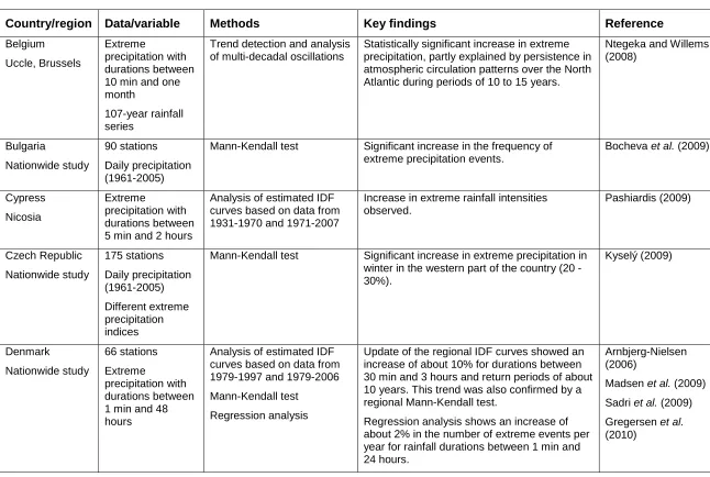
Table 2.1

Summary of country review reports on trend detection of precipitation extremes and flood frequency.

Country/region Data/variable Methods Key findings Reference

Belgium

Uccle, Brussels

Extreme

precipitation with durations between 10 min and one month

107-year rainfall series

Trend detection and analysis of multi-decadal oscillations

Statistically significant increase in extreme precipitation, partly explained by persistence in atmospheric circulation patterns over the North Atlantic during periods of 10 to 15 years.

Ntegeka and Willems (2008) Bulgaria Nationwide study 90 stations Daily precipitation (1961-2005)

Mann-Kendall test Significant increase in the frequency of extreme precipitation events.

Bocheva et al. (2009)

Cypress

Nicosia

Extreme

precipitation with durations between 5 min and 2 hours

Analysis of estimated IDF curves based on data from 1931-1970 and 1971-2007

Increase in extreme rainfall intensities observed. Pashiardis (2009) Czech Republic Nationwide study 175 stations Daily precipitation (1961-2005) Different extreme precipitation indices

Mann-Kendall test Significant increase in extreme precipitation in winter in the western part of the country (20 - 30%). Kyselý (2009) Denmark Nationwide study 66 stations Extreme precipitation with durations between 1 min and 48 hours

Analysis of estimated IDF curves based on data from 1979-1997 and 1979-2006

Mann-Kendall test

Regression analysis

Update of the regional IDF curves showed an increase of about 10% for durations between 30 min and 3 hours and return periods of about 10 years. This trend was also confirmed by a regional Mann-Kendall test.

Regression analysis shows an increase of about 2% in the number of extreme events per year for rainfall durations between 1 min and 24 hours.

Arnbjerg-Nielsen (2006)

Madsen et al. (2009) Sadri et al. (2009) Gregersen et al.

(21)

Finland

Nationwide study

25 stations

Daily discharge

Mann-Kendall test Earlier timing of spring peak flow observed at more than one third of the sites. However, no trend observed in the magnitudes of spring peak flow. Korhonen and Kuusisto (2010) France Nationwide study 195 stations Daily discharge

Field significance test

Semi-parametric regional consistency procedure

No general change was found at the national scale. Increased flood peaks were observed in Northeast, consistent with the trend in

observed rainfall.

A decreasing trend in high flow was observed in the Pyrenees. In the Alps, earlier snowmelt-related floods and increasing runoff due to glacier melting were observed.

Renard (2006) France Mediterranean region 92 stations Daily precipitation (1945–2004) Peak-over-threshold extreme value model with

non-stationary parameters

Statistically significant increase of the

occurrence and the intensity of extreme rainfall in three out of seven regions were detected.

Pujol et al. (2007)

Germany

Nationwide study

150 stations

Flood time series (1951-2002)

Mann-Kendall test

Field significance test (Douglas et al., 2000)

Trends in floods were detected for a considerable number of catchments (both positive and negative trends). Catchments with significant trends were spatially clustered, suggesting that the observed changes in flood behaviour are climate-driven.

Changes in circulation patterns were found to influence the changes in floods.

Petrow and Merz (2009)

Petrow et al. (2009)

Germany

Nationwide study

78 stations

Discharge and river levels

Chi-squared test on two-way contingency tables of flood versus non-flood years (Pinter et al., 2006).

Linear regression and Mann-Kendall test of annual maximum discharge

With respect to annual maximum discharge and flood frequency no significant trends could be identified consistently throughout the country. Significant trends in extreme discharge were identified at a number of stations (both positive and negative trends).

Bormann et al.

(2011) Greece Nationwide study 21 stations Daily precipitation (1957–2001)

Linear regression test of No. of days with precipitation above 50 mm

Increasing (but not significant) trend of the frequency of extreme precipitation

(22)

Greece

Thessaloniki

Daily precipitation (1958-2000)

Polynomial regression of estimated location and scale parameter in Gumbel distribution of annual maxima

No significant trends in the extreme value parameters were found.

Galiatsatou and Prinos (2007) Italy North-eastern Italy 7 stations Daily precipitation (1920–1998)

Frequency analysis of extreme events using a 30-year moving window

Increase in the frequency of extreme events. Brunetti et al. (2001)

Switzerland

Alpine basins

17 stations

Annual maximum discharge (91-140 years of record)

Pettitt’s change point test

Non-parametric sign test

Sen’s trend test

Significant changes in the frequency regime of annual maxima and increasing trends in the magnitude of annual flood peaks.

Castellarin and Pistocchi (2011) Lithuania Nationwide study 32 stations Daily discharge (1922-2003)

Mann-Kendall test Decrease in spring flood magnitude and trend towards an earlier spring flood throughout the country. Meilutyte-Barauskiene and Kovalenkovienė (2007)

Meilutyte-Barauskiene et al.

(2010) Baltic countries (Lithuania, Latvia, and Estonia) 70 stations Daily discharge (84 years of record)

Mann-Kendall test

Sen’s trend test

Trends towards earlier spring floods observed in all Baltic countries (because of warmer winters). A decrease in spring flood magnitude was detected for almost the whole region, except for some hydrological stations in the western parts of Latvia and Lithuania.

Reihan et al. (2007) Reihan et al. (2012)

Nordic countries (Norway, Sweden, Denmark, Finland, Iceland) 151 stations Extreme discharge data Mann-Kendall test

Field significance test (Renard et al., 2008)

No clear trend in annual maximum flow (neither autumn maximum flow nor spring maximum flow).

Weak and strong trends towards an earlier spring flood at many stations in the region.

Wilson, et al. (2010)

Poland 39 stations Linear regression of mean and variance of annual

In general, a decreasing trend is detected in both the mean and the variance of annual

(23)

Nationwide study Daily discharge (1921-1990 and 1951-2005) maximum flow Non-stationary flood frequency analysis

maximum flow series. The tendency is more pronounced in rivers with a high contribution of winter floods. (2001abc, 2009) Slovenia Nationwide study 77 stations Daily discharge Mann-Kendall test

Linear regression test

Both significant negative and positive trends found for maximum flows (slightly more stations with negative trends). Negative trends were found for predominantly high mountain and karstic catchments.

Jurko (2009) Sweden Nationwide study 15 stations Extreme precipitation with durations between 5 min and 24 hours

Analysis of estimated IDF curves for different periods

Most precipitation series show no trend in extreme value statistics. At one location (Malmö) an increase of 15-20% in the 1 and 2-year events for durations larger than 15 min was detected. Hernebring (2006) Sweden Southern Sweden 200+ stations Daily precipitation

Linear regression analysis No trends found in annual maximum series of daily precipitation Bengtson (2011) Turkey Two catchments 2 stations Daily discharge

Linear regression tests

Mann-Kendall test

Spearman's correlation test

Significant negative trends found for annual maximum series at the two stations.

ARTEMIS (2010) UK Nationwide study 890 stations Annual maximum and peak-over-threshold discharge data

Normal scores regression test

Spearman's correlation test

Trends were analysed for the 40-year period 1941-1980, 50-year period 1941-1990, and for few long data series for 1870-1995. No significant trends in extreme streamflow were found.

Robson et al. (1998)

UK

Nationwide study

87 stations

Daily discharge (1969-2003)

Mann-Kendall test

Significant positive trends were identified in all flood indicators, primarily in upland, maritime-influenced catchments in northern and western areas of the UK.

Recent increases in floods may be caused by a shift towards a more prevalent positive North Atlantic Oscillation since the 1960s.

(24)

European flood-frequency analysis in a changing environment Page 14

3 Climate change projections

3.1 Methods

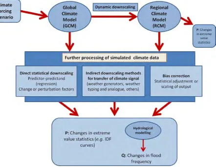
Assessment of climate change impacts on flood frequency due to projected changes in extreme precipitation requires a methodology comprising of a series of linked models and analyses (Figure 3.1). The basis for all methodologies is climate change projections from large-scale Global Climate Models (GCMs), which model coupled atmospheric-oceanic processes for historical and future periods. The GCM model runs are based on climate forcing scenarios representing various alternatives as to how society and technology will

develop through the 21st century (and in some cases beyond) and the impacts this will have

on greenhouse gas emissions and concentrations. Examples of climate forcing scenarios

include the IPCC SRES scenarios (e.g. Nakićenović et al., 2000) and the newer RCP

[image:24.595.97.540.274.616.2]

(Representative Concentration Pathways) scenarios (Meinshausen et al., 2011).

Figure 3.1 Relationships between various models and methodologies used to interpret

likely changes in extreme precipitation and flood frequency under a future climate.

Output from GCMs, typically having grid cell sizes of 100 – 250 km, is generally too coarse for direct analyses of flood generating processes, and further processing is required before likely changes can be assessed. This further processing takes the form of a dynamical downscaling using a regional climate model (RCM) and/or some form of statistical

(25)

alternative pathways between the GCM projections and a final analysis of likely changes in flood frequency, and most aspects of this process are currently under further development and refinement. Therefore, the diagram illustrated in Figure 3.1 should be taken as an attempt to sketch out a wide array of activity, rather than as a definitive distillation of a concrete set of methodologies.

A large proportion of the more recent analyses of likely changes in extremes are derived

from RCM simulations.RCMs are run for regional domains using a finer grid cell resolution

(e.g. 55; 25; 12.5 km) and input data from GCMs as boundary conditions. This process is

referred to as dynamical downscaling. During the past 10 years, two large EU FP6 projects have produced RCM simulations using higher resolution grids for modelling domains that

cover Europe. The PRUDENCE project (Christensen et al., 2007) focused on projections for

the end of the 21st century, whereas the ENSEMBLES project (van der Linden and Mitchell,

2009) produced transient simulations from the mid-twentieth century to 2100representing a

wide range of GCM/RCM combinations. There have also been several other regional, national and international projects that have focused on generating dynamically downscaled

RCM projections (e.g. EU FP6 CECILIA project,

(COordinated Regional climate Downscaling Experiment,

regional climate change scenarios globally. Work on regional climate modelling is continuing with a focus on higher grid resolution and improved representation of small-scale processes, such as convective precipitation. However, there are currently limitations associated with

computational issues and with process representation (e.g. Baker and Peter, 2008) such that

the next step is not simply a matter of running the currently available climate models at higher spatial and temporal resolutions.

In some analyses of climate change impacts on precipitation extremes in Europe, likely regional changes under a future climate have been interpreted directly from RCM outputs

(e.g. Kyselý and Beranová, 2009; Kyselý et al., 2011; Hadjinicolaou et al., 2011; Hanel and

Buishand, 2011). However, it is often necessary to undertake further processing of GCM or RCM output prior to analysing changes in flood generating processes. This is particularly the case for analyses of catchment-scale impacts based on hydrological modelling requiring a daily (or higher temporal resolution) precipitation time series; however, it is also relevant for local-scale interpretation of likely changes in extreme precipitation. For the purposes of summarising approaches used for this further processing, it is useful to make a distinction between 1) direct statistical downscaling methods which use climate model output to derive adjustments that are applied directly to or are conditioned by observed time series; 2) more indirect methods which use changes in climate variables as interpreted from climate models to drive methods such as weather generators or climate analogue interpretations; and 3) methods for statistical bias correction of model output which adjust the output relative to observations for further direct use in modelling and analyses. The third category does not necessarily involve a change in spatial or temporal scale, and so, is distinguished here from downscaling methods in which bias correction is often already implicitly included. It should be noted that as methods continue to be developed, distinctions between the three groups of methods illustrated in Figure 3.1 become increasingly diffuse.

Direct statistical downscaling has been a popular method for working with GCM output due to the explicit need for refinement of spatial and temporal scales between the climate model and the information required for hydrological impact assessment. The classical approach for statistical downscaling is the use of a regression-based relationship between predictors from the GCM (such as sea level pressure, temperature, geopotential heights and others) and local scale climate variables (such as precipitation and temperature). The use of this method

has been particularly facilitated by the SDSM software developed by Wilby et al. (2002),

although refinements of this general approach have also now been developed (e.g. see

(26)

also an example of direct statistical downscaling from GCM output to produce regional climate simulations (Enke et al., 2005).

The most widely-used approaches for statistical downscaling from both GCM and RCM

model output have, however, been the ‘delta change’ or ‘perturbation’ methods (e.g.

Reynard et al., 2001) due to their simplicity. In the most basic application of this technique,

estimates of monthly changes in average precipitation are derived by comparing monthly values from climate model output between a reference and a future period. These ‘change factors’ are then used to derive a time series of precipitation for the future by multiplication of the observed time series (for temperature an additive rather than a relative change is

ussually applied to the observed series).A considerable fraction of the studies which have

considered climate change impacts on flood frequency (Table 3.1) have used this simple

approach (e.g. Reynard et al., 2001; Prudhomme et al., 2003; Kay et al., 2006;

Kriaučiūnienė et al., 2008, Reynard et al., 2010; Veijalainen et al., 2010) or have combined

or compared it with other approaches (e.g. Lawrence and Haddeland, 2011; Sunyer et al.,

2012). The methodology has, however, been expanded to develop ‘quantile-perturbation’

factors for other statistics such as rainfall event intensities and frequencies (e.g. Boukhris

and Willems, 2008; Olsson et al., 2009; Willems and Vrac, 2011) and inclsion of changes in

precipitation variance (Sunyer et al., 2012), and this development is of particular relevance

for projecting changes in extreme precipitation and flood frequency. In addition, the

application of change factors for the probability of wet vs. dry days, is a considerable

improvement over change factors based on monthly changes in mean precipitation without such adjustment.

Indirect downscaling methods that have been applied to assess likely changes in extreme precipitation and flood frequency include, among others, the use of stochastic rainfall models or weather generators, the application of weather typing and resampling methods, and the use of climate analogues. When used for downscaling from climate models, stochastic

rainfall models (e.g. Semenov et al., 1998; Brissete et al., 2007; Burton et al., 2008) are set

up using probability distribution functions conditioned by outputs from the climate model, and these parameters are typically altered using ‘change factors’, such that the general

methodology has much in common with direct downscaling. The difference, however, lies in the use of a rainfall simulator as an intermediate step for generating precipitation time series used for further analyses. The approach is particularly useful, for example, for studies of

likely changes in subdaily precipitation intensities (e.g. Segond et al., 2007) if suitable

observed data are available for calibration of the rainfall simulator. Comparisons between different weather generators and with change factor methods indicate that certain weather generators are apparently more suitable for evaluating changes in extremes than simple

change factor methods (Sunyer et al., 2012), although other studies have indicated that

rainfall simulation methods may underestimate climate change impacts on extreme

precipitation (Arnbjerg-Nielsen, 2012). Weather typing (and related resampling) is also used

for downscaling precipitation (e.g. Enke et al., 2005; Boé et al., 2006; Vrac et al., 2007) and

is based on the concept of grouping days with synoptic similarity to define a finite set of weather types. Downscaling with this method takes the general form of identifying the

relevant weather type for each day simulated by the climate model based on e.g. simulated

pressure and temperature. The precipitation for that day is then selected from an observed precipitation series for a day having similar conditions. However, there are many variations

of this approach (e.g. resampling of Orlowsky et al., 2008). A general limitation of many

weather type approaches is that they do not allow for precipitation values which exceed those found in the observations. Alternatives, though, include relating future precipitation to

both weather type and to temperature (e.g. Willems and Vrac, 2011) and the use of

analogue data from other locations with observed precipitation series.

The first two sets of methodologies described above involve the use of quantities derived

from climate model output to either directly adjust an observed series (e.g. change factor

(27)

series from RCMs are also used more directly for analyses, for example, of precipitation statistics or as input to hydrological models. For local scale analyses of precipitation and for catchment-scale hydrological modelling, it is generally necessary to bias correct the climate model output prior to further analyses. There are several methods for achieving this

correction, such as a simple correction of the mean of the climate model output (e.g.

Graham et al., 2007), empirical adjustment methods that correct the mean and the standard

deviation (Engen-Skaugen, 2007; Leander and Buishand, 2007), distribution-based

corrections using gamma functions (e.g. Piani et al., 2010) or double-gamma functions

(Yang et al., 2010), and also bias corrections based on quantile-quantile plots (e.g. Déqué,

2007). The application of these techniques should also include a strategy for adjusting the number of rainy days, particularly if the precipitation data are to be used to analyse changes in flood frequency.

Analyses of changes in extreme precipitation are undertaken either directly on RCM output or on adjusted data. With respect to evaluating likely changes in flood hazard resulting from

extreme precipitation (e.g. urban flooding), the focus is often on changes in short-term

extreme precipitation statistics or on IDF (intensity-duration-frequency) relationships (e.g.

see review of Willems et al., 2012). In some recent cases, projections have been further

applied to assess their impact on urban drainage systems (e.g. Olsson et al., 2009; Willems

et al., 2010). For evaluating climate change impacts on the frequency of river flooding,

hydrological models are used to simulate discharge time series. Many of the hydrological models applied in the climate change studies reported in Table 3.1 are lumped and semi-distributed conceptual models such as HBV (Bergström, 1995; Sælthun, 1995), NAM

(Nielsen and Hansen, 1973), PDM (Moore, 2007), GR4J (Perrin et al., 2003), SWIM

(Krysanova et al., 1998), VHM (see overview in Taye et al., 2011), and WSFS

(Vehviläinen,1994). Distributed, grid-based models such as ASGi, (Becker and Braun,

1999), CLASSIC (Crooks et al., 2000; Reynard et al., 2001), G2G (Bell et al., 2007),

LARSIM (Ludwig and Bremicker, 2006), and MIKE SHE (Graham and Butts, 2006) have also been used in climate change impact analyses of flooding. In most cases, the grid-based distributed models include surface flow routing, such that climate change impact on flood runoff can, in principle, be estimated at each point in the model grid. For more detailed flood risk assessment studies hydrodynamic models have been applied, such as the MIKE 11

model (Havnø et al., 1995). In addition to gridded, distributed hydrological models, land

surface climate models and integrated hydrological and meteorological models, such as

CLSM (Koster et al., 2000; Ducharne et al., 2000) and SIM (Habets et al., 2008) have been

used for evaluating likely climate change impacts on flooding (Ducharne et al., 2010).

Figure 3.1 and the discussions in the preceding paragraphs show that there are numerous alternative approaches for assessing climate change impacts on flood frequency using climate model projections. The various alternative climate forcing scenarios, climate projections from available GCMs and RCMs, methods for statistical downscaling and bias correction, as well as alternative hydrological models can produce differing projections for the impact variable of interest. Consequently, a large proportion of climate change impact analyses now consider at least a number of climate projections to produce a distribution of outcomes, rather than relying on a single climate projection. This methodology is now commonly referred to as a type of ‘ensemble’ modelling approach and has been used in a

large number of the studies described in

Error! Reference source not found.

. However, in

(28)

3.2 Summary of country review reports

The reported studies on climate change projections of extreme precipitation and flood frequency are summarised in Table 3.1. The summary includes information about:

1. Study location: nationwide, regional, specific river basins or catchments

2. Climate change projections applied: GCMs, RCMs and analysed climate forcing scenarios

3. Bias correction and/or statistical downscaling method(s) applied

4. Hydrological modelling approach: type and name of hydrological model(s) applied and information on simulation approach

5. Variable considered, i.e. extreme precipitation (for given durations) or flood frequency 6. Summary of key findings, including projection horizon

7. References

A summary of the general findings and comparison with observed trends is given in Section 3.3.

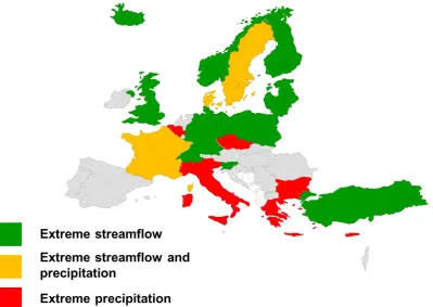
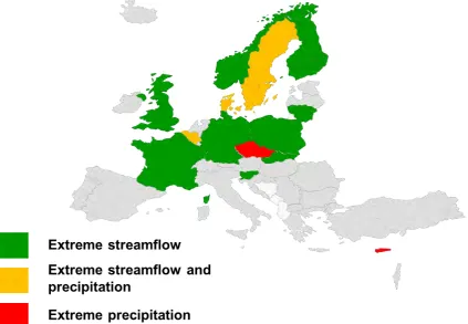
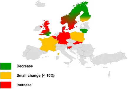
[image:28.595.82.506.327.620.2]

Climate change projections have been reported for 14 countries in Europe with results for extreme precipitation, extreme streamflow or both, see overview in Figure 3.2.

Figure 3.2 Overview of countries with reported studies on projection of extreme

(29)

[image:29.842.92.746.72.514.2]

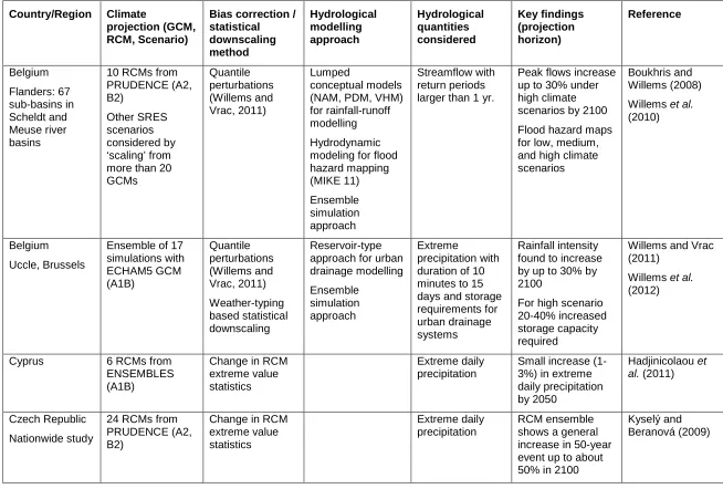
Table 3.1 Summary of country review reports on projections of precipitation extremes and floods under future climate change.

Country/Region Climate

projection (GCM, RCM, Scenario)

Bias correction / statistical downscaling method Hydrological modelling approach Hydrological quantities considered Key findings (projection horizon) Reference Belgium Flanders: 67 sub-basins in Scheldt and Meuse river basins

10 RCMs from PRUDENCE (A2, B2) Other SRES scenarios considered by ‘scaling’ from more than 20 GCMs Quantile perturbations (Willems and Vrac, 2011) Lumped conceptual models (NAM, PDM, VHM) for rainfall-runoff modelling

Hydrodynamic modeling for flood hazard mapping (MIKE 11) Ensemble simulation approach Streamflow with return periods larger than 1 yr.

Peak flows increase up to 30% under high climate scenarios by 2100

Flood hazard maps for low, medium, and high climate scenarios

Boukhris and Willems (2008)

Willems et al.

(2010)

Belgium

Uccle, Brussels

Ensemble of 17 simulations with ECHAM5 GCM (A1B) Quantile perturbations (Willems and Vrac, 2011) Weather-typing based statistical downscaling Reservoir-type approach for urban drainage modelling Ensemble simulation approach Extreme precipitation with duration of 10 minutes to 15 days and storage requirements for urban drainage systems

Rainfall intensity found to increase by up to 30% by 2100

For high scenario 20-40% increased storage capacity required

Willems and Vrac (2011)

Willems et al.

(2012)

Cyprus 6 RCMs from ENSEMBLES (A1B)

Change in RCM extreme value statistics

Extreme daily precipitation

Small increase (1-3%) in extreme daily precipitation by 2050

et

al. (2011)

Czech Republic

Nationwide study

24 RCMs from PRUDENCE (A2, B2)

RCM ensemble shows a general increase in 50-year event up to about 50% in 2100

(30)

European flood-frequency analysis in a changing environment Page 20 Czech Republic

Nationwide study

12 RCMs from ENSEMBLES (A1B)

Increase in 100-year event by about 23 % in 2100 (average of 12 RCMs)

Kysely et al.

(2011)

Czech Republic

Nationwide study

Regional non-stationary index-flood model (Hanel et al., 2009)

Extreme precipitation for durations

between 1 and 30 days

RCM ensemble shows a general increase in extreme precipitation by 2100, up to about 30% of 50-year daily precipitation Hanel and Buishand (2011) Denmark North-Eastern Sealand

4 RCMs from ENSEMBLES (A1B) Mean correction (delta change method) Mean and variance correction (Sunyer et al., 2012)

Three stochastic rainfall

generators: Markov Chain (Brisette et al., 2007); LARS (Semenov et al., 1998); RainSim (Burton et al., 2008). Distributed, physically-based hydrological model (MIKE SHE) Ensemble simulation approach Extreme daily precipitation Flood frequency Significant increase in daily precipitation extremes, up to a factor 2 for a 100-year event in 2100. Largest increases obtained with weather generator downscaling.

Significant increases in flood statistics, up to more than a factor 2 for a 100-year event for some catchments.

Sunyer et al.

(2010)

Sunyer et al.

(2012)

Denmark

Southern Jutland

Mean and variance correction (Sunyer et al., 2012) Weighted ensemble Semi-distributed, conceptual rainfall-runoff model (NAM)

MIKE 11 river model Extreme daily precipitation Flood frequency Extreme daily precipitation

increases about 9% in 2050 and 15% in 2100. Similar changes are seen in the extreme catchment runoff

Madsen et al.

(31)

European flood-frequency analysis in a changing environment Page 21 average changes

in mean and variance used for statistical downscaling statistics. Denmark Nationwide study HadAM3H/ HIRHAM4 RCM from PRUDENCE (A2)

Change in RCM extreme value statistics Stochastic rainfall generator Climate analogue Extreme precipitation for duration between 1 and 24 hours

Increases in extreme rainfall intensities by 10 – 50% within the next 100 years.

Arnbjerg-Nielsen (2012)

Finland

Nationwide study

15 GCMs and 5 RCMs from ENSEMBLES (A2, A1B, B1)

Delta change method Semi-distributed, conceptual rainfall-runoff model (WSFS) Ensemble simulation approach

Flood frequency 100-year floods decrease on average by 8–22% by 2100. Largest decrease in central Finland. Small increase in southern Finland. Increases in large central lakes.

Veijalainen et al.

(2010)

France

Seine and Somme catchments

8 GCMs (1 or 2 SRES scenarios each, 12

scenarios in total)

Dynamic

downscaling and bias correction of distribution (Déqué, 2007)

Weather typing (Boé et al., 2006) Perturbation method

(Ducharne et al., 2007) 5 hydrological models, representing both lumped, conceptual and distributed, physically-based models (MODCOU, SIM, CLSM, EROS/GARDENIA, GR4J) Ensemble simulation approach

Flood frequency 10-year flood magnitudes do not change

significantly; ±10% in most cases (2045-2065 and 2080-2100)

Ducharne et al.

(32)

European flood-frequency analysis in a changing environment Page 22 Germany Bavaria and Baden-Württemberg ECHAM4/REMO RCM (B2)

WettReg (Enke et al., 2005)

STAR (Orlowsky

et al., 2008)

Two distributed hydrological models (LARSIM and ASGi) Ensemble simulation approach

Flood frequency 15% increase in 100-year flood in Bavaria and up to 75% in 2-year flood and up to 25% increase in 100-year flood in Baden-Württemberg (2021-2050).

KLIWA (2011)

Hennegriff et al.

(2006)

Germany

Saxony -Anhalt

ECHAM5/REMO RCM (A2, A1B, B1)

WettReg (Enke et al., 2005)

Semi-distributed, conceptual rainfall-runoff model (SWIM) Ensemble simulation approach; WettReg generated 20 realizations of each scenario

Flood frequency Significant increases in flood frequency. Up to 60% increase in 50-year flood (2011– 2040, 2041–2070 and 2071–2100)

Hattermann et al.

(2011) Lithuania Nemunas catchment ECHAM5 and HadCM3 GCMs (A2, A1B, B1)

Regression relationships between large and local scale monthly means

Delta change method

Lumped,

conceptual rainfall-runoff model (HBV)

Ensemble simulation approach

Flood frequency Significant

decreases in spring flood magnitude, between 25-60% (2011-2040, 2041-2070 and 2071-2100)

Kriaučiūnienė et al. (2008)

Meilutytė-

Barauskiene et al.

(2010)

Norway

Nationwide study

4 RCMs from PRUDENCE (A2, B2) Delta change method Empirical adjustment method (Engen-Skaugen, 2007) Lumped, conceptual rainfall-runoff model (HBV)

Ensemble simulation approach Uncertainty in hydrological parameters

Flood frequency Western Norway has the largest percentage increases in flood magnitude (up to 60% increase in 200-year flood by 2100). Catchments in inland regions are generally

(33)

included expected to have

reduced flood magnitudes.

Poland

Wełna and Orla

catchments

Quantile mapping Lumped,

Flood frequency In western Poland, the simulation results for different RCM/GCMs indicate different directions of change or lack of statistically

significant changes.

Kaczmarek (2003)

Romanowicz et al.

(2011)

Slovakia

Hron catchment

3 GCMs Calculation of changes in short-term extreme precipitation totals based on projected changes in monthly temperature and specific humidity Lumped, conceptual rainfall-runoff model developed at Slovak University of Technology Maximum discharge for selected extreme precipitation events Increases in discharge up to 80% in 2030 and up to 140% in 2075.

Hlavčová et al.

(2007)

Slovenia

Nationwide study

Details not given Details not given Lumped,

Flood frequency In the Alpine and hilly catchments increase in flood peaks of about 30%. In karstic areas increases of about 10%.

Kobold (2009)

Sweden

Kalmar

2 RCA3 RCMs (A2 and B2)

Scaling of distribution of rainfall intensities 30-min extreme precipitation Extreme intensities will increase by 20– 60% in 2100

Olsson et al.

(2009)

Sweden

Stockholm

3 RCA3 RCMs (A2,B2 and A1B)

Stochastic downscaling scheme Extreme precipitation for durations between 30 min

5–10% increase in short-duration extreme intensities in the period 2011–

Olsson et al.

(34)

European flood-frequency analysis in a changing environment Page 24 and 24 hours 2040 and a 10–

20% increase in the period 2071–2100

Sweden

Nationwide study

16 RCMs Distribution based scaling (Yang et al., 2010)

Lumped,

Flood frequency In the central part of the country, floods tend to decrease, mainly due to decreasing snowmelt floods in spring, while rain-fed floods in the south show the opposite tendency.

Bergström et al.

(2012)

UK

River Severn and Thames

HadCM2 GCM Delta change method

Distributed rainfall-runoff model (CLASSIC)

Flood frequency 50-year flood in the Severn and

Thames increase by 20% and 16%, respectively by 2050.

Reynard et al.

(2001)

UK

5 catchments

7 GCMs (A1, A2, B1, B2)

GCMs perturbed using a climate sensitivity based rescaling approach Delta change method Lumped, conceptual rainfall-runoff model (PDM) Ensemble simulation approach

Flood frequency Increase in flood magnitude for most scenarios by 2050.

Prudhomme et al.

(2003) UK 15 catchments HadRM3H RCM (A2) Delta change method Lumped, conceptual rainfall-runoff model (PDM)

Flood frequency Decrease in flood magnitude in south and east England, 50% increase in 50-year flood in north and west UK by 2100.

Kay et al. (2006)

UK

154 catchments

16 GCMs and 11 versions of HadRM3 RCM (A1B) Delta change method Lumped, conceptual (PDM) and distributed (CLASSIC)

rainfall-Flood frequency The median of the ensemble show few catchments with changes in flood

Reynard et al.

(35)

European flood-frequency analysis in a changing environment Page 25 runoff models

frequency above 20% by 2010. However, considering the large uncertainty in the ensemble the 20% change factor can no longer be considered precautionary.

UK

Nationwide study

HadRM3 RCM (A1B)

Ensemble of three perturbed

parameter simulations

No statistical downscaling of RCM

Lumped,

conceptual (PDM) and distributed (G2G) rainfall-runoff models

Flood frequency Upward trend in flood risk nationally

Kay and Jones (2012)

A2, A1B, B1, B2: IPCC SRES scenarios (Nakićenović et al., 2000)

ECHAM4, ECHAM5: GCM developed by Max Planck Institute for Meteorology, Germany