A Determination of the Lambda Parameter from Full Lattice QCD

Determination of the Lambda parameter from full lattice QCD

M. Go¨ckeler,1,2R. Horsley,3A. C. Irving,4D. Pleiter,5P. E. L. Rakow,4G. Schierholz,5,6and H. Stu¨ben7 (QCDSF-UKQCD Collaboration)

1_{Institut fu¨r Theoretische Physik, Universita¨t Leipzig, 04109 Leipzig, Germany} 2_{Institut fu¨r Theoretische Physik, Universita¨t Regensburg, 93040 Regensburg, Germany}

3_{School of Physics, University of Edinburgh, Edinburgh EH9 3JZ, United Kingdom}

4_{Theoretical Physics Division, Department of Mathematical Sciences, University of Liverpool, Liverpool L69 3BX, United Kingdom} 5_{John von Neumann-Institut fu¨r Computing NIC, Deutsches Elektronen-Synchrotron DESY, 15738 Zeuthen, Germany}

6_{Deutsches Elektronen-Synchrotron DESY, 22603 Hamburg, Germany} 7_{Konrad-Zuse-Zentrum fu¨r Informationstechnik Berlin, 14195 Berlin, Germany}

(Received 25 February 2005; revised manuscript received 12 December 2005; published 23 January 2006)

We present a determination of the QCD parameterin the quenched approximation (nf 0) and for

two flavors (nf2) of light dynamical quarks. The calculations are performed on the lattice usingOa

improved Wilson fermions and include taking the continuum limit. We findMS

nf0259119MeVand MS

nf22611726MeV, usingr00:467 fmto set the scale. Extrapolating our results to five flavors, we obtain for the running coupling constant at the mass of theZbosonMS

s mZ 0:11212.

DOI:10.1103/PhysRevD.73.014513 PACS numbers: 11.15.Ha, 12.38.Gc

I. INTRODUCTION

The parameteris one of the fundamental quantities of QCD. It sets the scale for the running coupling constant

s, and it is the only parameter of the theory in the

chiral limit. Usually is defined by writingsas an

expansion in inverse powers of ln2=2. For such a relationship to remain valid for all values of , must change as flavor thresholds are crossed:!_nf, where

n_findicates the effective number of light (with respect to the scale) quarks.

A lattice calculation ofrequires an accurate determi-nation of a reference scale, the introduction of an appro-priate nonperturbatively defined coupling, which can be computed accurately on the lattice over a sufficiently wide range of energies, as well as a reliable extrapolation to the chiral and continuum limits. Finally, and equally impor-tantly, one needs to know the relation of the coupling to

MS

s , the quantity of final interest, accurately to a few

percent. This program has been achieved for the pure gauge theory [1,2]. In full QCD calculations with Wilson fermions the amount of lattice data was barely enough to enable a reliable chiral and continuum extrapolation [2,3]. Recent calculations with staggered fermions cover a wider range of lattice spacings and quark masses [4]. However, staggered fermions are not without their own problems.

We determine in the MS scheme from the force parameterr0[5] and the ‘‘boosted’’ couplingg䊐. The latter

is obtained from the average plaquette. The advantage of this method is that both quantities are known to high precision. As in our previous work [2,3], we shall use here nonperturbatively Oa improved Wilson (clover) fermions. Definitions of the action are standard (see, for

example, Appendix D of [6]). The lattice calculations will be done for nf 2flavors of dynamical quarks. In

addi-tion, we will update our quenched results.

Since our first attempt [2,3] the amount of lattice data with dynamical quarks has greatly increased [7]. That is to say, at our previous couplings5:20, 5.25 and 5.29 we have increased the statistics and done additional simula-tions at smaller quark masses. Furthermore, we have gen-erated dynamical gauge field configurations at 5:40 for three different quark masses. At eachvalue we now have data at three to four quark masses at our disposal, and the smallest lattice spacing that we have reached in our simulations isa0:07 fm. This allows us to improve on, and disentangle, the chiral and continuum extrapolations. In the quenched case the force parameter r₀=a is now known up to6:92[8].

The paper is organized as follows. In Sec. II we present a general discussion about the function, including Pade´ approximations, and the running coupling constant. Also given are results in theMSscheme. In Sec. III we set up the lattice formalism and discuss what coefficients are known. Various possibilities for converting to theMSscheme are given, which will indicate the magnitude of systematic errors. In Sec. IV results are given for r₀MS _{for both}

quenched (n_f0) and unquenched n_f2 fermions. These results are then extrapolated to nf3 flavors of

dynamical quarks in Sec. V. This is done by matching the static force at the scaler0. In Sec. VI we convert our results

to physical units and, after matchingstonf5flavors,

II. THE QCD COUPLING AND THEFUNCTION

The ‘‘running’’ of the QCD coupling constant as the scale changes is controlled by thefunction,

@g_SM

@logM

S_g

SM (1)

with

Sg_S b0g3_Sb1g5_SbS2g7SbS3g9S ; (2)

renormalization having introduced a scaleMtogether with a schemeS. The first two coefficients are scheme indepen-dent and are given for theSU3color gauge group as

b0

1

42

112

3nf

; b1

1

44

10238

3 nf

:

(3)

Integrating Eq. (1) gives

S

M F

S_g

SM (4)

with

FS_g

S exp

1

2b0g2S

b₀g2

S b1=2b20

exp

ZgS

0 d

₁

S

1

b03

b1 b2 0 ; (5)

where S, the integration constant, is the fundamental scheme dependent QCD parameter. The integral in Eq. (5) may be performed numerically or to low orders analytically. For example, to 3 loops we have

S

M exp

1

2b₀g2

S

b0g2_Sb1=2b

2 0

1 A

S

2b0 g2 S pS A

1 B

S

2b₀g 2 S pS B ; (6) where

ASb₁ b2

14b0bS2

q

; BSb₁ b2

14b0bS2

q

;

(7)

and

pS_A b1

4b2₀ b2

12b0bS2

4b2 0

b2

14b0bS2

q ;

pS B

b1

4b2 0

b

2

12b0bS2

4b2₀ b2₁4b0bS2

q :

(8)

Results are usually given in theMS scheme, with the scaleMbeing replaced by, and thus

MS

F

MS_g

MS: (9)

In this scheme the next two function coefficients are known [9–11]:

bMS

2

1

46

₂₈₅₇

2 5033

18 nf 325 54 n 2 f ; bMS 3 1

48

_{149 753}

6 35643

_{1 078 361}

162 6508

27 3

n_{f 50 065} 162 6472

81 3

n2 f 1093 729 n 3 f : (10)

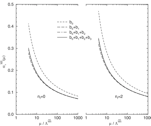
The running couplingMSs g2_MS=4is plotted in

Fig. 1 forn_f0, 2 by solving Eq. (5) numerically, using only the first coefficient (1-loop), the first and second coefficients (2-loop) etc. of the function. The figure shows an apparently rapidly convergent series (cf. the 3-to 4-loop result), certainly in the range we will be inter-ested in, =MS_{20. The main difference between the} n_f0 and n_f2 results is that MS

s jnf2 rises more steeply as a function of=MS_{, asb}

0jnf2< b0jnf0. A knowledge of thefunction to 4 loops is the excep-tion rather than the rule. In many schemes it is known only to 3 loops. To improve the convergence of thefunction, we may attempt to use a Pade´ approximation by writing Eq. (2) as

1 10 100 1000

µ / ΛMS 0.0 0.1 0.2 0.3 0.4 0.5 αs MS ( µ ) b0

b₀+b₁

b₀+b₁+b₂

b₀+b₁+b₂+b₃

1 10 100 1000

µ / ΛMS

n_f=0 n_f=2

FIG. 1. MS

s versus =MS fornf0 (left picture) and nf2(right picture), using successively more and more

S₁₌₁g_S b0g

3

S b1 b0bS2

b1 g

5

S

1bS2 b1g

2

S

; (11)

which on expanding is arranged to give the first three coefficients of Eq. (2) and estimates the next coefficient

bS₃ as

bS

3

bS₂2 b1

: (12)

It is again possible to give an analytic result forFS using

S₁₌₁. We find

S

M exp

1

2b₀g2

S

_b

0g2_S

1 b1 b0

bS 2 b1g

2

S

b1=2b20

: (13)

At least for theMSscheme this appears to work reasonably well. Equation (12) givesbMS

3 3:2210

5 _and1:67

105_{for quenched and unquenched fermions, respectively,}

to be compared with the true values from Eq. (10) of 4:70105 _{and 2:7310}5_{. In [3] we have shown a}

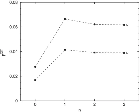
figure of the various Pade´ approximations to the func-tion. In Fig. 2 we show the value ofFMSg_MSatg2

MS2

versus the function coefficient number for both quenched and unquenched fermions. Also shown are the results using the1=1Pade´ approximations. It is seen that these numbers lie extremely close to the 4-loopfunction results. As Pade´ approximations give some estimation of the effect of higher orderfunction coefficients, we shall thus prefer these later in our determination of the parameter.

III. LATTICE METHODS

On the lattice we also have a coupling constantg₀aand corresponding function with coefficients bLAT

i and

pa-rameterLAT_{, where}

aLAT _FLAT_g

0a: (14)

To evaluateFLAT, we need to know thebLAT_i s. They can be found by expandingg_MS as a power series ing0 as

1

g2 MS

1

g2 0a

2b₀lnatLAT 1

2b1lnatLAT2 g02a 2b0b1ln2a

2bMS

2 b1tLAT1 lnatLAT3 g40a :

(15)

To have consistency between Eqs. (9) and (14) we need

tLAT

1 2b0ln

MS

LAT; (16)

and

bLAT₂ bMS₂ b1tLAT1 b0tLAT2 ;

bLAT

3 bMS3 2bMS2 tLAT1 b1tLAT1 22b0tLAT3 ;

(17)

where bLAT

i are the lattice function coefficients, as in

Eq. (2). So the transformation between the two schemes is given by the tLAT

i (which define the transformation), and

the renormalization group dictates how the scale running occurs (in this case thelnaterms). A knowledge of (the 1-loop) tLAT

1 determines the relationship between the

parameters in the two schemes, while also knowing (the 2-loop) tLAT

2 means that the 3-loopfunction coefficient bLAT

2 can be found.

At present, what we know is [2,12 –17]

tLAT

1 0:468 201 3nf0:006 696 00:005 046 7csw

0:029 843 5c2

swamq0:027 283 7

0:022 350 3c_sw0:007 066 7c2

sw Oamq2; tLAT

2 0:055 667 5nf0:002 6000:000 155csw

0:012 834c2sw0:000 474c3sw0:000 104c4sw

Oamq: (18)

HeretLAT

1 has been calculated including theamqterms (mq

being the bare quark mass), while tLAT

2 is known only for am_q0, and tLAT

3 is unknown, which means that from

Eq. (17) bLAT₂ is known but notbLAT₃ . For general csw the

connection betweeng2 MSandg

2

0is only defined up to terms

of Oa, but on the improvement trajectory csw

1Og2

0 it is possible to arrange it to be Oa2 if the amq terms are included in thetLATi s.

0 1 2 3

n 0

0.02 0.04 0.06 0.08

F

MS

FIG. 2. FMS_g

MSfor g

2

MS 2 versus function coefficient

numbern. Thenf0values are filled circles, while thenf2

values are filled squares. The 1=1 Pade´ approximations are given as open symbols.

Thus, the conversion from the lattice coupling to theMS

coupling [Eqs. (15) and (18)] can also be written with mass independenttLAT

i s, if we redefineg20 by replacing it byg~20,

where

~

g2₀ g2₀1bgamq; bgb 0

g nfg20Og40:

(19)

So, puttingcsw1Og20into Eqs. (15) and (18) means

that tLAT

1 is replaced by tLAT1 nfamqb 0

g , which gives bg00:012 00. This value agrees with the number

re-ported in [18].

Thus, in this mass independent scheme (i.e. a scheme where the renormalization conditions are imposed for zero quark mass) there appears to be little difference in extrap-olating to the chiral limit using constant6=g2

0, rather

than constant~6=g~₀2_{. So, rather than using Eq. (18) at}

finiteamq, we shall first extrapolate our plaquette andr0=a

data to the chiral limit and then determine MS_{. Before}

attempting this, we shall discuss some improvements to help improve the convergence of the power series (15).

As it is well known that lattice perturbative expansions are poorly convergent, we have used a boosted coupling constant

g2 䊐

g2₀a

u4 0

(20)

to help the series (15), or equivalently (2) forLAT_g 0,

converge faster. HereP u4

0 hTrU䊐i=3is the average

plaquette. In perturbation theory we write

1

g2 䊐

1

g2 0

p1p2g02Og40 (21)

with [19,20]

p₁1 3;

p20:033 911 0nf0:001 8460:000 053 9csw

0:001 590c2

sw (22)

for massless clover fermions.

To improve the convergence of the series further, we reexpress it in terms of the tadpole improved coefficient

c䊐swcswu30: (23)

ChangingtLAT

i to t䊐i first replacestiLAT bytLATi pi, and

secondly using c䊐_sw simply replaces every c_sw by c䊐_sw in

tLAT

1 , but the change in t䊐2 is more complicated as the

coefficients ofc䊐swchange int䊐2.

This gives fort䊐_i t䊐_i c䊐_swin the chiral limit

t䊐₁ 0:134 868 0n_f0:006 696 00:005 046 7c䊐_sw

0:029 843 5c䊐sw2;

t䊐₂ 0:021 756 5n_f0:000 7530:001 053c䊐_sw

0:000 498c䊐sw20:000 474c䊐sw3

0:000 104c䊐sw4: (24)

As we have here a 2-loop result, we can see how well tadpole improvement improves the series convergence. The coefficient of n_f in t䊐₂ is considerably smaller than the corresponding coefficient in tLAT₂ . For example, using the values at 5:40given in the next section, we find that the magnitude of the coefficient is reduced by 2 orders of magnitude (from 0:0438to0:0003).

What this tadpole improvement represents is taking a path fromg20tog2g2_䊐, keepingc䊐swfixed. Later we

shall consider other trajectories from 0 tog2

䊐. If we had all orders of the theory, the result would depend only on the end point. But with a finite series the trajectory will matter. This will help us estimate systematic errors from unknown higher order terms.

Thus, in conclusion we have

a䊐 F䊐g_䊐a; (25)

MS

F

MS_g

MS; (26)

together with the conversion formula

1

g2 MS

1

g2_䊐a2b0lnat

䊐 1

2b₁lnat䊐₂g2

䊐a (27)

with

t䊐₁ 2b₀ln

MS

䊐 (28)

and

b䊐₂ bMS₂ b1t䊐1 b0t䊐2: (29)

We shall now discuss various strategies to determine MS_.

A. Method I

This method was used in our previous papers [2,3,21], with the difference that now we first extrapolate to the chiral limit. For each value we first compute t䊐_i from Eq. (24). Then from Eq. (27) we convertg_䊐tog_MSat some appropriate scale , and using the force scale r0, we

r0MS r0FMSgMS: (30)

Finally, we extrapolate to the continuum limit,a!0. Note thatt䊐_i will depend on the coupling becausec䊐swdoes.

We must determine the scale. A good choice to help

Eq. (27) converge rapidly is to take theO1coefficient to vanish, which is achieved by choosing [13]

1

aexp

_t䊐

1

2b0

: (31)

Thus, we used

1

g2 MS

1

g2 䊐a

_b

1 b0

t䊐₁ t䊐₂

g2

䊐a Og4䊐 (32)

to findg2

MS, which was then substituted into Eq. (30).

B. Method II

Alternatively, we can first determineb䊐₂ from Eq. (29) and then determine r₀䊐 via Eq. (25). After computing this, we convert tor₀MS_using

r0MSr0䊐exp

_t䊐

1

2b0

; (33)

and then take the continuum limit. Again, note thatb䊐₂ will depend on the coupling, becausec䊐_swdoes.

This method is equivalent to choosing a scale, as in

method I, such thatg_MS g䊐a. In this caseallthe coefficient terms of Eq. (27) vanish. The scale that achieves this is

1

aexp

_t䊐

1

2b0

_F䊐_g

䊐a

FMS_g

䊐a

: (34)

Indeed, substituting into Eq. (26) then gives Eq. (33) again. The scale is close to , as can be seen by expanding Eq. (34) to 3 loops. From Eq. (6) we have

1

aexp

_t䊐

1

2b₀

1A䊐

2b0g

2 䊐p䊐A

1AMS

2b0g

2 䊐p

MS A

1B䊐 2b0g

2 䊐p䊐B

1BMS

2b0g

2 䊐p

MS B

1b1t䊐1 b0t䊐2

2b2₀ g 2

䊐

> ; (35)

for the couplings used here.

C. Method III

Another possibility, and theoretically the most sound, is to varyc䊐_sw along the improvement path asg2

䊐 increases. This will give genuinely constant function coefficients (i.e. independent of the coupling). As the 1-loop expansion forc䊐swis known along this path,

c䊐sw1c䊐0g2䊐 ; (36)

with c䊐₀ c034p1 and c0 0:26591 [22], then

ex-panding Eq. (24) gives

b䊐₂ bMS

2 b1t䊐1jc䊐sw1b0t 䊐

2jc䊐sw1b0c 䊐 0

@t䊐₁ @c䊐_sw

c䊐sw1

0:000 824 1: (37)

This result may also be derived from Eq. (27) by first setting a1 _{(for simplicity) and then taking @=@}

of this equation. This leads to

2

g3 MS

MSg_MS

2

g3_䊐 @t䊐₁ @c䊐sw

@c䊐sw @g_䊐2t

䊐 2g䊐

Og3 䊐

䊐g_䊐; (38)

which upon expanding out also gives Eq. (37).

So, having determinedb䊐₂ in Eq. (29), the method is as for method II: first determiner₀䊐using Eq. (25) and then convert tor₀MS_{using Eq. (33).}

D. Methods IIP and IIIP

To further improve our calculations, and to reduce the systematic error, we consider here the effect of Pade´ im-proving thefunction, as given in Eqs. (11) and (13). We restrict ourselves to methods II and III, and we call the Pade´ improved results IIP and IIIP, respectively.

IV. RESULTS

A. Quenched results

In the quenched case (nf0) we do not have any of the

additional chiral limit extrapolation complications alluded to in the previous section, or a c_swterm. This means that there is no difference between method II and method III, so the procedure is straightforward. In Table I we give the parameters used. For r0 we use, for consistency,

exclu-sively the values given in [8], which includes previous results from [23]. The one exception is 6:0, where we have used the interpolation formula [8] for r0=a. Our

plaquette values are determined at their givenvalues. In Table I we also give the results for r0MS from

methods I, II and IIP. We first see that the results for

r0MS are almost indistinguishable between methods I,

II and IIP. Method IIP lies just below method I (and indeed is almost identical to it).

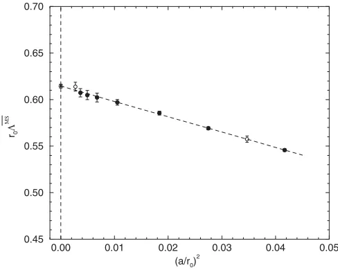
We now consider the continuum limit of our results. In Fig. 3 we plot the results for r₀MS _{against a=r}

02 for

method IIP. The differences between the results of the various methods are small. As one expects that Pade´ im-provement gives a better answer, we shall concentrate on IIP. The smallest a value is not included in the fit, as it appears to deviate a little, but including it would not have changed the extrapolated value much. We also have not included6:0in the fit, asr0=ais only known from an

interpolation formula. But as can be seen from the figure,

including it has no effect on the result. Also, the two coarsest a values have not been included in the fit, as they show significant nonlinear effects in a2_{. These two}

points are not shown in the plot, as they lie far to the right. Figure 3 clearly shows a linear extrapolation over a wide range of lattice spacings,a1_{2–6:5 GeV, giving a value}

for method IIP of

r₀MS

0 r0MSjnf0 0:61425: (39)

Here the first error is statistical, and the second systematic error is estimated by the spread in the results between methods I, II and IIP. That the systematic error is small is

an indication of the convergence of results from the differ-ent methods. The result (39) agrees with our earlier value [2].

B. Unquenchednf 2results

We now turn to unquenchedn_f2fermions. In Table II we show the,andcswparameters used in the

simula-tions, together with the measured r₀=a, the plaquette val-uesPand the pseudoscalar massesam_PS. As discussed in Sec. III, we shall first determiner₀MS _{in the chiral limit}

and then perform the continuum extrapolation. We must thus first find the zero quark mass results from Table II. We shall make a chiral extrapolation inamq, defined here by

amq

1 2

₁

1

_c

: (40)

We estimate _c from partially quenched pion data. The results have been given in [7] and are tabulated in the second column of Table III. For the reader’s convenience we give the spatial box sizesLand the pseudoscalar masses in physical units for our unquenched simulations in Table IV usingr0 0:467 fmto set the scale.

In Fig. 4 we show the results for the plaquette as a function of the quark mass. The data appear to be rather linear in the quark massamq, in particular for the higher

values. The mass dependence of Phas been computed in perturbation theory toOg4

0and found to be well

parame-terized by a second order polynomial in amq for amq<

0:25[19]. We thus use

Pd0d1amqd2amq2; (41)

withd0,d1andd2depending on, to extrapolate our data

to the chiral limit. The results are given in the fourth column of Table III.

TABLE I. The quenchedr0MSvalues for methods I, II and IIP (i.e. using the Pade´ improved

function䊐₁₌₁) together with the force parameterr0=a[8] (the number at6:0is from the interpolation formula given there) and the plaquette P. The continuum extrapolated values together with the statistical errors are given in the bottom row. Numbers initalicsare not used in the fits.

r0=a P r0MS I r0MS II r0MS IIP 5.70 2.922(09) 0.549 195(25) 0.4888(15) 0.4950(15) 0.4888(15)

5.80 3.673(05) 0.567 651(21) 0.5142(07) 0.5200(07) 0.5140(07)

5.95 4.898(12) 0.588 006(20) 0.5461(13) 0.5514(14) 0.5457(13) 6.00 5.368(33) 0.593 679(08) 0.5579(34) 0.5631(35) 0.5575(34)

6.07 6.033(17) 0.601 099(18) 0.5696(16) 0.5746(16) 0.5692(16) 6.20 7.380(26) 0.613 633(02) 0.5861(21) 0.5907(21) 0.5855(21) 6.40 9.740(50) 0.630 633(04) 0.5976(31) 0.6018(31) 0.5970(31) 6.57 12.18(10) 0.643 524(15) 0.6029(48) 0.6067(48) 0.6022(48) 6.69 14.20(12) 0.651 936(15) 0.6055(50) 0.6091(51) 0.6049(50) 6.81 16.54(12) 0.659 877(13) 0.6080(46) 0.6113(46) 0.6073(46) 6.92 19.13(15) 0.666 721(12) 0.6145(47) 0.6177(47) 0.6139(47)

1 1 1 0.6152(21) 0.6189(21) 0.6145(20)

0.00 0.01 0.02 0.03 0.04 0.05 (a/r0)

2 0.45

0.50 0.55 0.60 0.65 0.70

r0

Λ

MS

To test for systematic errors, we have performed linear fits inam_qin the regionam_q0:04. The chiral limit value ofPwas found to change by a small amount between0:2w at5:20and0:01wat5:40. Adding a cubic term to Eq. (41) leads to a formula with four fit parameters. Only at 5:20 and 5:29 are sufficiently many data points available to perform a four-parameter fit. It yields at the chiral limit P0:538 593950 for 5:20 and

P0:549 652293 for 5:29 corresponding to changes well below 1w. Thus we are confident that our chiral limit values of the plaquette are reliable.

In Fig. 5 we show the results for r0=a as a function

of amq. Writing P6=g2_䊐a, and using the

1-loop expressions 1=g2

䊐a 2b0ln1=a䊐 and

2b0lnMS=䊐 t䊐1, with t䊐1amq being given in [2],

we obtain in perturbation theory

lnr0

a e0e1amqe2amq

2_{; (42)}

where e₀, e₁ and e₂ depend on . In addition, due to spontaneous chiral symmetry breaking and cutoff effects, the force parameterr₀receives contributions not accounted for by lattice perturbation theory, which can be well fitted by a linear term inm_q[25]. We perform a global fit to our data, taking e₀ to be a linear polynomial in , in accor-dance with the 1-loop result, and e₁ ande₂ to be second

TABLE IV. The length Lof the spatial box and the pseudo-scalar mass in physical units for our unquenched simulations. The scale has been set usingr00:467 fm.

V L(fm) mPS(GeV)

5.20 0.134 2 163_{32 1.83 1.007(17)} 5.20 0.135 0 163_{32 1.57 0.833(08)} 5.20 0.135 5 163_{32 1.48 0.619(07)} 5.20 0.135 65 163_{32 1.42 0.548(12)} 5.20 0.135 8 163_{32 1.40 0.468(18)}

5.25 0.134 6 163_{32 1.58 0.987(11)} 5.25 0.135 2 16332 1.45 0.830(09) 5.25 0.135 75 243_{48 2.03 0.597(05)}

5.29 0.134 0 163_{32 1.55 1.173(20)} 5.29 0.135 0 163_{32 1.43 0.929(13)} 5.29 0.135 5 243_{48 2.01 0.769(09)} 5.29 0.135 9 243_{48 1.91 0.594(10)}

5.40 0.135 0 243_{48 1.84 1.037(11)} 5.40 0.135 6 243_{48 1.76 0.842(07)} 5.40 0.136 1 243_{48 1.67 0.626(06)} TABLE II. The unquenched,andcswvalues and the volumeV, together with the measured

force parameter r0=a and plaquette P. Also given are the pseudoscalar meson massesmPS,

though they do not enter the calculation. We have reanalyzed our r0=a values, taking autocorrelations properly into account, which gave larger error bars than previously reported [24]. The lattice spacingaranges from 0.07 to 0.11 fm. The number of trajectories varies from

O3500on the 243_{48 lattices to O8000on the 16}3_{32 lattices, except for 5:29,} 0:1359, where we have accumulatedO2000trajectories so far.

V csw r0=a P amPS

5.20 0.134 2 163_{32 2.0171 4.077(70) 0.528 994(58) 0.5847(12)} 5.20 0.135 0 163_{32 2.0171 4.754(45) 0.533 670(40) 0.4148(13)} 5.20 0.135 5 163_{32 2.0171 5.041(53) 0.536 250(30) 0.2907(15)} 5.20 0.135 65 163_{32 2.0171 5.250(75) 0.537 070(100) 0.2470(40)} 5.20 0.135 8 163_{32 2.0171 5.320(95) 0.537 670(30) 0.2080(70)}

5.25 0.134 6 163_{32 1.9603 4.737(50) 0.538 770(41) 0.4932(10)} 5.25 0.135 2 16332 1.9603 5.138(55) 0.541 150(30) 0.3821(13) 5.25 0.135 75 243_{48 1.9603 5.532(40) 0.543 135(15) 0.2556(06)}

5.29 0.134 0 163_{32 1.9192 4.813(82) 0.542 400(50) 0.5767(11)} 5.29 0.135 0 163_{32 1.9192 5.227(75) 0.545 520(29) 0.4206(09)} 5.29 0.135 5 243_{48 1.9192 5.566(64) 0.547 094(23) 0.3269(07)} 5.29 0.135 9 243_{48 1.9192 5.880(100) 0.548 286(57) 0.2392(09)}

5.40 0.135 0 243_{48 1.8228 6.092(67) 0.559 000(19) 0.4030(04)} 5.40 0.135 6 243_{48 1.8228 6.381(53) 0.560 246(10) 0.3123(07)} 5.40 0.136 1 243_{48 1.8228 6.714(64) 0.561 281(08) 0.2208(07)}

TABLE III. The critical values for (i.e. c) and the chiral

limit values forr0=aandPfor the fourvalues used here.

c r0=a P

5.20 0.136 008(15) 5.455(96) 0.538 608(49) 5.25 0.136 250(07) 5.885(79) 0.544 780(89) 5.29 0.136 410(09) 6.254(99) 0.549 877(109) 5.40 0.136 690(22) 7.390(260) 0.562 499(46)

order polynomials in. This ansatz was also used in [7]. The results of the fits in the chiral limit are given in the third column of Table III.

Linear fits, i.e. fits with e₂ 0, in the region am_q

0:04lead to chiral limit values ofr0=a which differ from

those in Table III by less than the statistical error. Adding ane₃am_q3 _{term introduces another three parameters and}

gives rather large errors in the results. Within these errors they agree however with those obtained from the fit func-tion (42). We take this as evidence in favor of our extrapo-lation and shall henceforth use the numbers given in Table III.

In Table V we give our results forr₀MS_{for methods I,}

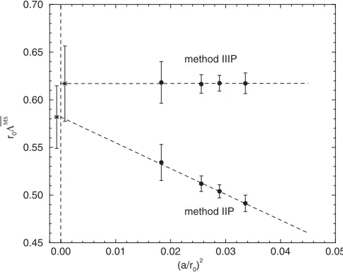
II, IIP, III and IIIP. Again, as the results for method I are very similar to method II, we shall not discuss method I further here. In Fig. 6 we plot r₀MS _{against a=r}

02 for

methods IIP and IIIP, together with a linear extrapolation to the continuum limit. Though we cannot reach such smalla

values as for the quenched case, ther0MSdata do seem to

lie on straight lines. We find a linear behavior at least over the region a1_{2–3 GeV. This seems to be well inside}

the linear region of Fig. 3.

For methods IIP (and II) the results lie roughly parallel to the quenched results, while for methods IIIP (and III) they are flatter and higher. However, in the continuum limit they agree within error bars. Ideally, the result should not depend on the choice of trajectory. The way this should work, as mentioned before, is that although the coefficients

t䊐_i will be different depending on the path one might choose, the sum

1

g2 䊐a

t䊐₁ t䊐₂g2_䊐a (43)

should not. However, at the order to which we have the series this is not yet so. The difference between methods II and III is that we have replacedc䊐swby its 1-loop expansion.

Returning to Fig. 6, the fact that the results from methods II, IIP are almost parallel to the quenched results suggests that in methods II, IIP the Oa2 _{effects come}

from the same source as in the quenched case, which must be the gluon action. For methods III, IIIP the slope is much smaller so there must have been a fortuitous cancellation betweena2 _{effects from the gluon and fermion terms.}

0 0.02 0.04 0.06 0.08

amq

4 5 6 7 8

r0

/a

FIG. 5. The force parameter r0=a plotted against amq. The

same notation as in Fig. 4 is used.

0 0.02 0.04 0.06 0.08

am_q 0.52

0.53 0.54 0.55 0.56 0.57

P

FIG. 4. The plaquette P (filled symbols) plotted against the bare quark massamqfor5:20(lower curve) until5:40

(upper curve). The fits use Eq. (41), giving the extrapolated values in the chiral limit (open symbols).

TABLE V. The values forr0MSfor methods I, II, IIP, III, IIIP described in Sec. III for the four

values used here.

r0MSI r0MS II r0MSIIP r0MSIII r0MS IIIP 5.20 0.5183(91) 0.5304(94) 0.4913(87) 0.6459(114) 0.6173(109) 5.25 0.5210(71) 0.5415(73) 0.5040(68) 0.6450(87) 0.6174(83) 5.29 0.5372(85) 0.5482(87) 0.5120(81) 0.6433(102) 0.6165(98) 5.40 0.5577(198) 0.5676(201) 0.5343(189) 0.6431(228) 0.6182(219)

One expects that Pade´ improvement gives a better an-swer, so the P results are more trustworthy. Previous expe-rience suggests that the procedure in IIP of using tadpole improvedcsw works fairly well. For example, c in [26]

and the renormalization constant Z for v_2b in [6] agree within a few percent with the nonperturbative values. However, method IIIP is a more consistent approach. Furthermore, the results from method IIIP appear to be insensitive to the particular form of the continuum extrapo-lation. We therefore take these numbers as our best estimate.

From the linear extrapolation of method IIIP to the continuum limit we thus quote

r0MS2 r0MSjnf2 0:6174021; (44)

where the first error is statistical and the second systematic. The latter error is estimated by the spread in the results between methods III and IIIP. Compared to our previous result [2], the value (44) has increased by10%, but still lies within the error bars.

V. EXTRAPOLATION TOnf 3FLAVORS

At high energy scales we can see thatMSmakes some fairly large jumps as we pass through the heavy quark mass thresholds and change the effective number of flavors. From [27] we can see that the reason for these large jumps is the fact thatm_q=MS_{is large. We want to argue here that}

the situation with light quarks,mq&MS, is rather

differ-ent, and that in this case we do not expect to see any dramatic dependence ofMS _onn

f.

We will determine then_f 3flavorparameter from matching the static force at the scaler0.

A. One-loop matching

To make clear what is involved in matching, we will go through the 1-loop calculation in some detail.

At the 1-loop level the static potential between funda-mental charges is given by

Vr 4

3

g2 MS

4r

1g

2 MS

162

22

lnrE

31 66

4

3nf

lnr_E5

6

(45)

for massless sea quarks (see, for example, [28]). We can work out the forcefrat distancerby differentiating this to give

4r2_fr 4

3g

2 MS

1g

2 MS

162

22

lnr_E35

66

4

3nf

lnrE

1 6 : (46)

If we now change the flavor number from 2 to 0, or from 2 to 3, while keeping the force at distancerconstant, we get

33 ln MS 0 MS 2 4 lnMS

2 rE

1 6

;

336ln

MS 3 MS 2 2 lnMS

2 rE

1 6

:

(47)

We can eliminate rfrom these equations, leaving us with the simple equation

MS 3 MS 2 MS 2 MS 0

11=18

; (48)

which can be used to estimate MS

3 from thenf0and nf2results.

B. Higher loops

To repeat this matching calculation with more loops, we follow [8] and define a force-scale couplinggqq by

4r2_fr 4

3g2qqr: (49)

From Eq. (46) we can read off

tqq₁ 1

42

22 E 35 66 4

3nf

E 1 6 : (50)

We can find tqq₂ by calculating the force from the 2-loop expression ofVrreported in [29,30]:

0.00 0.01 0.02 0.03 0.04 0.05 (a/r₀)2

0.45 0.50 0.55 0.60 0.65 0.70 r0 Λ MS method IIP method IIIP

FIG. 6. The unquenched r0MS _{points (filled circles) versus} a=r02, together with a linear extrapolation to the continuum limit for methods IIP and IIIP. Stars represent the extrapolated values.

tqq₂ 1 44

₁₁₀₇

2 204E 229

3

29

4

4₆₆ 3

nf

3

553

3 76E 44

3

2₅₂ 3

4

27n

2

f122

; (51)

which gives us enough information to calculate the 3-loop

function forg_qqr[cf. Eq. (17)]. There would be com-plications in going to the next order, because it is known that terms of the type4

slnswill enter the series for the

potential [31].

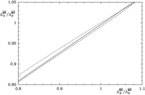
We are now ready to see how MS _{depends on flavor}

number, if we make the value offr independent ofn_f

(the number of massless quark flavors) at some particularr

value. Implicitly, we assumerr₀. Iffris independent ofn_f, theng_qqris independent ofn_f too. We can com-pare theqq schemes by using

rqq₀ Fqqgqqr; nf0;

rqq₂ Fqqgqqr; nf2;

rqq₃ Fqqgqqr; nf3:

(52)

We can take ratios of these equations to cancelrand find equations forratios. Theseqqschemeratios can then be converted intoMSby usingtq₁qfrom Eq. (50). This gives us a way of making a parametric plot ofratios by varying

gqq and calculating all three s from gqq. In Fig. 7 we

show the plot.

The results clearly have to be treated with some caution, becauser₀is a fairly large number. So it is not clear how much we can learn from perturbative results at the scaler₀. It is therefore quite surprising that the different orders of perturbation theory agree so well in Fig. 7. Furthermore, we have assumed in this section thatr0ms1, so that the

strange quark can reasonably be treated as massless. Both

these difficulties could be decreased by using a smaller distance [and thus a smaller value for r2_{fr] to set our}

scale.

C. Result forn_f 3

From our quenched and unquenchednf2results, (39)

and (44), we obtain MS

2 =MS0 1:005. If we insert this

number into the 3-loop matching curve shown in Fig. 7, we find MS

3 =MS2 0:999. Using this ratio and Eq. (44) we

obtain by extrapolation fornf3quark flavors

r₀MS

3 r0MSjnf30:6162919: (53)

We have not attempted to estimate the systematic error induced by the matching procedure.

VI. COMPARISON WITH PHENOMENOLOGY

In this section we shall make a comparison with other lattice and phenomenological results. For this we first need to set the force scaler0 in terms of a physical unit.

A popular (but somewhat arbitrary) choice is r0

0:5 fm, which is useful when making comparisons with other lattice results. Another choice is to use the nucleon mass, or some other hadron observable, to determine the physical value of r0. However, this is only possible after

extrapolating the observable to the physical pion mass. Encouraged by our comparison of nucleon mass data in different volumes with chiral perturbation theory [24,32], we have used the extrapolation procedure described in [24] as fit 1 to recent nucleon masses obtained by the CP-PACS and JLQCD Collaborations along with updated masses from the QCDSF-UKQCD Collaboration. This means that we have fixed gA1:267, f92:4 MeV, c2

3:2 GeV1 _{and c}

3 3:4 GeV1 in the fit function

[Eq. (16) in Ref. [24]]. Varying the assumed physical value ofr0one can make the fit curve pass through the physical

point, which happens forr00:467 fm. This number has

been confirmed recently in a lattice calculation off[33],

givingr0 0:47525fm. A similar result forr0was also

quoted in [34] taking as input level splittings in the spectrum. Therefore we shall use the value r0

0:467 fm in the following, but consider r₀0:5 fm as well in order to estimate the systematic error caused by the uncertainty in setting the scale. Note that previously [2] we had assumedr₀ 0:5 fm.

For the quenched case we obtain withr₀ 0:467 fm

MS

0 25912MeV;

and for the unquenched case we find

MS

2 261179MeV; MS3 260128MeV: FIG. 7. The ratioMS

The corresponding numbers forr₀0:5 fmare

MS₀ 24212 MeV; MS₂ 244168 MeV;

MS

3 243117 MeV:

Adding the effect of the scale uncertainty to the system-atic error we quote as our final results

MS₀ 259119 MeV; (54)

MS

2 2611726MeV; (55)

MS

3 2601225MeV: (56)

In Fig. 8 we show our results for MS _{together with}

recent experimental values from [35,36]. It appears that the lattice results extrapolate smoothly to the experimental values atnf4[35] andnf5[36]. However, ournf

3result lies 2 standard deviations below the corresponding phenomenological value (open triangle). (The reader should be aware that the sometimes called experimental numbers imply a good deal of modeling and, thus, should be regarded as phenomenological numbers.)

In order to compare s from various experiments and

theory, it must be evolved to a common scale. For

conve-nience this is taken to be the mass of the Z boson, m_Z. Having computedMS_forn

f3flavors, we may use the

4-loop expansion ofsand the 3-loop matching condition

at the quark thresholds [27,37] to determine MS_n

f5mZ. We take the charm and bottom thresholds to be at 1.5 and 4.5 GeV, respectively. Furthermore, we choose the charm and bottom quark masses to bemMS

c mc 1:5 GeVand mMS_b mb 4:5 GeV, respectively. Varying the charm and

bottom quark masses within reasonable limits has a negli-gible effect on the final result. We then obtain

MS

nf5mZ 0:11212: (57)

This is to be compared with the world average value [36]

MSs mZ 0:118227.

In Fig. 9 we compare our result forMSs mZwith other

lattice results and experiment. We find agreement with previous lattice calculations using Wilson fermions. It occurs that the Wilson results lie systematically below the mean experimental value. On the other hand, calcula-tions using staggered fermions (albeit from the same group) show a better agreement with experiment. Our result for r0MS2 agrees also with that of the ALPHA

Collaboration [38], which does not quote a number for

FIG. 9. Comparison ofMS

s mZfrom this work (solid circle)

with other lattice results [40 – 42,2,43,4,44,21] (from top to bottom). The circles are from Wilson fermions and the squares from staggered fermions. The dashed line indicates the mean phenomenological value [36].

FIG. 8. Values ofMS_{versus number of quark flavorsn} f. The

filled circles are ournf0, 2 results, and the open circle is our

extrapolated value. The inner error bars give the statistical errors, while the outer error bars give the total errors. The square is from a 3-loop analysis of the nonsinglet structure functions [35]. The triangles are taken from [36]. The open triangles are evaluated using the 4-loop expansion ofs and 3-loop matching at the

quark thresholds. The entries atnf3 and 4 have been

dis-placed horizontally.

MS

s mZ. Our result for MSs mZ lies 2 standard

devia-tions below the phenomenological value.

VII. CONCLUSIONS

Because of substantial improvements of the perform-ance of our hybrid Monte Carlo algorithm [39], we were able to extend our dynamical simulations to smaller quark masses and to larger values of . Our smallest lattice spacing now is a0:07 fm. This enabled us to perform a chiral and continuum extrapolation of the lattice data. Because the calculation involves a perturbative conversion from the lattice coupling constant to the (mass indepen-dent)MSconstant, it was important to first extrapolate the lattice data to the chiral limit. We have discussed basically two approaches of converting the lattice coupling constant to theMS one. They differed mainly in how the nonper-turbative improvement (clover) term was incorporated in the perturbative expansion. It was reassuring to see that both methods led to the same result in the continuum limit. This indicates once more that a reliable extrapolation to the continuum limit is very important.

We could also improve on our quenched result, because data at smaller lattice spacings became available.

There are several sources of systematic error in our calculation. The main error comes from setting the scale, followed by the continuum extrapolation. As better dy-namical data become available, the uncertainty in setting the scale will be gradually reduced. Simulations at smaller lattice spacings will become possible with the next gen-eration of computers, which should facilitate the extrapo-lation to the continuum limit.

ACKNOWLEDGMENTS

We would like to thank Antonios Athenodorou and Haris Panagopoulos for checking the numbers in Eq. (22). The numerical calculations have been performed on the Hitachi SR8000 at LRZ (Munich), on the Cray T3E at EPCC (Edinburgh) [45], on the Cray T3E at NIC (Ju¨lich) and ZIB (Berlin), as well as on the APE1000 and Quadrics at DESY (Zeuthen). We thank all institutions. This work has been supported in part by the EU Integrated Infrastructure Initiative Hadron Physics (I3HP) under Contract No. RII3-CT-2004-506078 and by the DFG under Contract No. FOR 465 (Forschergruppe Gitter-Hadronen-Pha¨nomenologie).

[1] S. Capitani, M. Lu¨scher, R. Sommer, and H. Wittig, Nucl. Phys.B544, 669 (1999).

[2] S. Booth, M. Go¨ckeler, R. Horsley, A. C. Irving, B. Joo´, S. Pickles, D. Pleiter, P. E. L. Rakow, G. Schierholz, Z. Sroczynski, and H. Stu¨ben, Phys. Lett. B 519, 229 (2001).

[3] S. Booth, M. Go¨ckeler, R. Horsley, A. C. Irving, B. Joo´, S. Pickles, D. Pleiter, P. E. L. Rakow, G. Schierholz, Z. Sroczynski, and H. Stu¨ben, Nucl. Phys. B, Proc. Suppl.106, 308 (2002).

[4] C. T. H. Davies, E. Follana, A. Gray, G. P. Lepage, Q. Mason, M. Nobes, J. Shigemitsu, H. D. Trottier, M. Wingate, C. Aubin, C. Bernard, T. Burch, C. DeTar, S. Gottlieb, E. B. Gregory, U. M. Heller, J. E. Hetrick, J. Osborn, R. Sugar, D. Toussaint, M. Di Pierro, A. El-Khadra, A. S. Kronfeld, P. B. Mackenzie, D. Menscher, and J. Simone, Phys. Rev. Lett. 92, 022001 (2004).

[5] R. Sommer, Nucl. Phys.B411, 839 (1994).

[6] M. Go¨ckeler, R. Horsley, D. Pleiter, P. E. L. Rakow, and G. Schierholz, Phys. Rev. D71, 114511 (2005).

[7] M. Go¨ckeler, R. Horsley, A. C. Irving, D. Pleiter, P. E. L. Rakow, G. Schierholz, and H. Stu¨ben, hep-ph/0409312. [8] S. Necco and R. Sommer, Nucl. Phys. B622, 328

(2002).

[9] O. V. Tarasov, A. A. Vladimirov, and A. Yu. Zharkov, Phys. Lett.93B, 429 (1980).

[10] S. A. Larin and J. A. M. Vermaseren, Phys. Lett. B 303, 334 (1993).

[11] T. van Ritbergen, J. A. M. Vermaseren, and S. A. Larin, Phys. Lett. B400, 379 (1997).

[12] M. Lu¨scher and P. Weisz, Phys. Lett. B 349, 165 (1995).

[13] M. Lu¨scher, hep-lat/9802029.

[14] B. Alle´s, A. Feo, and H. Panagopoulos, Phys. Lett. B426, 361 (1998).

[15] S. Sint (private communication), quoted in A. Bode, P. Weisz, and U. Wolff, Nucl. Phys.B576, 517 (2000). [16] L. Marcantonio, P. Boyle, C. T. H. Davies, J. Hein, and

J. Shigemitsu, Nucl. Phys. B, Proc. Suppl.94, 363 (2001). [17] A. Bode and H. Panagopoulos, Nucl. Phys. B625, 198

(2002).

[18] M. Lu¨scher, S. Sint, R. Sommer, and P. Weisz, Nucl. Phys.

B478, 365 (1996).

[19] G. S. Bali and P. Boyle, hep-lat/0210033.

[20] A. Athenodorou, H. Panagopoulos, and A. Tsapalis, Nucl. Phys. B, Proc. Suppl.140, 794 (2005).

[21] M. Go¨ckeler, R. Horsley, A. C. Irving, D. Pleiter, P. E. L. Rakow, G. Schierholz, and H. Stu¨ben, Nucl. Phys. B, Proc. Suppl.140, 228 (2005).

[22] M. Lu¨scher and P. Weisz, Nucl. Phys. B479, 429 (1996).

[23] M. Guagnelli, R. Sommer, and H. Wittig, Nucl. Phys.

B535, 389 (1998).

[25] R. Sommer, S. Aoki, M. Della Morte, R. Hoffmann, T. Kaneko, F. Knechtli, J. Rolf, I. Wetzorke, and U. Wolff, Nucl. Phys. B, Proc. Suppl.129, 405 (2004).

[26] M. Go¨ckeler, R. Horsley, H. Perlt, P. Rakow, G. Schierholz, A. Schiller, and P. Stephenson, Phys. Rev. D

57, 5562 (1998).

[27] K. G. Chetyrkin, B. A. Kniehl, and M. Steinhauser, Phys. Rev. Lett.79, 2184 (1997).

[28] I. Montvay and G. Mu¨nster,Quantum Fields on a Lattice

(Cambridge University Press, Cambridge, 1994). [29] Y. Schro¨der, Phys. Lett. B447, 321 (1999). [30] M. Peter, Nucl. Phys.B501, 471 (1997).

[31] T. Appelquist, M. Dine, and I. J. Muzinich, Phys. Rev. D

17, 2074 (1978).

[32] M. Procura, T. R. Hemmert, and W. Weise, Phys. Rev. D

69, 034505 (2004).

[33] M. Go¨ckeler, R. Horsley, D. Pleiter, P. E. L. Rakow, G. Schierholz, W. Schroers, H. Stu¨ben, and J. M. Zanotti, Proc. Sci. LAT2005 (2005) 063. See, e.g., http://pos. sissa.it/POSreaders.html

[34] C. Aubin, C. Bernard, C. DeTar, Steven A. Gottlieb, E. B. Gregory, U. M. Heller, J. E. Hetrick, J. Osborn, R. Sugar, and D. Toussaint, Phys. Rev. D70, 094505 (2004). [35] J. Blu¨mlein, H. Bo¨ttcher, and A. Guffanti, Nucl. Phys. B,

Proc. Suppl.135, 152 (2004).

[36] S. Bethke, Nucl. Phys. B, Proc. Suppl. 121, 74 (2003);

135, 345 (2004).

[37] K. G. Chetyrkin, B. A. Kniehl, and M. Steinhauser, Nucl. Phys.B510, 61 (1998); K. G. Chetyrkin, J. H. Ku¨hn, and M. Steinhauser, Comput. Phys. Commun.133, 43 (2000).

[38] M. Della Morte, R. Frezzotti, J. Heitger, J. Rolf, R. Sommer, and U. Wolff, Nucl. Phys. B713, 378 (2005).

[39] T. Bakeyev, M. Go¨ckeler, R. Horsley, D. Pleiter, P. E. L. Rakow, G. Schierholz, and H. Stu¨ben, Phys. Lett. B580, 197 (2004).

[40] S. Aoki, M. Fukugita, S. Hashimoto, N. Ishizuka, H. Mino, M. Okawa, T. Onogi, and A. Ukawa, Phys. Rev. Lett.74, 22 (1995).

[41] C. T. H. Davies, K. Hornbostel, G. P. Lepage, P. McCallum, J. Shigemitsu, and J. Sloan, Phys. Rev. D

56, 2755 (1997).

[42] A. Spitz, H. Hoeber, N. Eicker, S. Gu¨sken, Th. Lippert, K. Schilling, T. Struckmann, P. Ueberholz, and J. Viehoff, Phys. Rev. D60, 074502 (1999).

[43] P. Boucaud, J. P. Leroy, H. Moutarde, J. Micheli, O. Pe`ne, J. Rodrı´guez-Quintero, and C. Roiesnel, J. High Energy Phys. 01 (2002) 046.

[44] Q. Masonet al., talk at Lattice, 2004; Q. Mason, H. D. Trottier, C. T. H. Davies, K. Foley, and G. P. Lepage, Nucl. Phys. B, Proc. Suppl. 140, 713 (2005); Q. Mason, H. D. Trottier, C. T. H. Davies, K. Foley, A. Gray, G. P. Lepage, M. Nobes, and J. Shigemitsu, Phys. Rev. Lett.95, 052002 (2005).

[45] C. R. Allton, S. P. Booth, K. C. Bowler, J. Garden, A. Hart, D. Hepburn, A. C. Irving, B. Joo´, R. D. Kenway, C. M. Maynard, C. McNeile, C. Michael, S. M. Pickles, J. C. Sexton, K. J. Sharkey, Z. Sroczynski, M. Talevi, M. Teper, and H. Wittig, Phys. Rev. D65, 054502 (2002).