This is a repository copy of A Review of Methods for Estimating Origin-Destination Trip Matrices Using Link Counts..
White Rose Research Online URL for this paper: http://eprints.whiterose.ac.uk/2069/
Monograph:
Timms, P.M. (2001) A Review of Methods for Estimating Origin-Destination Trip Matrices Using Link Counts. Working Paper. Institute of Transport Studies, University of Leeds , Leeds, UK.
Working Paper 556
[email protected] https://eprints.whiterose.ac.uk/
Reuse
See Attached
Takedown
If you consider content in White Rose Research Online to be in breach of UK law, please notify us by
White Rose Research Online
http://eprints.whiterose.ac.uk/
Institute of Transport Studies University of Leeds
This is an ITS Working Paper produced and published by the University of Leeds. ITS Working Papers are intended to provide information and encourage discussion on a topic in advance of formal publication. They represent only the views of the authors, and do not necessarily reflect the views or approval of the sponsors.
White Rose Repository URL for this paper:
http://eprints.whiterose.ac.uk/2069/
Published paper
Paul Timms (2001) A Review of Methods for Estimating Origin-Destination Trip
March
2001
A REVIEW OF METHODS FOR ESTIMATING
ORIGIN-DESTINATION TRIP MATRICES USING LINK COUNTS
1.1.1
Paul Timms
INSTITUTE FOR TRANSPORT STUDIES DOCUMENT CONTROL INFORMATION
Title A review of Methods for Estimating Origin-Destination Trip Matrices Using Link Counts
Author(s) Paul Timms
Editor
Reference Number WP556
Version Number 1.0
Date March 2001
Distribution Public
Availability unrestricted
File K\common\office\workpap\wp556
Authorised O.M.J. Carsten
Signature
© Institute for Transport Studies, University of Leeds
Abstract
The paper concludes by making recommendations, both philosophical and methodological, concerning both practical applications and further research.
3. Introduction
The main purpose of this paper is the creation of a philosophical structure for classifying methods which estimate origin-destination trip matrices using link counts. The first question that might be asked about such an aim is 'why bother?'. Two immediate responses can be made:
• From ad-hoc personal experience, there is often a large amount of confusion when matrix estimation methods are used in typical practical urban transportation planning studies. This is particularly the case when planners have had experience of different types of method. Frequently, this confusion concerns two specific issues: the distinction between a priori and observed information; and the distinction between old (observed) data and present-day (observed) data. Different methods deal with these issues in different ways, according to the underlying philosophical approach of the method. If the distinctions between these underlying approaches are not clearly demarcated (for example, if the methods are solely categorised according to their mathematical form) the confusion is liable to increase.
• With the help of increased availability of 'PC computer power' there is an increasing trend towards more complex transportation modelling. In particular, highly complex strategic multimodal transnational models are already being produced which estimate (network) traffic flows under a range of differing future scenarios (see e.g. Williams et al (1998)). It is argued here that matrix estimation techniques using link counts are important for helping to calibrate these models. Due to the complexity of the models, it is important that any calibration technique used is fully understood by its user. It can be argued that whilst a lack of understanding might not have too serious an effect in a typical urban modelling application, it is liable to have a much greater effect in a strategic application.
The paper is organised as follows. Section 2 introduces some of the relevant concepts informally by considering some questions arising from an 'outline' specification of the problem. Section 3 lists some practical applications for methods of matrix estimation using link counts. Some of these applications have already made use of such methods; the other applications are likely to do so in the future. As an example of the latter, consideration is given to 'prescriptive strategic applications', which might become widespread within the next decade. Section 4 presents the philosophical framework itself. Section 5 shows how different philosophical approaches lead to differing methods, by making a review of papers on the subject covering the last 30 years. Section 6 summarises the general conclusions that result from the paper, and in particular lists recommendations for further research and recommendations for action by transport planners (when using matrix estimation techniques).
4.1 Outline specification of the problem
A useful starting point for discussion of the issues in this paper is to consider a (loosely defined) outline specification of the problem as follows:
Problem 1
Consider a geographical area which is divided into n zones {ZI : i=1,...n}. Define
the flow of trips from zone i to zone j, over a given time period, to be Tij. Then the
problem is to make an optimal estimate of the matrix {Tij}, by combining prior
information on {Tij} with information resulting from a set of link flow observations
{ : a=1,...m} made on a set of links A over the same time period. It is assumed
that is an observation on the flow F $
Fa $
Fa a along link a , where
a ij
ij ija
F = ∑T p ∀a∈A (2.1)
and where pija is the proportion of trips from i to j that use link a.
Equation (2.1) captures the straightforward concept that link flows, origin-destination flows and assignment proportions are all related to each other. However, a number of issues immediately arise from this outline specification. The discussion of these issues leads directly both to the development of tighter definitions of the problem, as well as to the consideration of different types of philosophical approaches that can be used for finding solutions. These issues can be listed under the following headings (and are discussed fully in Sections (2.2) to (2.6) respectively):
• temporal
• assignment
• spatial
• prior information
• role of the method-user
4.2 Temporal issues
Probably the most striking questions about Problem 1 arise from the fact that there are no references to time in it: (2.2.1) to (2.2.3) contain three significant temporal questions.
4.2.1 Within-period static states
A first question that might be asked is about Problem 1 is:
Problem 1 implicitly assumes a static state of affairs within the period being considered. Thus, for example, if eqn (2.1) refers to a peak period, there is an underlying assumption that the traffic pattern is essentially stable throughout this peak. It follows immediately that 'off-peak' traffic cannot affect conditions in the peak (at either its beginning or end). This assumption is made in many practical applications. However, as soon as we want to take into account that change may occur during the modelled period, or that traffic in an earlier time period has an effect on traffic in a later time period, we need to make an explicit representation of within-period dynamics.
A typical method for considering within-period dynamics involves the introduction of the concept of time slices to Problem 1. Thus the matrix {Tij} is extended to the matrix
{Tijs} in one of the alternative following ways:
1. {Tijs} represents the flow leaving zones {i} in time slice s
2. {Tijs} represents the flow arriving at zones {j} in time slice s
3. {Tijs} represents the flow arriving at count points {a} in time slice s
Assuming Definition 1 for {Tijs}, Problem 2 can be formulated as follows:
Problem 2
An optimal estimate is required of {Tijs}, and is reached by combining prior
information on {Tijs} with information resulting from a set of link flow
observations { } made over a set of time slices {t}. It is assumed that is an observation on the flow F
$
Fat F$at
t
a along link a , where
(2.2)
a t
ij s ijs ijsa
t
F = ∑ ∑T p
and where
is the proportion of T
pijsat ijs that passes along link a in time slice t
4.2.2 One-off periods or means
A second temporal question that might be asked is:
(ii) Do the flows in eqns (2.1) or (2.2) refer to a one-off period in history, or do they represent a mean over a number of 'similar' periods?
A simple interpretation of eqns 2.1 and 2.2 is that they refer to a particular period in history such as 'between 13.00 and 14.00 on Friday 21st May'. This is actually how the equations are used in real-time control strategies (albeit typically with rather shorter time slices than one hour). However, this interpretation is not likely to be useful to transport planners, who are usually interested in 'average' situations rather than one-off situations. Planners will generally require that eqns (2.1) and (2.2)
represent mean flows over a set of 'homogenous' time periods, such as 'weekday am peak periods'.
In the case of the single 'one-off' interpretation of eqns (2.1) and (2.2) it cannot be guaranteed that Fa = , or that , because of measurement errors, such as
vehicles being counted inaccurately. This difficulty also applies if eqns (2.1) and (2.2) refer to mean flows. However, there is a further difficulty in this case in that { } and { } will only provide estimates of mean flows (calculated from a sample), unless of course the link counts are made on a 'permanent' basis. There will thus be further uncertainty that F
$
Fa Fa F t
a t
= $
$
Fa F$at
a = F$a , or that Fa F . t
a t
= $
4.2.3 Long term trends
A final temporal question that might be asked is:
(iii) Are there any long term trends (in terms of growth or decline) underlying the traffic system?
Separate to the issues of within-day statics, eqns (2.1) and (2.2) represent a system that has no long term trends in growth or decline; i.e. they represent a long term static
system. There are two main methods for representing long term change:
• The traffic system can be represented as going through a number of discrete jumps (for example one jump per year). In between jumps the system can be represented as in a (long term) static state, and it can be assumed that there will be a separate set of eqns (2.1) or (2.2) for each such static period. This approach can be termed a revolutionary model, since it implicitly assumes that there is a revolution in transport behaviour (including demand) associated with each jump.
• Alternatively, there could be an explicit representation of the traffic system going through long term continuous change: this model could be termed an evolutionary
4.3 Assignment issues
In the use of eqns (2.1) and (2.2), assumptions must be made about assignment (i.e. the factors {pija} and { }). In the within-period static case, these assumptions
concern spatial issues (i.e. the routes taken by interzonal flows): for the within-period dynamic case, the assumptions concern both spatial and temporal issues.
pijsat
In some applications, the assignment assumptions are dictated automatically by the characteristics of the network. Where this is not the case, though, there is a need to employ an assignment model which can estimate {pija} and { }. An important
(implicit) assumption made throughout Section 2.2 was that assignment was 'fixed'. However, each temporal issue discussed in (2.2) has an equivalent assignment variation issue:
pijsat
• assignment is likely to vary on a within-period basis;
• there is likely to be variation in assignment on a day-to-day basis, even if the transport system were to be in a long term static state;
• there is likely to be underlying long term change in assignment.
4.4 Spatial issues
Two spatial issues arise from eqns (2.1) and (2.2), and from the method for constructing an assignment model:
(i) How are intrazonal trips treated?
(ii) Are all 'real-life' links represented in the network?
If intrazonal trips are ignored, eqns (2.1) and (2.2) will both be internally inconsistent, since there are potentially 'extra' intrazonal trips on each link.
On the other hand, if any 'real-life' links (carrying interzonal traffic) are neglected in the network representation, eqns (2.1) and (2.2) will both be internally inconsistent, since the modelled links will have an exaggerated level of flow on them.
In most urban applications, issues (i) and (ii) are assumed to 'cancel each other out'; the justification for this being that the errors involved are small. However, in interurban applications (with large zones and large levels of intrazonal traffic as a percentage of all traffic), no such simplifying assumption can be made.
4.5 Prior information
Problem 1 refers to prior information on {Tij} being used in combination with link
counts in order to estimate trip matrices. There are two essentially different sources for such prior information:
(i) Prior information could come from direct observations made on elements of {Tij}, collected 'at the same time' as the observations { }. Given the temporal
difficulties discussed in (2.2), there are inevitably some difficulties about a precise definition of 'at the same time'. However, an informal understanding (representing the same level of looseness found in eqn (2.1)) should be clear.
$ Fa
(ii) Prior information could come from 'elsewhere', such as from a demand model or from an 'old' matrix.
In general prior information of type (i) can be handled by standard statistical techniques whereas prior information of type (ii) is more problematic methodologically. As a result, this paper will put more emphasis on issues related to type (ii) information.
4.6 Role of the method-user
A central theme of this paper concerns how the method-user deals with the 'trip matrix estimation from link counts' problem when faced with the questions mentioned in Sections 2.2 to 2.5 above. A formal definition of the positions that the method-user can take are given in Section 4 below. This section covers some of the issues informally.
It should be clear from above that there is a trade-off between, on the one hand, specifying the problem in a comprehensively precise fashion and, on the other hand, representing the problem more loosely. The attraction of the former approach is due directly to its rigour and the resulting confidence that the method-user can have when presenting any results. The advantages of the looser approach are that it is likelier to be easier to understand (and hence to explain) and likely to be less demanding in terms of data needs.
The question that immediately arises concerns how worthwhile it is to try to make precise the specification of the problem. Since a large amount of current research is tied up with exactly this activity (as will be discussed in Section 5 below), this aim should not be belittled. On the other hand, it is important to point out that none of the methods for calculating OD matrices from link counts referred to in Section 5 could be said to be completely precise (although, not surprisingly, some are defined more clearly than others).
decide upon an approach that best meets all the (potentially conflicting) demands upon the model. A first intention of this paper is to try (in Section 4) to provide a philosophical context to help understand how decisions on choice of approach might be made by the method-user; this context is then used to provide a classification of method-types in Section 5. Firstly, though, in Section 3, some information is given upon the type of applications for which planners use the methods described in this paper.
5. Overview of application areas
5.1 Introduction
Arguably, it is urban (city-wide) planning applications that have provided the most usage for methods to estimate trip matrices by using link counts. The stereotypical application here is of a 'standard' planning study where an assignment software package is used to predict the effects of a number of potentially implementable transport schemes. Examples of currently well-used software packages are EMME2, SATURN, TRIPS and TransCAD.
The schemes tested by these packages can be classified as either traffic management schemes (for which the trip matrix is usually considered to be constant) or schemes which alter travel demand. In either case, it is essential to have available an up-to-date 'do-nothing' trip matrix. The trip matrices used in such applications will typically be:
• matrices of vehicle trips, differentiated by vehicle type as appropriate: such matrices are used for assessing (fixed demand) traffic management schemes
• matrices of person trips, for use in assessing schemes which alter demand (typically between private and public transport)
Link count methods are particularly useful for estimating matrices of vehicle trips, since counts on vehicle link flows are collected regularly and are typically reasonably accurate. Furthermore, link count methods can also be used to estimate public transport passenger trip matrices, thus enabling total (car user and public transport user) trip matrices to be estimated. However, link counts of public transport passengers are typically more problematic than link counts of vehicles. For example, link counts of bus passengers are often made by observers who, standing at the roadside, need to make fast estimates of total bus occupancy. Such estimates are liable to high degrees of measurement error, especially if bunching of buses occurs at peak times.
From these basic applications, three particular further applications can be identified:
• applications on small networks (sometimes only one junction)
• strategic interurban multimodal applications
• the absorption of link count approaches in 'general frameworks to estimate trip matrices' which use a variety of different types of data.
These four applications are discussed in (3.2) to (3.5) respectively.
5.2 Applications on small networks
Small networks are here considered to be either single junction networks or single motorway networks. The trip matrices to be estimated concern entry-to-exit movements for the junction or motorway respectively. An example of the former concerns the estimation of time-varying trip matrices for the application of real-time signalised junction control. In terms of the issues raised in Section 2, there are typically no assignment or spatial issues to worry about. Thus the problem can focus upon temporal and prior information issues. Frequently, such applications have a large amount of temporally disaggregated observed data available and the trip matrix estimation process focuses upon the use of standard statistical techniques in order to manipulate this data. In this context there is no need for prior information which has not been directly observed. As mentioned in (2.5) above, the emphasis of this paper is upon applications which use non-observed prior information, and hence methods for use in small networks will not be discussed in detail.
5.3 Strategic transnational multimodal applications
Compared to small networks, applications on strategic transnational networks accentuate all the issues listed in Section 2, as well as the 'public transport passenger count' problem discussed in (3.1).
A starting point for considering such applications is a quote taken from the Final Report of the EU research project OD-ESTIM (1997), which was concerned with state-of-the art methods for finding trans-national OD matrices within Europe:
'In chapter 2 it was stated that with current technologies the OD-patterns can also be estimated from traffic counts. This line will not be further developed in this report. First of all this technique is applied in mainly short distance road passenger transport. This requires extensive network description and quite some countings on the local and main infrastructure, which can be done for studies on a relatively small area. It is not useful in the European context. Also it does not give enough characteristics of freight transport and insight onto other network (rail, sea and inland waterway).'
A number of points can be made about this statement:
• The requirement for a 'large number of counts' is slightly misleading. The first point to make here is that the link counts are being used to improve the prior estimate of the method-user, which has (assumedly) been made through use of models, old observations and guesses. Whilst it is certainly true that the more (accurate) counts that are available, the better the matrix estimate will be, it is also true that just one (accurate) count will improve the prior estimate.
• Finally, if link count observations can be made for non-road modes and for freight, there is no reason why this matrix estimation method cannot be used for these applications (given that an appropriate assignment model and a sufficiently detailed network representation are available).
It is likely therefore that this (multimodal transnational) application will be one that attracts an increasing research interest in the near future. This research will particularly need to concentrate on the following issues:
• How local traffic is to be taken into account when using observed link flows to estimate interzonal movements. This issue was referred to in Section 2, where it was reported that it was generally ignored. However, in strategic interurban applications it cannot be ignored, since it is likely that the majority of traffic on many links is in fact local.
• How time-sliced trip matrices are to be constructed. Most interzonal journeys will have a long duration compared to the duration of a peak period. However, the travel conditions (on 'interurban links') in peak periods near to urban centres might have a significant effect on overall travel planning. It is thus important that time-sliced trip matrices are used instead of standard static matrices (i.e. Problem 2 from above should be used in preference to Problem 1).
• How link counts can most effectively be made for non-car modes, and how such counts should be used in the overall OD matrix estimation procedure. For example, there is a need to identify whether counts of vehicles (trains, ships and planes) could be used instead of direct counts of passengers or freight. Such methods would rely upon the availability of suitable traffic conversion factors.
• How link counts can be used for estimating trip matrices in conjunction with both other directly-observable data and with demand-estimation models. This issue is addressed further, for all applications, in (3.4).
5.4 Unified frameworks
An important line of development of link count methods has been the creation of
In general the following types of information, further to link counts, might be available for estimating a matrix:
• direct counts of flows between particular zone pairs
• an old matrix
• counts of origin and destination totals
• trip matrix estimation models such as gravity models or direct demand models
• mode choice models
• partial trip matrices (from a number-plate matching survey carried out at points around a city centre cordon)
Typically, such information can be categorised as either direct observation data or model data. However, as (4.2) will describe, the difference is not always clear-cut.
5.5 Descriptive and prescriptive applications
A useful differentiation between model applications concerns whether models are used in a descriptive or prescriptive mode. The distinction can be defined as follows. A descriptive model is one that either describes the present or predicts what would happen if particular scenarios were to occur and/or specific transport measures were to be implemented. It does not make explicit recommendations on how the policy-maker should act. On the other hand, a prescriptive model gives such recommendations, often through using some sort of optimisation procedure.
In the vast majority of applications for using link counts to estimate trip matrices, the method is being used descriptively in order to make estimates on present day conditions. However, there is great potential future use for using the methods prescriptively. The driving force behind such measures is the increasing use of numerical targets to limit negative environmental side-effects of transport, such as air pollution and safety. Since models are increasingly becoming available for estimating such effects as functions of link flows, the possibility arises for using link flow targets as a proxy for environmental targets. Thus, given an estimate of future demand by extrapolating current trends, the methods discussed in this paper can (with suitable adaptation) be used to inform the planner as to how much of this demand needs to be suppressed in order to meet the targets. An attractive feature of this approach is that the methods will indicate the locations where demand management measures should be applied.
order to highlight the locations where there will be greatest problems due to excessive demand. Such a comparison would automatically 'advise' the transport planner as to where demand management measures (in order to avoid potential problems due to excess demand) should be concentrated. Under this interpretation, Rogers’ method could be classed as prescriptive.
6. Philosophical approaches
6.1 Overview
Section 2 has described a number of issues with regards to OD matrix estimation from link counts, whilst Section 3 has described a number of practical applications. One of the main aims for providing these descriptions has been to demonstrate that the application can be either relatively simple or extremely complex. To talk about philosophical approaches underlying a simple application might appear unnecessarily academic to all but a few people interested in such theorising. However, it is argued here that, as the application becomes more complex, so it becomes more important for practical reasons to reach a sound understanding of the scientific philosophy underpinning any particular estimation method.
The argument can be summarised as follows. As applications become more complex, they tend to include an increasing array of heterogeneous scientific models, observations, and methods for making subjective judgements (albeit typically referred to as professional judgement). Given all these different types of informational input, the method-user is required to decide how s/he should fit them together, and in particular is required to assess the relative importance to attach to each item of information. In simple terms, s/he has to decide (quantitatively) which type of input is more believable. The conclusion the method-user reaches on this issue will lead to significantly different quantitative results and potentially to differing verdicts on the likely benefits (or otherwise) of particular transport schemes.
The complications described above apply to the use of any one particular method. However, there is a further potential source of confusion between methods. This is because methods with different philosophical approaches often resemble each other in that they have mathematically coincidental objective functions. The temptation on the part of the user is to consider that all such methods are 'the same'. If the data input to the method were independent of the philosophy of the method, such an approach would be extremely practical. However, it is contended here that the input data (especially with regard to degrees of belief in data) will vary widely depending upon what philosophical approach underlies the method. Thus, coincidental objective functions will often yield differing results, simply because they are fed with differing data.
• Rationalist versus empiricist
6.2 Rationalist versus empiricist
6.2.1 Statistics or models?
It could be argued that a purely statistical manipulation of observed data is 'model-free' and can be carried out according to well-proven deductive statistical approaches. However, this argument is nearly always mistaken, since there will almost always be an implicit model underlying the statistical manipulation. Consider the OD matrix estimation problems being discussed in this paper. It could be argued that if the 'prior' information on the trip matrix comes from direct observation of interzonal flows, then the combination of such data with observed link flow data in a statistical framework would be 'model-free'. However, most of the issues discussed in Section 2 concerned either explicit or implicit models which needed to be employed in all but the simplest applications. For example, most complex applications explicitly use assignment models whilst spatial and long-term dynamic issues are typically dealt with by using implicit models. Furthermore, if probability distributional assumptions are made about any of the items being observed, such assumptions are (in themselves) models. It is thus assumed for the remainder of this paper that all the methods being considered contain models to some degree.
6.2.2 Definitions
A pure rationalistmodel can be deduced from the basic first principles of a theory or set of theories underpinning an academic discipline. For example, rationalist models can be deduced from economic, psychological, physics or engineering principles.
Empiricism draws conclusions based upon observed data. Two (philosophically) separate types of conclusions can be identified here:
(i) If data is observed with respect to a phenomenon, statistical conclusions can be made (about the phenomenon) which are restricted to the time and place that the data was collected. This form of empiricism will be termed statistical empiricism for the reminder of this paper. As described in (4.2.1), such an approach will typically contain explicit or implicit models. However, in order to avoid confusion with (ii) below, statistical empiricism is considered to be a
method rather than a model.
(ii) Attempts can be made to transfer the conclusions arising from the observed data to another time or place. This process involves the construction of a
transferability model. If this model is based solely upon the observed data, the model can be termed a pure empiricist model.
we can usually identify emphases upon either rationalism or empiricism within any particular model.
However, the main focus of this paper is upon the combination of, on the one hand, statistical methods for manipulating observed data and, on the other hand, models 'in general'. The issue as to whether these models are rationalist or empiricist in nature is of secondary importance and will not be considered further.
6.2.3 Combining models with observed data
All the trip matrix estimation methods to be described in Section 5 can be classified according to how they treat the combination of observed data and model information. In general we can identify two main approaches, which can be termed the rationalist approach (which puts emphasis on the model) and the empiricist approach (which puts emphasis upon the observations).
Consider firstly a rationalist approach. An example of such an approach could be to use observed data (link counts) to calibrate a gravity model by finding suitable values for the model parameters. The important in this example is that the fundamental model structure is not changed by the observed data: the gravity model stays as a recognisable gravity model whatever values are put on its parameters.
An example that helps demonstrate a limitation of the rationalist approach concerns an application in which an old (out-of-date) matrix is being updated by the use of link count data. Suppose, for the sake of argument, that we have chosen a uniform growth model to make an estimate of the current day matrix. This model has one parameter that needs to be estimated: the value of uniform growth. We can make an estimate of this parameter reasonably straightforwardly by comparing the sum of current day link counts with the sum of (equivalent) link flows obtained by assigning the old matrix to the network. Using this uniform growth factor, we can make our present day estimate of the trip matrix by growthing up all the cells in the old matrix by this factor. However, in doing so, we waste much spatial information that is contained in the link counts.
Of course, it can be argued that a uniform growth factor model in such circumstances is 'not a very good model', and it is almost certain that it could be improved. However, the quality of otherwise of a model is irrelevant to the central argument that a rationalist approach can waste observed data. To put this another way, the observed data has 'less importance' than the 'structure of the model' and, as a result, some of the data can be lost by the necessity to conform to this structure. This essential problem will be shared, to some degree, by all rationalist models, however sophisticated they are.
or machine involved with collecting data. On a more complex level, error can arise because the observed phenomenon has not being properly defined (this problem relates to the issue of 'embedded models' within equations such as (2.1) and (2.2), as discussed in (4.2.1)).
Measurement errors can occur with link counts and even more so with direct observation of matrix cells. However, if the transport planner (responsible for making matrix estimates) is not aware of any error, how does s/he react to 'odd' results? The basis of this question presupposes that the transport planner has a theory on how to distinguish between 'odd' and 'not odd' results. This theory can be classified as rationalist. The fact that the 'model' might be personal to the planner, rather than exist in an explicit mathematical form, makes no difference to this argument. It follows that the initial attraction of the empiricist approach is somewhat weakened.
6.2.4 Balanced approaches
As said in (4.2.3), all (practical) methods for estimating matrices from link counts can be classified in accordance to the relative weights that they put on the hand on models, and on the other hand on observed data. The generic types of method given in (4.2.3) concerned cases when one element of this combination was supremely dominant. However, a third approach can be identified which we can call the
6.3 Realist versus subjective
The second axis for classification of philosophical approaches concerns the distinction between realism and subjectivity. This distinction focuses particular attention on the role of the transport planner in making matrix estimations. We can identify five philosophical approaches (two realist and three subjective) underlying any method, with each approach demanding significantly differing roles on the part of the planner:
• Realism
• Neo-realism
• Individualistic subjectivity
• Deterministic subjectivity
• Collective subjectivity
These approaches are now discussed. Although the discussion will specifically address the process of estimating trip matrices using link counts, the basic philosophy could be applied to many other applications.
6.3.1 Realism and neo-realism
The realist approach assumes that a method for estimating trip matrices has an autonomous existence independent of any person using the method, and that, in some sense, it is demonstrably 'true'. It follows immediately that the results from using the method are independent of whoever it is that uses it, and that they are thus completely non-subjective. In particular, a realist model is a model that has an autonomous existence independent of any person using it and can either be proved to be 'true' or at least cannot be falsified. If a matrix estimation method contains a model, then for the method to be classified (accurately) as realist, the model it uses must itself be realist. From (4.2), rationalist and balanced approaches both use models by definition. Furthermore, as argued in (4.2.1), empiricist approaches typically employ both explicit and implicit models. From this basis we can identify two arguments against formally assuming a realist approach: the 'lack of precision' argument and the 'difficulty with models' argument.
The 'lack of precision' argument
The 'difficulty with realist models' argument
It could be of course be argued that a large amount of research is continually being put into developing new methods for estimating trip matrices from link counts, and that the 'lack of precision' difficulty will one day cease to exist. It is certainly likely that more precisely defined representations of the problem will be developed, so this argument should be examined more closely.
As stated above, for complex applications all trip matrix estimation methods using link counts involve the use of models. Different methods and different method applications (as described in Section 3) use a wide variety of different models, including assignment models, dynamic change models and spatial representation models. All such models depend upon specific assumptions about peoples’ behaviour. Such assumptions are liable to be issues of dispute, to a greater or lesser degree, between behavioural scientists.
For a method to be classed as realist, the models used in it must be realist models. From the definition of realism, all such models must be demonstrably 'true' to any transport planner that might potentially use the method. Given the above argument that assumptions about human behaviour have a tendency to be disputable, it follows that the essential criterion of realism cannot be met by (behavioural) transport models.
Neo-realism
Having discounted the notion of realism for the problem of trip matrix estimation, we can consider neo-realism. The basic concept behind a neo-realist method is that, whilst it cannot meet the strict requirements of realism, it apes the realist process. In short, the user of the method 'pretends' that the problem can be solved in a realist fashion, and then proceeds to solve it with the benefit of realist tools. Neo-realism can thus be seen as a supremely pragmatic approach.
6.3.2 Overview of subjectivity
The key concept in any subjective method is that it is oriented to the 'beliefs' of the method-user, as opposed to attempting to operate in the world of 'objective facts'. Thus the matrix estimation process becomes a method for the individual transport planner to create, in a formal mathematical framework, 'their best personal estimate' of the matrix. An important aspect of subjective methods concerns the question 'what is meant by best personal estimate?'. Three main approaches can be identified, which give significantly different answers to this question:
• Individualistic subjectivity
• Deterministic subjectivity
• Collective subjectivity
6.3.3 Individualistic subjectivity
The notion of individualistic subjectivity is that each individual is free to think whatever they want. This notion is an attractive one in a liberal democratic society. Taken to its extreme, it results in an existentialist philosophy which can be an extremely powerful method of personal liberation, particularly for people 'dispossessed' by society.
However, in the specific context of estimating trip matrices from link counts, we need to examine who is making the estimation and for what purpose. Most frequently, it is a transport planner who makes the estimation in order that society can make (collective) transport plans. Thus the transport planner is acting on behalf of society, whether directly as a (local/national) government employee or indirectly as a consultant. It follows that there is a social need for accountability with regard to the planner’s actions. Alternatively, the estimate might be being made by a transport expert acting on behalf of a particular social group with its own sectoral aims, such as a private investment company or an environmental campaign group. The argument of accountability of the expert still applies in such situations. In general, this need for accountability conflicts with the adoption of an individualistic subjective approach when using trip matrix estimation methods.
6.3.4 Deterministic subjectivity
'At the other extreme' from individualistic subjectivity is deterministic subjectivity. Such an approach, whilst still recognising formal subjectivity, is based upon the notion that there is only one assumption that any individual can reasonably make with regard to their personal beliefs. All other assumptions are unreasonable and so worthless.
Admittedly, the concept of deterministic subjectivity has been championed for physical science rather than social science, and it might seem to be an easy target to criticise it for the trip matrix estimation process. On the other hand, it is surprising to see that 'maximum entropy with no prior' (thus implicitly accepting deterministic subjectivity) is still occasionally used in practical applications.
6.3.5 Collective subjectivity
The third notion of subjectivity, collective subjectivity, is the only one that makes an explicit recognition of society (or alternatively a specific social group as discussed above). Under this approach, the transport planner uses a formal subjective framework (as with the other subjective approaches) but represents her/his belief in the trip matrix estimation process on the basis of 'what would be expected by the society or social group on whose behalf the planning is being carried out'.
No pretence is made here that the use of collective subjectivity is a simple process, especially when the needs of society in general are being considered as opposed to the needs of a specific social group. Certainly the concept of 'what is expected by society' is wide open to many different interpretations in both political and scientific dimensions. However, it is argued here that basic assumptions about politics and science are made anyway in everyday transport planning practice, and it is in society’s interests to make such assumptions as transparent (and hence as accountable) as possible. It follows that the adoption of the notion of collective subjectivity should lead to healthy transport planning practice. On the other hand, the burying of underlying political and scientific issues (in effect the pretence that they are non-existent in transport planning practice) makes transport planning opaque and brings it into disrepute.
6.4 Summary
A summary can be made here of various approaches that arise from the discussion in (4.2) and (4.3) above. In (4.2), we identify a classification of three method types: empiricist, rationalist and balanced. In (4.3), we identify another classification into five method types. Interestingly, in the latter classification, the approaches discarded as not being useful for trip matrix estimation (realism, individualistic subjectivity and deterministic subjectivity) are all 'better defined' that the remaining approaches (neo-realism and collective subjectivity) which have a certain fuzziness about them. This, in fact, is in accord with the real-life observation that transport planning is often a fuzzy activity.
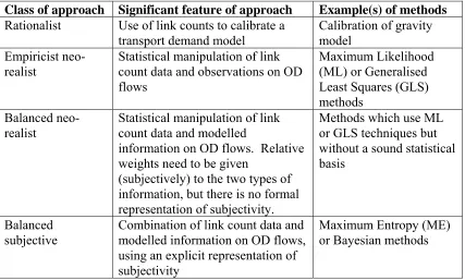
By combining the two different types of classification, and discarding combinations that are not useful (such as empiricist subjectivity), we can list the following approaches to be used for the review in Section 5:
• Rationalist
• Empiricist neo-realist
• Balanced neo-realist
6.4.1 Rationalist
The rationalist approach concerns using link counts to calibrate a model, which keeps its structure after the calibration process. The approach could involve the transport planner using either a neo-realist or subjective attitude towards the model concerned. In the neo-realist case, s/he would be 'pretending' that it was true (in a realist sense), whilst in the subjective case s/he would use it because that is what society (or the relevant social group) would expect her/him to do. Whilst the latter position appears more sound, the actual numerical results produced would be the same in both cases. However, the actual interpretation of the results would be different.
6.4.2 Empiricist neo-realist
Empiricist neo-realist methods essentially involve statistical manipulation of link count observations and trip matrix observations, using standard statistical sampling methods. As pointed out above (in (4.3.2)), such methods are 'nearer to realism' than balanced or rationalist neo-realist approaches. Whilst they are in a sense more scientifically justifiable, they rely heavily upon the availability of large amounts of observed data.
6.4.3 Balanced neo-realist
Balanced neo-realist approaches make a matrix estimation by combining a matrix estimation model with link count observations. Unlike rationalist methods, the prior model structure is liable to disappear from the final estimated matrix, due to the influence of the link count data. Two cases can be identified. If the link count observations are assumed to be completely accurate, the problem is constrained in the sense that the solution must satisfy the constraints imposed by the link counts. Practically, this assumption of complete accuracy only needs to be made relative to the quality of information from the model. However, this type of relativist
assumption might be awkward for some method-users (especially if they know for certain that the link counts are inaccurate), since it contains an element of subjectivity which does not fit comfortably within the philosophy behind neo-realist models.
given in Section 5) is that there is a confusion as to whether the prior matrix distribution refers to the variation in the trip matrix cells or to uncertainty about the mean trip rate.
6.4.4 Balanced subjective
As with the balanced neo-realist methods, we can identify two different types of balanced subjective method, depending upon whether we assume the link counts are completely accurate or not. An important difference between the two approaches (neo-realist and subjective) is that, in the subjective case, it is completely within the philosophy of the method to make a relativist assumption that the link counts are only accurate in comparison with the prior (model) information.
In the constrained case, the subjective methods considered in this paper are Maximum Entropy (ME) methods. In such methods, a matrix is estimated which is as near as possible to a prior matrix (which is created from the professional judgement of the transport planner) and which conforms precisely to the link count observations. Methods have also been developed which extend the basic ME methods to unconstrained problems. In such extensions, the user must attach weights to the model information and to the observed information. However, such a process undermines the conceptual simplicity and coherence of ME which relies upon absolute precedence of observed information over subjective information. This basic philosophical problem translates into a practical problem in that the process is not obvious by which the user decides upon the relative weights to attach to modelled and observed information. Arguably, the extended ME approach is an ad-hoc approach which does not fit into any formally subjective method, and has more in common with the balanced neo-realist approaches described above. However, since this might be disputed and since it is logically sensible to describe such methods after describing the basic ME method, they are included (in Section 5) pragmatically in the sub-section on subjective methods.
On the other hand, the Bayesian approach is an internally coherent method for representing the trade-off between personal belief (as expressed by the prior distribution) and observations, in the knowledge that the observations have various uncertainties attached to them. Whilst the decision about the values of the weights to put on modelled information is inevitably still problematic, the process by which this is done is extremely transparent for the method-user. In simple terms, it represents the process experienced in our everyday lives of updating our views on the world in response to new information.
7. REVIEW OF METHODS
7.1 Introduction
Section 5 is concerned with how the philosophical approaches, described in Section 4, have been applied in various methods for matrix estimation using link counts. A review of published material on the subject is presented, covering the last 30 years. A number of points can be raised at the outset:
• The practical orientation of this paper leads it to consider mainly those methods where there is an important need for philosophical understanding. These are the methods that are required for dealing with 'more complex applications' in the terms described in Section 3. It follows then that there will be little reference below to methods that deal principally with small network applications (where assignment characteristics are dictated by the nature of the network, and where there is often no need for a prior matrix). As stated in (3.2), two prime examples of this type of application are: the estimation of turning movements at junctions; and the estimation of an entry-exit matrix for a motorway. An important set of methods for dealing with such problems has been labelled by Zhang and Maher (1998a) as
semi-disaggregate, and includes methods by Cremer and Keller (1987), Nihan and Davis (1987 and 1989), and Bell (1991a).
• As we move from the high philosophical perspective of Section 4 to a more practical methodological perspective in Section 5, more importance gets attached to whether or not we are dealing with constrained methods. The choice between constrained and unconstrained methods will typically depend upon the application for using the method. Thus, if we have (accurate) link flow counts of road vehicles and we are wishing to estimate a road vehicle trip matrix, there is greater impetus for using a constrained method than in many other applications (where the 'link counts' are likely to be less reliable). With the greater emphasis on this issue, the four essential approaches given in (4.4) are extended to six method-types, with the balanced approaches being distinguished as to whether they are constrained or unconstrained:
• Rationalist
• Empiricist neo-realist
• Balanced neo-realist (constrained)
• Balanced neo-realist (unconstrained)
• Balanced subjective (constrained)
• Balanced subjective (unconstrained).
• Reference is given in a number of places to where differing (philosophical) approaches lead to mathematically coincidental objective functions, or at least first-order approximations of each other. The potential confusion arising from this issue has already been discussed above in (4.1).
• In line with the remainder of this paper, 'link counts' are often referred to as if they were the only source of observational data. However, following the 'unified framework' approach discussed in (3.5) above, most of the methods described below are easily extended to take into account other forms of observational data.
7.2 Rationalist
A summary of attempts, arising in the 1970’s, to use link count data to calibrate gravity models is given by Willumsen (1981). He writes that the simplest form of gravity model can be written as:
(5.1) Tij = b O D c1 i j ij−d
where:
Oi represents origin information
Dj represents destination information
cij is the cost of travel between i and j
b1 and d are parameters to be calibrated
Willumsen then shows that link count information can be used through the following equation to calibrate (5.1):
(5.2)
Fa b T pij ija
ij
= 0 + ∑
where:
b0 represents local (intrazonal) traffic
Fa and pija are as defined in eqn (2.1)
If a set of link count observations {F$a} are made, optimal values of b0, b1 and d can
be found by minimising the sum of squared differences between { } and the corresponding modelled values {F
$ Fa
a}. Variations of this method are reported in Low
(1972), Hogberg (1976) and Holm et al (1976).
7.3 Empiricist neo-realist
In their highly informative 'Unified framework for estimating or updating origin/destination matrices from traffic counts', Cascetta and Nguyen (1988) consider two main types of classical statistical technique for the static estimation problem:
• The maximum likelihood (ML) method
• The generalised least squares (GLS) method
In a follow-up paper (Cascetta et al, 1993), the framework is extended to include within-day dynamics.
7.3.1 Maximum likelihood method
By making assumptions about (probability) distributions of link flows and O-D flows, we can construct, for any set of observations we have, a likelihood function L of making those observations. In particular, if we have observed link counts { } and
O-D counts { } and we assume that these counts are statistically independent, then
we have:
$ Fa
$ Nij
(5.3) L F({$a},{N$ij} / { })Tij = L F({$a} / { }) *Tij L N({$ ij} / { })Tij
By maximising (5.3) with respect to {Tij}, we can compute the most likely values of
{Tij}. Alternatively, the ML estimator can often be found more conveniently by
maximising the natural logarithm of (5.3), giving us the optimisation problem:
(5.4)
wrt Tij a ij ij ij
Maximise LogL F T LogL N T
{ }
({$ } / { }) + ({$ } / { })
Spiess (1987) uses such a technique, taking explicit account of the sampling factors used when the OD counts are made. He assumes that the observations { } have
been made upon mutually independent Poisson distributed random variables with means {ρ
$ Nij
ijTij}, where {ρij} are the sample factors for the counts. Initially he assumes
that the link flows have been sampled to such an extent that their means {Fa} are
known with certainty. The likelihood of observing {N$ij} is thus given by:
( )
$ !
$
ρij ij N ρT
ij ij
T e
N
ij − ij ij
∏
(5.5)and he obtains the problem:
(5.6)
wrt Tij ij ij ij ij ij
Min T N LogT
{ } (
$ )
ρ −
subject to eqn (2.1), and
Tij≥0 (5.7)
The solution to this problem is:
T N
p
ij
ij
ij ija a
a
* = $
+ ∑
ρ λ (5.8)
where {λa} are 'balancing factors' created by the 'conflict' of {N$ij} and {Fa}. Hence,
if the information from { } is entirely compatible with the link count observations,
each λ
$ Nij
a = 0. It can be seen from eqn (5.8) that this would give us, as we would
expect, the solution:
(5.9) Tij* = N$ij /ρij
If {Fa} are not known with certainty, Spiess derives the more generalised problem:
(5.10)
wrt Tij ij ij ij ij ij a a a a a
Min T N LogT F M LogF
{ }
(ρ − $ ) (ρ $ )
∑ + ∑ −
⎛ ⎝
⎜ ⎞⎠⎟
subject to eqn (2.1)
where:
ρa is the sampling factor of the flow along link a;
{ } are observations on mutually independent Poisson distributed random
variables with means {ρ $
Ma
aFa}.
Other writers using an ML approach include:
• Landau et al (1982) who assume that O-D flows have a Multinomial distribution;
• Nguyen et al (1988) who make similar distributional assumptions to Spiess for a problem that is specifically concerned with public transport bus passengers, both in terms of the network representation and the assignment model used;
• Lo et al (1996 and 1999) who develop an ML approach which considers the link choice proportions {pija} as random variables;
• Hazleton (2000) who describes an ML method which relies solely on link counts, thus not requiring observations on {Tij} (although it can be extended to use such
7.3.2 Generalised Least Squares
Cascetta (1984) gives an example of a GLS estimator as follows. Using vector/matrix notation (so that {Tij} becomes T, and {Fa} becomes F etc), we can specify:
(5.11)
$
T = T+ η
(5.12)
$
F = F+ ε
where η and ε are disturbance vectors of dimensions n2 and m respectively.
Suppose that we ignore measurement error. Since we have defined T and F as means, it follows that:
E( )η = E( )ε = 0 (5.13)
It is an advantage of the GLS technique that no (probability) distributional assumptions need to made about link flows and O-D flows. However, this advantage is qualified in that it is necessary to make assumptions as to the variance-covariance matrices of η and ε.
Assume then that the variance co-variance matrices of η and ε are Z and W respectively. Then the GLS estimator of T is found by solving the following minimisation problem:
(5.14)
(
)
wrt
Min
T
1
(T$ −T)Z (T− $ −T)+(F$ −F)W−1(F$ −F)
c
Cascetta and Nguyen (1988) point out that the estimator in eqn (5.14) coincides mathematically with the Maximum Likelihood Estimator when Multivariate Normal distributional assumptions are made for and . A problem with this estimator is that it can produce negative estimates for some trip matrix cells. To overcome this problem, formal non-negativity constraints need to be imposed upon eqn (5.14), hence leading to a potentially more complicated solution procedure. Bell (1991b) describes a procedure for solving (5.14) subject to
$
T F$
T ≥ (5.15)
where c represents a generalised set of lower bounds on T.
derived from any source, and not just from direct observations). Discussion of such methods will be deferred to (5.4) and (5.5).
7.4 Balanced neo-realist (constrained)
Carey and Revelli (1986) consider the following linear direct demand distribution model:
T = Xβ + ε (5.16)
where:
X is an (n2 x s) matrix consisting of n2 observations on each of s socioeconomic variables;
β is a vector of parameters (of dimension s);
ε is a vector of random disturbances (with assumed zero mean) (of dimension n2).
Eqn (5.16) is constrained by observations:
c = AT (5.17)
where:
c is a vector of observations (of dimension m); A is an (m x n2) matrix of known constants.
Clearly, the constraint set is defined in a generalised way and concerns observations on any linear combination of elements of T: observations on link flows are simply a special case.
It is useful to point out here that if there were no ε in eqn (5.16), the method would be classed as rationalist (as defined in Section 4).
The following estimation problem arises:
wrt ,
Minimise
Tβ
(T−X )V (−1 T−X ) (5.18)
subject to eqn (5.16) and:
7.5 Balanced neo-realist (unconstrained)
7.5.1 Least squares methods
Further to their consideration of the constrained case, Carey and Revelli (1986) also consider an unconstrained case, extending eqn (5.17) to:
c = AT + u (5.20)
where u is a random disturbance factor.
A similar method is described by Hendrickson and McNeil (1984). In particular they consider the case where the parameters β (in eqn (5.16)) are 'known', so that the minimisation problem in eqn (5.18) simplifies to:
(5.21)
wrt
Min
T
(T−y)V (−1 T−y)
)
= subject to eqns (5.15) and (5.19)
where y are the model hypothesised values of O-D flows.
Suppose that the matrix V is written as {vkl}. Then Hendrickson and McNeil show
that if:
vkl = 0 ∀k≠l
vkk = yk ∀k
where yk is the kth element of y,
then we obtain the problem:
(
wrt k k k k
Minimise T y y s t
T
c AT
− ∑ ⎡ ⎣⎢
⎤ ⎦⎥
) /2 . . (5.22)
where Tk is the kth element of T.
They point out that the objective function in eqn (5.22) is a first-order approximation to the negative of the entropy function (to be discussed below in Section 5.6):
T Log T y
k
k
k k
⎛ ⎝
⎜ ⎞
⎠ ⎟
∑ (5.23)
7.5.2 Maximum likelihood methods
The MVESTM method (which is part of the TRIPS suite of programmes), has been described by Logie and Hynd (1990), Logie (1993), and Smith and Logie (1993). This method is based upon the mathematical formulation given by Spiess (1987), described in (5.3.1) above. However, the MVESTM method is not restricted to problems which only use directly observed data (as considered by Spiess). The MVESTM method embodies the 'unified framework' spirit described in (3.4) and can update a prior matrix by using: link flow counts; public transport passenger counts; a trip cost matrix (if surveyed journey time data is available); directly observed trip matrix cells; trip end counts; and part-trip data.
7.6 Balanced subjective (constrained)
7.6.1 Basic method
The only constrained balanced subjective method considered here is the maximum entropy method. Cascetta and Nguyen (1988) define the 'generic maximum entropy trip matrix estimation problem' to be:
wrt T ij
ij
ij ij
ij
Maximise T Log T q
{ }
− ⎛
⎝ ⎜⎜ ⎞⎠⎟⎟
∑ (5.24)
subject to:
∀a∈A (2.1)
a ij
ij ija
F = ∑T p
∀ij (5.25)
Tij ≥ 0
(5.26) Tij
ij
∑ = constant
where {qij} are prior estimates of {Tij}.
Much of the groundwork for using an entropy approach to estimate OD matrices was laid by Wilson (1970) who considered the special case in which {qij} are all (by
definition) equal to one another, so that there is effectively no prior information on {Tij}. Thus eqn (5.24) becomes:
(5.27)
wrt Tij ij ij ij
Maximise T LogT
{ }
− ∑
subject to eqns (5.25) and (5.26) and appropriate constraints.
Wilson did not in fact use link count constraints (of the type given in eqn (2.1)), but used constraints resulting from counts on origin and destination totals..
leaving it with many of its physical science restrictions. The full adaptation of the method to social science was made by Willumsen, who used the maximum entropy technique with prior information (in the form of differing {qij}) and link count
constraints. At the same time, similar work was being carried out by Van Zuylen using Information Theory. The collaboration of the two lines of research resulted in a joint paper (Van Zuylen and Willumsen, 1981). The solution to 'Willumsen’s problem' is:
Tij qij Xap (5.28)
a
ija
= ∏
where {Xa} are 'balancing factors' which are calculated within the solution method.
The values of {Xa} depend upon how well the prior matrix {qij} is consistent with the
link counts {Fa}. If the {qij} are entirely consistent with {Fa}, {Xa} all have value 1.
Essentially, this is the method used by the ME2 programme within the SATURN suite (Van Vliet and Hall, 1998). Following the 'unified framework' approach, the ME2 method can also make use of origin count constraints, destination count constraints, turning movement constraints (at junctions) and constraints on individual cells of {Tij}. However, in real life applications, it is unlikely that the set of eqns (2.1) and
other constraint equations will be internally consistent. Thus, the idealised formulation of a 'precisely constrained' problem needs to be somewhat relaxed. ME2 (as applied in SATURN) takes an expedient approach towards this problem by setting (user-defined) minimum and maximum values on {Xa}. Implicitly, the method thus
becomes unconstrained. However the underlying message to the method-user is that observed link count information is more reliable than prior information (in accordance with the basic ME method). For urban road traffic applications (the main focus of SATURN’s use), this approach can arguably be considered as reasonably pragmatic. Furthermore, it can be argued that it is only when different applications need to be considered (such as public transport passenger matrix estimation) that there is a requirement to make explicit recognition of uncertainty in counts.
7.6.2 Methods that recognise growth
Many methods have been consciously concerned with updating an old matrix {tij}
using link count data. An important defect of many of the original methods for doing so was that there was no explicit representation of growth between the time that the old matrix was estimated and the 'present'. Thus, in practice, the 'old' matrix {tij} was
confused with the 'prior' matrix {qij}, so that {tij} was used instead of {qij} in eqn
(5.28). If the flow between a particular ij pair does not pass through any count point it can be seen immediately from eqn (5.28) that Tij is fixed at tij. If tij is 'known' by the
method-user to be too small (or too large) an estimate of Tij (since s/he knows that
Two general approaches to solving this problem have been used. Firstly, the old matrix can be updated exogenously. This is the approach taken by ME2 in SATURN. Secondly, the link counts can be used to provide information about growth as part of the estimation process. Early examples of such an approach are given by Van Zuylen (1981) and Bell (1983) who consider a problem:
Tij tij Xap
a
ija
= τ ∏ (5.29)
where τ =
∑
∑
T
t
ij ij
ij ij
(5.30)
Thus, no prior information on τ is required by the estimation process. A more complex procedure (though still not requiring prior information on growth) was devised by Maher (1987) who considered the problem:
Tij A B ti j ij Xap
a
ija
= ∏ (5.31)
where A
T
t and B
T
t
i
ij j
ij j
j
ij i
ij i =
∑
∑ =
∑
∑ (5.32)
7.6.3 Other (constrained) extensions
It is generally recognised that assignment proportions {pija} are likely to vary between
7.7 Balanced subjective methods (unconstrained).
Two types of method are considered in this section. Firstly, there are methods based upon extending maximum entropy techniques to the case where link count observations cannot be considered to yield fixed constraints. Secondly, there are Bayesian methods.
7.7.1 'Unconstrained' maximum entropy
Willumsen (1984), Hamerslag and Immers (1988) and Brenninger-Göthe et al (1989), all consider extensions of the ME problem of the type:
wrt T ij
ij ij ij a a a a ij
Minimise T Log T
q F Log
F
F
{ } $
γ1 ⎛ γ2
⎝ ⎜⎜ ⎞⎠⎟⎟ ∑ + ⎛ ⎝ ⎜ ⎞ ⎠ ⎟ ∑ ⎡ ⎣ ⎢ ⎢ ⎤ ⎦ ⎥
⎥ (5.33)
s.t. eqns (2.1) and (5.25), where γ1 and γ2 are weighting factors.
Jörnsten and Wallace (1993) describe a further development of the type of approach given in eqn (5.33), taking explicit account of the fact that individual counts have differing degrees of quality (typically as a result of the sampling factors used when making the counts). Heydecker et al (1994) extend this approach by also taking into account differences in quality between individual {qij}, thus yielding a problem of the
type: ⎥ ⎥ ⎦ ⎤ ⎢ ⎢ ⎣ ⎡ ∑ ⎟⎟ ⎠ ⎞ ⎜ ⎜ ⎝ ⎛ + ∑ ⎟⎟ ⎠ ⎞ ⎜ ⎜ ⎝ ⎛ a a a a a ij ij ij ij ij } {T
wrt Fˆ
F Log F q T Log T Minimise ij (5.34)
Whilst such methods might be intuitively attractive extensions of the basic ME method, they do not appear to have a strong theoretical basis, lying somewhere in between standard statistical approaches (of the type described in (5.3)) and a standard ME approach. In (4.4.4) it was questioned whether such methods were formally subjective. The practical consequence of this uncertainty is that the method-user has no clear process for allocating numerical estimates to γ1 in eqn (5.33) or {γij} in eqn
(5.34).
7.7.2 Bayesian methods
Probably the first example of a Bayesian approach towards trip matrix estimation using link count data was developed by Maher (1983), who made Multivariate Normal assumptions for both the prior distribution of T and the conditional distribution of link flows (with mean F). Thus if:
T ~ MVN(µ0,V0)
(5.35)