Chapter 9
Na¨ıve Bayes
David J. Hand
Contents
9.1 Introduction . . . .163
9.2 Algorithm Description . . . .164
9.3 Power Despite Independence . . . .167
9.4 Extensions of the Model . . . .169
9.5 Software Implementations. . . .171
9.6 Examples . . . .171
9.6.1 Example 1 . . . .171
9.6.2 Example 2 . . . .173
9.7 Advanced Topics. . . .174
9.8 Exercises . . . .175
References . . . .176
9.1
Introduction
Given a set of objects, each of which belongs to a known class, and each of which has a known vector of variables, our aim is to construct a rule which will allow us to assign future objects to a class, given only the vectors of variables describing the future objects. Problems of this kind, called problems of supervised classification, are ubiquitous, and many methods for constructing such rules have been developed. One very important method is the na¨ıve Bayes method—also called idiot’s Bayes,
simple Bayes, and independence Bayes. This method is important for several reasons,
breast cancer recurrence. Many further examples showing the surprising effectiveness of the na¨ıve Bayes method are listed in Hand and Yu (2001) and further empirical comparisons, with the same result, are given in Domingos and Pazzani (1997). Of course, there are also some other studies which show poorer relative performance from this method: For a comparative assessment of such studies, see Jamain and Hand (2008).
For convenience, most of this chapter will describe the case in which there are just two classes. This is, in fact, the most important special case as many situations naturally form two classes (right/wrong, yes/no, good/bad, present/absent, and so on). However, the simplicity of the na¨ıve Bayes method is such that it permits ready generalization to more than two classes.
Labeling the classes by i =0,1, our aim is to use the initial set of objects which
have known class memberships (known as the training set) to construct a score such that larger scores are associated with class 1 objects (say) and smaller scores with class 0 objects. New objects are then classified by comparing their score with a “classification threshold.” New objects with a score larger than the threshold will be classified into class 1, and new objects with a score less than the threshold will be classified into class 0.
There are two broad perspectives on supervised classification, termed the diagnostic
paradigm and the sampling paradigm. The diagnostic paradigm focuses attention on
the differences between the classes—on discriminating between the classes—while the sampling paradigm focuses attention on the individual distributions of the classes, comparing these to indirectly produce a comparison between the classes. As we show below, the na¨ıve Bayes method can be viewed from either perspective.
9.2
Algorithm Description
Beginning with the sampling paradigm, define P(i|x) to be the probability that an
object with measurement vector x=(x1, . . . ,xp) belongs to class i , f (x|i ) to be the
conditional distribution of x for class i objects, P(i ) to be the probability that an object will belong to class i if we know nothing further about it (the “prior” probability of class i ), and f (x) to be the overall mixture distribution of the two classes:
f (x)= f (x|0)P(0)+ f (x|1)P(1)
Clearly, an estimate of P(i|x) itself would form a suitable score for use in a
9.2 Algorithm Description 165
A simple application of Bayes theorem yields P(i|x)= f (x|i )P(i )/f (x), and to
obtain an estimate of P(i|x) from this, we need to estimate each of the P(i ) and each
of the f (x|i ).
If the training set is a simple random sample drawn from the overall population distribution f (x), the P(i ) can be estimated directly from the proportion of class i objects in the training set. Sometimes, however, the training set is obtained by more complicated means. For example, in many problems the classes are unbalanced, with one being much larger than the other (e.g., in credit card fraud detection, where only 1 in 1,000 transactions may be fraudulent; in rare disease detection, where the ratio may be even more extreme; and so on). In such cases, the larger of the two classes is often subsampled. For example, perhaps only 1 in 10 or 1 in 100 of the larger class will be used in the training set. If this is the case, then it is necessary to reweight the simple observed proportion in the training set to yield an estimate of P(i ). In general, if the observations are not drawn as a simple random sample from the training set, some thought will need to go into how best to estimate the P(i ).
The core of the na¨ıve Bayes method lies in the method for estimating the
f (x|i ). The na¨ıve Bayes method assumes that the components of x are
indepen-dent within each class, so that f (x|i )=pj=1 f (xj|i )—hence the alternative name
of “independence Bayes.” Each of the univariate marginal distributions, f (xj|i ),
j =1, . . . ,p; i =0,1, is then estimated separately. By this means, the p
dimen-sional multivariate problem is reduced to p univariate estimation problem. Univariate estimation is familiar and simple, and requires smaller training set sizes to obtain accurate estimates than does the estimation of multivariate distributions.
If the marginal distributions f (xj|i ) are discrete, with xjtaking only a few values,
one can estimate each of the f (xj|i ) by simple multinomial histogram-type estimators.
Because this is so straightforward, this is a very common approach to the na¨ıve Bayes estimator, and many implementations adopt this approach. Indeed, it is so straightforward that many implementations partition any continuous variables (age, weight, income, and so on) into cells so that a multinomial histogram-type estimator can be constructed for all of the variables. At first glance, this strategy might seem to be a weak one. After all, it means that any notion of continuity between neighboring cells of the histogram has been sacrificed. It also requires the cells to be wide enough to contain sufficient data points that accurate probability estimates can be obtained. On the other hand, it can be regarded as providing a very general nonparametric estimate of the univariate distribution, so avoiding any distributional assumptions. In particular, it is a nonlinear transformation, so that, for example, the relationship
between estimates of f (xj|i ) does not need to be monotonic in xj.
said that, there is another reason why one might prefer to use the histogram approach based on forcing all the variables to be discrete—that of interpreting the results. We discuss this below.
The assumption of independence at the core of the na¨ıve Bayes method is clearly a strong one. It is unlikely to be true for most real problems. (How often does a diagonal covariance matrix arise from real data in practice?) A priori, then, one might expect the method to perform poorly precisely because of this improbable assumption lying at its core. However, the fact is that it often does surprisingly well in real practical applications. Reasons for this counterintuitive result are discussed below.
So far we have approached the na¨ıve Bayes method from the sampling paradigm, describing it as being based on estimating the separate class conditional distributions using the simplifying assumption that the variables in each of these distributions were independent. However, the elegance of the na¨ıve Bayes method only really becomes apparent when we note that we can obtain classifications equivalent to the above if we
use any strictly monotonic transformation of P(i|x), transforming the classification
threshold in a similar way. To see this, note that if T is a strictly monotonic increasing transformation then
P(i|x)>P(i|y) ⇔ T (P(i|x))>T (P(i|y))
and, in particular, P(i|x)>t ⇔ T (P(i|x))>T (t). This means that if tis the
classifi-cation threshold with which P(i|x) is compared, then comparing T (P(i|x)) with T (t)
will yield the same classification results. (We will assume only monotonic increasing transformations, though the extension to monotonic decreasing transformations is trivial.)
One such monotonic transformation is the ratio
P(1|x)/(1−P(1|x))=P(1|x)/P(0|x) (9.1)
Using the na¨ıve Bayes assumption that the variables within each class are indepen-dent, so that the distribution for class i has the form f (x|i )=pj=1 f (xj|i ), the ratio P(1|x)/(1−P(1|x)) can be rewritten:
P(1|x)
1−P(1|x) =
P(1)pj=1 f (xj|1) P(0)pj=1 f (xj|0)
= P(1)
P(0) p
j=1
f (xj|1) f (xj|0)
(9.2)
The log transformation is also monotonic (and combination of monotonic functions yields monotonic functions) so that another alternative score is given by
ln P(1|x)
1−P(1|x) =ln
P(1)
P(0)+
p
j=1
lnf (xj|1)
f (xj|0)
(9.3)
If we definewj(xj)=ln( f (xj|1)/f (xj|0)) and k =ln{P(1)/(P(0))}we see that
Equation (9.3) takes the form of a simple sum
ln P(1|x)
1−P(1|x)=k+
p
j=1
9.3 Power Despite Independence 167
of contributions from the separate variables. Since the score S =k+pj=1wj(xj)
is a direct estimate of (a monotonic transformation of) P(1|x), it is based on the
diagnostic paradigm. The ease of interpretation now becomes apparent: The na¨ıve
Bayes model is simply a sum of transformed values of the raw xjvalues.
In cases when each variable is discrete, or is made to be discrete by partitioning it
into cells, Equation (9.4) takes a particularly simple form. Suppose that variable xj
takes a value in the kjth cell of the variable, denoted x
(kj)
j . Thenwj(x
(kj)
j ) is simply
a logarithm of a ratio of proportions: the proportion of class 1 points which fall into
the kjth cell of variable xj divided by the proportion of class 0 points which fall into
the kjth cell of variable xj. Thesewj(x
(kj)
j ) are called weights of evidence in some
applications:wj(x
(kj)
j ) shows the contribution the j th variable makes toward the total
score, or the evidence in favor of the object belonging to class 1 that is provided by the j th variable. Such weights of evidence are useful in identifying which variables are important in assigning any particular object to a class. (This is vital in some applications, such as credit scoring in personal banking, where the law requires that reasons must be given if an application for a loan is declined.)
9.3
Power Despite Independence
The assumption of independence of the xj within each class implicit in the na¨ıve
Bayes model might seem unduly restrictive. After all, as noted above, variables are rarely independent in real problems. In fact, however, various factors may come into play which means that the assumption is not as detrimental as it might seem (Hand and Yu, 2001).
Firstly, the complexity of p-univariate marginal distributions is far lower than that of a single p-variate multivariate distribution. This means that far fewer data points are needed to obtain a given accuracy under the independence model than are needed without this assumption. Put another way, the available sample will lead to an esti-mator with smaller variance if one is prepared to restrict the model form by assuming independence of the variables within classes. Of course, if the assumption is not true, then there is a risk of bias. This is a manifestation of the classic bias/variance trade-off, which applies to all data analysis modeling, and is not specific to the na¨ıve Bayes model.
To decrease the risk of bias arising from the assumption of independence, a simple modification of the basic na¨ıve Bayes model has been proposed. To understand the reasoning behind this modification, consider the special case in which the marginal distributions of all the variables are the same, and the extreme in which the variables are perfectly correlated. This means that, for any given class, the probability that the
case, the na¨ıve Bayes estimator is
P(1|x)
P(0|x) =
P(1) P(0)
f (xk|1)
f (xk|0)
p
while the true odds ratio is
P(1|x)
P(0|x) =
P(1) P(0)
f (xk|1)
f (xk|0)
for any k∈ {1, . . . ,p}. We can see from this that if f (xk|1)/f (xk|0) is larger than 1, the
presence of correlation will mean that the na¨ıve Bayes estimator tends to overestimate
P(1|x)/P(0|x), and if f (xk|1)/f (xk|0) is less than 1, the presence of correlation will
mean that the na¨ıve Bayes estimator tends to underestimate P(1|x)/P(0|x). This
phenomenon immediately suggests modifying the na¨ıve Bayes estimator by raising
the f (xk|1)/f (xk|0) ratios by some power less than 1, to shrink the overall estimator
toward the true odds. In general, this yields the improved na¨ıve Bayes estimator
P(1|x)
P(0|x) =
f (x|1)P(1)
f (x|0)P(0) =
P(1) P(0)
p
j=1
f (xj|1) f (xj|0)
β
withβ <1.βis typically chosen by searching over possible values and choosing that which gives best predictive results by means of a method such as cross-validation. We can also see that this leads to a shrinkage factor appearing as a coefficient of the
wj(xj) terms in Equation (9.4).
A second reason why the assumption of independence is not as unreasonable as might at first seem is that often data might have undergone an initial variable selection procedure in which highly correlated variables have been eliminated on the grounds that they are likely to contribute in a similar way to the separation between classes. Think of variable selection methods in linear regression, for example. This means that the relationships between the remaining variables might well be approximated by independence.
A third reason why the independence assumption may not be too detrimental is that only the decision surface matters. While the assumption might lead to poor estimates
of probability or of the ratio P(1|x)/P(0|x), this does not necessarily imply that
the decision surface is far from (or even different from) the true decision surface. Consider, for example, a situation in which the two classes have multivariate normal distributions with the same (nondiagonal) covariance matrix, and with the vector of differences between the means lying parallel to the first principal axis of the covariance matrix. The optimal decision surface is linear and is the same with the true covariance matrices and under the independence assumption.
Finally, of course, the decision surface produced by the na¨ıve Bayes model can in
fact have a complicated nonlinear shape: The surface is linear in thewj(xj) but highly
9.4 Extensions of the Model 169
9.4
Extensions of the Model
We have seen that the na¨ıve Bayes model is often surprisingly effective. It also has the singular merit of being very easy to compute, especially if the discrete variable version is used. Coupled with the ease of understanding and interpretation of the model, perhaps especially in terms of the simple points-scoring perspective in Equation (9.4), these factors explain why it is so widely used. However, its very simplicity, along with the fact that its core assumption often appears unrealistic, has led many researchers to propose extensions of it in an attempt to improve its predictive accuracy.
We have already seen one of these above, to ease the independence assumption by shrinking the probability estimates. Shrinking has also been proposed to improve the simplistic multinomial estimate of the proportions of objects falling into each category in the case of discrete predictor variables. So, if the j th discrete predictor
variable, xj, has cr categories, and if njr of the total of n objects fall into the r th
category of this variable, the usual multinomial estimator of the probability that a
future object will fall into this category, njr/n, is replaced by (njr+cr−1)/(n+1).
This shrinkage, which is also sometimes called the Laplacian correction, also has a direct Bayesian interpretation. It can be useful if the sample size and cell widths are such that there may not be very many objects in a cell.
Perhaps the most obvious way of easing the independence assumption is by intro-ducing extra terms in the models of the distributions of x in each class, to allow for interactions. This has been attempted in a large number of ways, but all of them nec-essarily introduce complications, and so sacrifice the basic simplicity and elegance of the na¨ıve Bayes model. In particular, if an interaction between two of the variables in x is to be included in the model, then the estimate cannot be based merely on the univariate marginals.
Within the i th class, the joint distribution of x is
f (x|i )= f (x1|i ) f (x2|x1,i ) f (x3|x1,x2,i ). . . f (xp|x1,x2, . . . ,xp−1,i ) (9.5) and this can be approximated by simplifying the conditional probabilities. The extreme arises with f (xj|x1, . . . ,xj−1,i ) = f (xj|i ) for all j , and this is the na¨ıve Bayes
method. Obviously, however, models between these two extremes can be used. If the variables are discrete, one can estimate appropriate models, with arbitrary degrees of interaction included, by using log-linear models. For continuous variables, graphical models and the literature on conditional independence graphs are appropriate. An example which is appropriate in some circumstances is the Markov model
f (x|i )= f (x1|i ) f (x2|x1,i ) f (x3|x2,i ), . . . , f (xp|xp−1,i ) (9.6) This is equivalent to using a subset of two-way marginal distributions instead of merely the univariate marginal distributions in the na¨ıve Bayes model.
to each subset. Such models are popular in some applications, where they are known as segmented scorecards. The segmentation is a way to allow for interactions which would cause difficulties if a single overall independence model was fitted.
Another way of embedding na¨ıve Bayes models in higher-level approaches is by means of multiple classifier systems, for example, in a random forest or via boosting. There is a very close relationship between the na¨ıve Bayes model and another very important model for supervised classification: the logistic regression model. This was originally developed within the statistical community, and is very widely used in medicine, banking, marketing, and other areas. It is more powerful than the na¨ıve Bayes model, but this extra power comes at the cost of necessarily requiring a more complicated estimation scheme. In particular, as we will see, although it has the same attractively simply basic form as the na¨ıve Bayes model, the parameters (e.g., thewj(x
(kj)
j )) cannot be estimated simply by determining proportions, but require an
iterative algorithm.
In examining the na¨ıve Bayes model above, we obtained the decomposition Equation (9.2) by adopting the independence assumption. However, exactly the same
structure for the ratio results if we model f (x|1) by g(x)pj=1h1(xj) and f (x|0) by
g(x)pj=1h0(xj), where the function g(x) is the same in each model. If g(x) does
not factorize into a product of components, one for each of the raw xj, we are not
assuming independence of the xj. The dependence structure implicit in g(x) can be
as complicated as we like—the only restriction being that it is the same in the two
classes; that is, that g(x) is common in the factorizations of f (x|1) and f (x|0). With
these factorizations of the f (x|i ), we obtain
P(1|x)
1−P(1|x) =
P(1)g(x)pj=1h1(xj) P(0)g(x)pj=1h0(xj)
= P(1)
P(0).
p
j=1h1(xj)
p
j=1h0(xj)
(9.7)
Since the g(x) terms cancel, we are left with a structure identical to Equation (9.2),
although the hi(xj) are not the same as the f (xj|i ) (unless g(x)≡1). Note that in this
factorization it is not even necessary that the hi(xj) be probability density functions.
All that is needed is that the overall products g(x)pj=1hi(xj) are densities.
The model in Equation (9.7) is just as simple as the na¨ıve Bayes model, and takes exactly the same form. In particular, by taking logs we end up with a points-scoring model as in Equation (9.4). But the model in Equation (9.7) is more flexible than
the na¨ıve Bayes model because it does not assume independence of the xj in each
class. Of course, this considerable extra flexibility of the logistic regression model is not obtained without cost. Although the resulting model form is identical to the na¨ıve Bayes model form (with different parameter values, of course), it cannot be estimated by looking at the univariate marginals separately: An iterative procedure must be used. Standard statistical texts (e.g., Collett, 1991) give algorithms for esti-mating the parameters of logistic regression models. Often an iterative proportional weighted least squares method is used to find the parameters which maximize the likelihood.
The version of the na¨ıve Bayes model based on the discretization transformation of
9.5 Software Implementations 171
class of generalized additive models (Hastie and Tibshirani, 1990) take exactly the
form of additive combinations of transformations of the xj.
The na¨ıve Bayes model is tremendously appealing because of its simplicity, ele-gance, robustness, as well as the speed with which such a model can be constructed, and the speed with which it can be applied to produce a classification. It is one of the oldest formal classification algorithms, and yet even in its simplest form it is often surprisingly effective. A large number of modifications have been introduced, by the statistical, data mining, machine learning, and pattern recognition communities, in an attempt to make it more flexible, but one has to recognize that such modifications are necessarily complications, which detract from its basic simplicity.
9.5
Software Implementations
The simplicity of the na¨ıve Bayes algorithm means that, in its basic form, it has been very widely implemented, and many free versions are available on the Web. The open-source Weka implementation (http://www.cs.waikato.ac.nz/ml/weka/) allows the individual variables to be modeled by normal distributions, by kernel estimates, or by splitting them into discrete categories.
Perhaps it is worthwhile making a cautionary comment. The term Bayesian has sev-eral different interpretations, and its now common use in the phrase “na¨ıve Bayes clas-sifier” can mislead the unwary. In particular, “Bayesian networks” are more general classes of models, which include the na¨ıve Bayes model as a special case, but which generally also allow various interactions to be included in the model. An example of the sorts of confusion this can lead to is described in Jamain and Hand (2005).
9.6
Examples
9.6.1
Example 1
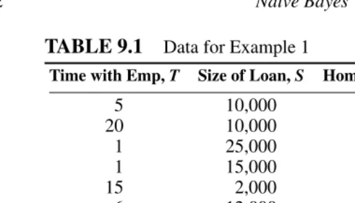
To illustrate the principles of the na¨ıve Bayes method, consider the artificial data set shown in Table 9.1. The aim is to use these data as a training set to construct a rule which will allow prediction of variable D for future customers, where D is default on a bank loan (the last column, labeled 1 for default and 0 for nondefault). The variables which will be used for the prediction are columns 1 to 3: time with current employer,
T , in years; size of loan requested, S, in dollars; and H , whether the applicant is a
TABLE 9.1
Data for Example 1Time with Emp, T Size of Loan, S Homeowner, H Default, D
5 10,000 1 0
20 10,000 1 0
1 25,000 1 0
1 15,000 3 0
15 2,000 2 0
6 12,000 1 0
1 5,000 2 1
12 8,000 2 1
3 10,000 1 1
1 5,000 3 1
Time with employer is a continuous variable. For each of the two classes separately,
we could estimate the distribution f (T|i ), i =0,1 using a kernel method or some
assumed parametric form (lognormal would probably be a sensible choice for such a variable), or we could use the na¨ıve Bayes approach in which the variable is split into cells, estimating the probability of falling in each cell by the proportion of cases from class i which fall in that cell. We shall take this third approach and, to keep things as simple as possible, will split T into only two cells, whether or not the customer has been with the employer for 10 or more years. This yields probability estimates
ˆf(T <10|D=0) = 4/6, ˆf(T ≥10|D=0)=2/6
ˆf(T <10|D=1) = 3/4, ˆf(T ≥10|D=1)=1/4
Similarly, we shall do the same sort of thing with size of loan, splitting it into just
two cells (purely for convenience of explanation) according to the intervals≤10,000
and>10,000. This yields probability estimates
ˆf(S≤10000|D=0) = 3/6, ˆf(S>10000|D=0)=3/6
ˆf(S≤10000|D=1) = 3/4, ˆf(S>10000|D=1)=1/4
For the nondefaulter class, the homeowner column yields three estimated proba-bilities:
ˆf(H =1|D=0)=4/6, ˆf(H =2|D=0)=1/6, ˆf(H =3|D=0)=1/6
For the defaulter class, the respective probabilities are
ˆf(H =1|D=1)=1/4, ˆf(H =2|D=1)=2/4, ˆf(H =3|D=1)=1/4
9.6 Examples 173
(T <10), is seeking a loan of $10,000 (S≤10000), and is a homeowner (H =1).
This leads to an estimated value of the ratio ˆP(1|x)/P(0ˆ |x) of
P(1|x)
P(0|x) =
P(1) P(0)
p
j=1 ˆf(xj|1)
ˆf(xj|0)
= P(1)
P(0)×
ˆf(T|1) ˆf (S|1) ˆf (H|1) ˆf(T|0) ˆf (S|0) ˆf (H|0)
= 4/106/10×4/63/4×4/6×3/4×3/6×1/4×4/6 =0.422
Since P(1|x)=1−P(0|x), this is equivalent to P(1|x)=0.296 and P(0|x)=0.703.
If the classification threshold is 0.5 [i.e., if we decide to classify a customer with
vector x to class 1 if P(1|x)>0.5 and to class 0 otherwise], then this customer will
be classified as likely to belong to class 0—the nondefaulter class. This customer would be a good bet for making a loan to.
9.6.2
Example 2
An important and relatively new application domain for the na¨ıve Bayes method is spam filtering. Spams are unsolicited and typically unwanted emails, often direct marketing of some kind and frequently offering dubious financial or other oppor-tunities. Some of them are so-called phishing exercises. The principle behind them is that even a low response rate is profitable if (a) the cost of mailing the emails is negligible and (b) enough are sent. Since they are sent out automatically to millions of email addresses, one may receive many hundreds of these daily. With this num-ber, even to move the cursor and physically hit the delete button would consume significant amounts of time. For this reason researchers have developed classification rules called spam filters, which examine incoming emails, and assign them to spam or not-spam classes. Those assigned to the spam class can be deleted automatically, or sent to a holding file for later examination, or treated in any other way deemed appropriate.
Na¨ıve Bayes models are very popular for use as spam filters, going back to the early seminal work by Sahami et al. (1998). In their simplest form, the variables in the model are binary variables corresponding to the presence or absence, in the email, of each word. However, the na¨ıve Bayes model also permits the ready addition of other binary variables corresponding to the presence or absence of other syntactic features
such as punctuation marks, currency units ($, £,€, and so on), combinations of words,
whether the source of the email was an individual or a list, and so on. In addition, other nonbinary variables are useful as further predictors, for example, the type of domain of the source, the percentage of nonalphanumeric characters in the subject heading, and so on. It will be clear from the above that the potential number of variables is very large. Because of this, a feature selection step is typically undertaken (recall the discussion of why the na¨ıve Bayes model may do well, despite its underlying independence assumption).
determining the classification threshold. In their experiments, Sahami et al. (1998)
chose a threshold of 0.999 with which to compare P(spam|x).
One strength of the na¨ıve Bayes model is that it can just as easily be applied to count variables as to binary variables. The multivariate binary spam filter described above is easy to extend to more elaborate models for the distributions of the values of the variables. We have already referred to the use of multinomial models ear-lier, in which continuous variables are partitioned into more than two cells (and the homeowner variable in the artificial data of Example 1 was a case of a trinomial variable). Experiments suggest that, at least for spam filtering, the multinomial ap-proach using frequencies of word appearances in the emails is superior to using mere presence/absence variables. Metsis et al. (2006) carried out a comparative analysis of different versions of the na¨ıve Bayes model, in which the marginal variables are treated in different ways, applying the methods to some real email data sets.
9.7
Advanced Topics
The chief attraction of the na¨ıve Bayes model is its extreme simplicity, permitting easy (univariate) estimation and straightforward interpretation via the weights of evidence. The first of these properties is also associated with robustness, provided the estimates of the marginal distributions are robust. In particular, if the marginal distributions are categorical, then each cell needs to contain sufficient data points to yield accurate estimates. With this in mind, researchers have explored optimal partitioning of each variable. The approach, most in tune with the straightforward na¨ıve Bayes estimator, is to examine each variable separately—perhaps splitting into equal quantiles (this is generally superior to splitting into equal length cells). A more sophisticated approach will choose the cells based on the relative number from each class in each cell. This can also be done by considering each variable separately. Finally, one can partition each cell taking into account the overall fit to the distribution in each (or both) classes, but this moves away from the simple marginal approach. Investigations of some of these issues are described in Hand and Adams (2000).
Missing data are a potential problem in all data analysis. Classification methods which cannot handle incomplete data are at a disadvantage. When the data are missing completely at random, then the na¨ıve Bayes model copes without any difficulty: Valid estimates are obtained by simply estimating the marginal distributions from the observed data. If the data are informatively missing, however, then more complex procedures are needed. This is an area meriting further research.
More and more problems involve dynamic data, and data sets which sequentially accrue. The na¨ıve Bayes method can be adapted very readily to such problems, by virtue of its straightforward estimation.
9.8 Exercises 175
much larger than the sample size. Such problems pose difficulties; for example, the covariance matrix will be singular, leading to overfitting. To tackle such problems, it is necessary to make some kinds of assumptions or (equivalently) to shrink the estimators in some way. One approach to such problems in the context of supervised classification is to use the na¨ıve Bayes method. This has its in-built assumption of independence, which acts to protect against overfitting. More elaborate versions of this idea combine na¨ıve Bayes models with more sophisticated classifiers, trying to strike the best balance.
9.8
Exercises
1. Using a package such as the open-source package R, generate samples of size 100 from each of the two classes. Class 1 is bivariate normal, with zero means and identity covariance matrix. Class 2 is bivariate normal, with mean vector (0, 2) and diagonal covariance matrix with leading diagonal (1, 2). Fit a na¨ıve Bayes model to these data, based on assuming (correctly) that the marginal distributions are normal. Plot the decision surface to see that it is not linear. 2. The tables below show the bivariate distributions from samples for two classes,
where the variables each have three categories. Show that the two variables are independent in each of the two classes. Taking the classification threshold as 1/2, calculate the decision surface for a na¨ıve Bayes classifier and show that it is nonlinear.
144 144 144
144 144 144
144 144 144
9 90 9
90 900 90
9 90 9
3. For the data from Exercise 2, calculate the weights of evidence for the categories of each variable, so that the na¨ıve Bayes classifier can be expressed as a weighted sum.
4. The tables below show the bivariate distributions from samples for two classes, where the variables each have three categories. Show that the two variables are
not independent in each of the two classes. Taking the classification threshold
27 30 27
30 2700 30
27 30 27
432 48 432
48 432 48
432 48 432
5. Using data simulated from multivariate normal distributions, compare the rel-ative performance of a na¨ıve Bayes classifier and a simple linear discriminant classification rule as the (assumed common) correlation between the variables increases.
6. Using a suitable data set from the UCI Machine Learning Repository, with continuous variables which are partitioned into discrete cells, investigate the effect of changing the number and width of the cells in each variable.
7. Using the same data set as in Exercise 6, compare the models produced by the na¨ıve Bayes classifier and logistic regression.
8. A common way to extend the na¨ıve Bayes classifier in some applications is to partition the data into segments, with separate na¨ıve Bayes classifiers con-structed for each segment. Clearly such partitioning will be most effective if its splits allow for interactions which the na¨ıve Bayes classifier would not pick up. Develop guidelines to assist people in making such splits.
9. The idea of modeling the distribution of each class by assuming independence extends immediately to more than two classes. For more than two classes write down appropriate classification models in the weights of evidence format. 10. One of the particular attractions of the na¨ıve Bayes classifier is that it permits
very simple estimation. Develop updating rules which allow the classifier to be sequentially updated as new data arrive.
References
Collett D. (1991) Modelling Binary Data. London: Chapman and Hall.
Domingos P. and Pazzani M. (1997) On the optimality of the simple Bayesian classifier under zero-one loss. Machine Learning, 29, 103–130.
Hand D.J. and Adams N.M. (2000) Defining attributes for scorecard construction.
References 177
Hand D.J. and Yu K. (2001) Idiot’s Bayes—not so stupid after all? International
Statistical Review, 69, 385–398.
Hastie T.J. and Tibshirani R.J. (1990) Generalized Additive Models. London: Chapman and Hall.
Jamain A. and Hand D.J. (2005) The na¨ıve Bayes mystery: A statistical detective story. Pattern Recognition Letters, 26, 1752–1760.
Jamain A. and Hand D.J. (2008) Mining supervised classification performance studies: A meta-analytic investigation. Journal of Classification, 25, 87–112.
Langley P. (1993) Induction of recursive Bayesian classifiers. Proceedings of the
Eighth European Conference on Machine Learning, Vienna, Austria:
Springer-Verlag, 153–164.
Mani S., Pazzani M.J., and West J. (1997) Knowledge discovery from a breast cancer database. Lecture Notes in Artificial Intelligence, 1211, 130–133.
Metsis V., Androutsopoulos I., and Paliouras G. (2006) Spam filtering with na¨ıve Bayes—which na¨ıve Bayes? CEAS 2006—Third Conference on Email and
Anti-Spam, Mountain View, California.
Sahami M., Dumains S., Heckerman D., and Horvitz E. (1998) A Bayesian approach to filtering junk e-mail. In Learning for Text Categorization—Papers from the AAAI
Workshop, Madison, Wisconsin, pp. 55–62.
Titterington D.M., Murray G.D., Murray L.S., Spiegelhalter D.J., Skene A.M., Habbema J.D.F., and Gelpke G.J. (1981) Comparison of discrimination techniques applied to a complex data set of head injured patients. Journal of the Royal