Primary User Avoidance algorithm for CRAHNs using Reinforcement Learning

International Journal of Innovative Technology and Exploring Engineering (IJITEE) ISSN: 2278-3075, Volume-8 Issue-11, September 2019



Abstract: Cognitive Radio Ad Hoc Networks (CRAHNs) are the need of the current time. There is a requirement of providing accessibility of network “everywhere”. This “everywhere” connectivity to all kinds of unlicensed devices is very hard to achieve in statically allocated spectrum bands. So CRAHNs were envisioned. In CRAHNs, it is very important to protect transmission of primary user. This paper tries to handle this concern. A reinforcement learning based algorithm is proposed and implemented which protects the transmission of primary user by avoiding secondary users to enter primary user coverage area, which is not known in advance. This algorithm will learn from its experience & once it has learnt from its environment, it always tries to avoid primary user within a region where primary user is operating on same channel as secondary user. This work includes Q learning along with neural networks (implemented in python). The experimentations results proved that this algorithm learns over time, because as the number of epochs are increased loss rate tends to decline. The algorithm is executed using neural networks with varying schemes. All of them proved that there is worthy amount of learning with decent accuracy. Results drawn from the proposed algorithm yield as output the distance covered by secondary user in each configuration, without hitting primary user and the mean loss rate for each configuration. The algorithm proposed in this paper is anticipated to be durable and robust. Moreover, it can work on large networks as well.

Keywords:CRAHNs, reinforcement learning, neural network, Q learning

I. INTRODUCTION OF CRAHNs

Spectrum is a valuable resource; spectrum assignment policy has divided it into licensed and unlicensed portions. Unlicensed portions are encumbered with massive number of users in current time and licensed portions are underutilized [1]. Keeping this into mind, Federal Communication Commission (FCC) has allowed unlicensed band radio devices to operate in licensed band on one condition: the unlicensed band users are allowed to use the licensed spectrum only when licensed users are not using it. However licensed users can use it anytime they want. Then unlicensed user need to vacate that band at that particular time & look for some other vacant spectrum.

Cognitive Radio Network (CRN) is this distinctive sort of network that utilizes the underutilized portion of statically allocated spectrum. Cognitive Radio Ad Hoc Networks (CRAHNs) are special sort of CRN which do not have any

Revised Manuscript Received on September2, 2019.

Shiraz Khurana*, Department of Computer Science & Applications,

Kurukshetra University, Kurukshetra, Haryana, India. Email:

[email protected]

Dr. Shuchita Upadhyaya, Department of Computer Science & Applications, Kurukshetra University, Kurukshetra, Haryana, India. Email: [email protected]

infrastructural support (like base station etc.). It is a distributed network with additional capabilities and constraints than classical ad hoc networks. In CRAHNs the unlicensed users are considered as Secondary Users (SUs) while the licensed users will be termed as Primary Users (PUs).

SUs will look for vacant spectrum areas identified as spectrum holes. If PUs desire to use any of these spectrum holes, they can use it any time and at that time SUs will look for another vacant spectrum hole to continue their communication. There is an alternative solution also: SU may reduce its transmission power to such an extent that it will not disturb PU’s transmission.

The target in this paper is that SU should not enter the area in which PU is operating on the same channel. Some of the existing literature assumes that PUs transmitters will share their future spectrum usage pattern in advance which is very tough in real implementation, SU must be smart enough to avoid that geographical area in which PU is operating on the same channel.

Machine learning is the current need of the day for achieving smart decisions. In this paper one specific branch of machine learning known as reinforcement learning has been exploited. This learning will be used to avoid PUs operating areas. This paper proposes and implements a reinforcement learning based algorithm which protects the transmission of PUs by avoiding SUs to enter PUs coverage areas, which is not known in advance. This algorithm will learn from its experiences & once it has learnt from its environment, it always tries to avoid PUs within a region where PU is operating on same channel as SU. This work includes Q learning along with neural networks (implemented in python). Following this introductory section. This paper is divided into 8 sections. In section II, the role & components of an agent are discussed. Section III gives an introduction to reinforcement learning. In section IV, existing work on reinforcement learning in cognitive radio ad hoc network is described. Section V describes an introduction to neural networks. In Section VI, Q learning algorithm has been proposed and developed by using neural networks. In section VII, the experimentation performed & its outcomes are described. Section VIII elucidates the conclusions.

Primary User Avoidance algorithm for CRAHNs

using Reinforcement Learning

II. ROLE OF AN AGENT

An agent is one that can view or perceive its environment through its sensors and act upon its environment through actuators. An agent, will have 4 major properties attached to it: Performance, Environment, Actuators and Sensors, jointly known as PEAS. Table 1 shows the PEAS table for an agent whose task it to avoid hitting PU region and make sure that it operates within a bounded geographical area.

Table 1: PEAS table for the agent

Performance Environment Actuators Sensors

Not hitting to Primary User area, More distance travelled by SU.

Grid boundary, Primary User

Motion Sensors

Spectrum Observing Sensors

The components of agent are described as in figure 1. Agent will observe the percept from the environment and based on internal configuration, takes some action through its actuators.

Figure 1: Components of an agent

III. REINFORCEMENT LEARNING

Reinforcement Learning (RL) is a branch of machine learning (ML) which allows an agent to take specific action in current state & the resulting state will be examined as “good” or “bad” state. In the absence of pre-existing data, the training of an agent will be a tedious task which can be done by using reinforcement learning. An agent can take action in environment but without any feedback there is no way agent can tell what is good and what is bad. It needs some sort of feedback called as reinforcement or reward (R). So reinforcement learning is a feedback based learning. If it is “good” state, the probability of taking same action in same situations will be amplified for future. In other words R is positive. But if the resulting state is observed as “bad” state, then probability of taking the same action in the same situation will be lessened for future. So R can be considered as negative. RL is designed to observe rewards & to learn an optimal policy for the environment. The agent life cycle of working is depicted in Figure 2. St and St+1 are the current state & next state respectively, Rt and Rt+1 are the rewards for current state & next state respectively and At is the action.

Figure 2: Agent Life cycle in reinforcement Learning

IV. REINFORCEMENT LEARNING IN CRAHNs

In this section literature relevant to the usage of reinforcement learning in CRAHNs is described. The literature described pertains to learning & routing in CRAHNs.

In [2] Khurana et al. proposed a combination of RL & CRAHNs. Further Q learning algorithm & Q function have been used to update rewards. The distinguishing features of this algorithm are;

 It can be used to avoid PU on different channels after a nominal training & once the model is trained properly (in 8 epoch approximately). The chances of hitting PU is almost zero, if there is any change in the network, then based on the change re-learning will occur.

 The algorithm is faster in learning process when operated on small networks.

Tables has been used for storing the current state, action, new state, reward and Q value. If there is small change in position of PU managing tables will be cumbersome as all the tables need to be replaced.

In [3] Aqueel et al. proposed three different routing schemes out of which two are based on Reinforcement Learning (RL) concept and one is based on Spectrum Leasing (SL) concept. The main difference between SL and RL is: In SL secondary user will receive information about the activity area of PU in advance, called as spectrum occupancy map. The source node will select its neighbor for a specific route between source and destination which offers the highest minimum channel available time. RL based technique do not have any spectrum occupancy map in advance. One algorithm does it by using traditional RL based scheme while another calculates average Q value. It selects a route which has been selected for transmission in the past maximum number of times. The experimentation has been performed on two different types of topologies, a 6 node network and a 10 node network. Evaluation is performed on real testbed using software radio peripheral and GNU radio units. The protocol has been compared with exiting work in the literature & superiority of the work has been proved in terms of route selection, throughput and packet delivery ratio.

In [4] Cheng et al. proposed an approach that improves spectrum management by using multi-agent reinforcement learning. It further considers a function to determine the precedence of different channels & frequency bands.

Kanerva based function has been employed to evaluate and improve the accuracy of the model. The main purpose of the approach is to reduce the interference to the licensed users. It is shown that in comparison to random or greedy approaches, reinforcement learning reduces the chances of hitting Primary User.

V. NEURAL NETWORK

International Journal of Innovative Technology and Exploring Engineering (IJITEE) ISSN: 2278-3075, Volume-8 Issue-11, September 2019

calculation based on weight parameter & bias and then pass it to activation function to produce the output. The weight parameter represents the strength of connection between two neurons. The bias parameter is considered as an extra input to neuron, which is always ON & has its own value. The purpose of activation function is to make unbounded input to a measurable and bounded form. There are a variety of activation functions available in literature [5]. ReLU (Rectified Linear Unit) [6] has been used in the present proposed work since it can fix vanishing gradient problem.

An example of a neural network is shown in figure 3. The leftmost layer is the input layer, and the rightmost layer is the output layer. The middle layer, which can be more than one, is the hidden layer/s.

Figure 3: Sample Neural Network

The number of neuron in input & output layers depends specifically on the problem statement. The number of input parameters will determine the neurons in input layer and the output required from the model will determine the number of neurons in output layer. The number of neurons in hidden layer is based on some heuristics, there is no specific rule for this; for experimentation many combinations are tried. The number of neurons in hidden layer are taken according to the best result obtained.

VI. Q LEARNING USING NEURAL NETWORK

In this section, the Q learning algorithm is described in detail. A code has been developed in Python to implement it. Concept of learning has been described first. Then symbols and terms used in the algorithm are discussed. At the end of this section proposed algorithm is explained.

A.Learning

In machine learning, learning refers to the ability to remember some environment status, so that if the same kind of scenario reoccurs, same or better action can be executed. A set of symbols have been used in the algorithm. Table 2 gives the naming of these symbols.

Table 2: Description of symbols used in Algorithm

Name of Variable Symbol used

Epsilon: ϵ

Epoch (number of iteration): α

Epoch (Maximum number of iteration):

αmax

Epoch (number of observed

iteration):

αobser

Batch size: Bsize

Present State of SU: Scurr

Old State of SU: Sold

New State of SU: Snew

Reward: R

Non-terminal state (not hitting PU): Snon-term

Terminal state (hit PU): Sterm

Gamma (discount factor): γ

Random: Rand

In proposed model before the actual learning starts, the environment is observed for some time. The sensing module of SU will send the current state of the system. Based on this state, Q values will be predicted. Three different actions can be taken: moving SU towards left side, right side, or straight. Out of these actions, which ever has the maximum Q value will lead to the execution of that action. For the first time, Q value is same for all actions. Hence in the beginning observations are performed so that the model will have something to start with. Then a random number is generated. If it is less than epsilon (ϵ), random action is selected for execution. If it is higher than ϵ, then most confident action is returned from the prediction. The ϵ value will vary between 0 & 1, initially the value of ϵ as 1 so that the action will be totally random in the beginning & value is decreased continuously. Consequently, after learning, the action will be based on prediction, not on random basis. In other words, the model performs exploration in the beginning & later it does exploitation of the solution domain. Then based on choice, the action is taken, the next value is observed, the reward received. These values are stored in some list. The values are processed in the form of batches, not in a single value manner so that better performance is obtained. These steps are repeated until the epoch is not greater than predefined observed value of epoch.

Now fetch a random sample from the list which contains; old state, action taken, reward received & new state; then learning is carried out by building input & output sets. The following is the proposed algorithm.

A.Algorithm for training the Model:

Step 1: Initialize parameters; ϵ, α, Bsize.

Step 2: Read the Scurr of SU from the grid created & return R (for first time it is random).

Step 3: if α < αmax then keep repeating for training // this will be repeated till the end

Step 4: Generate random number, if (Rand < ϵ) or (α < αobser): Rand action (left, right, straight). Else: execute action [max Q value [action]].

Step 5: List L= L+ (Sold + Snew + action + R)

Step 6: if (α > αobser) then repeat: Sample S= Rand (L). Step 7: if (R=-100): Snew = Sterm & keep the reward same. Else:

Snew = Snon-term & R= R + γ* max (Q value). Store this value

pair again as training input and output.

Step 8: Fit the model & check for loss function.

If reward is -100 then record the distance SU has travelled along with the loss occurred. Jump to step 2.

Step 9: Repeat until desired number of epochs are over. Reduce the ϵ value at a constant rate.

B.Explanation of Algorithm:

or to take what the model believes to be the best action available at any time. To do this, a random value is generated. If it is greater than ϵ, then it will withdraw the value from the learning model and takes the action based on maximum Q value. The actions are recorded as left, right or straight. The value for Epoch (α) is considered as number of iterations the algorithm will cover. “Larger the Better” is the principle of epoch but it comes with more resource consumption. So it has to be balanced between accuracy and resource consumption. One more parameter named batch size (Bsize) is taken. The processing of all input & output in terms of sets is called batches. In case single observation is taken at a time it will go through various steps which obviously takes lots of learning time & difficult to manipulate. In step 2 the current state of the grid is being monitored where SU and PUs are placed in different positions. It will be recorded in which position SU is operating & what rewards it receives after reaching to this state. In initial state, it has a default value, then it starts to get trained, till α < αobser. When it is in observing state, all its actions are random & it will record the value of environment in this step, so that it will have something to start with. Once it is done with observation part, it means now the value of α > αobser. Now it will be recording Sold,R, action & Snew. Now it is time to compute Q value for each action that possibly it is going to take. More the Q value for an action, superfluous are the chances of taking that action. Once action is taken, it will record new state and reward. The proposed algorithm also assumes that in case it tries to learn more than the space allocated for learning, it will be replacing the oldest entry from the memory with the new one. It will repeat this process continuously until the number of epochs reaches to αmax. While recording the rewards, it will also record the distance travelled by SU without hitting the PUs in each epoch, and the number of times it hit PUs so that it will be able to measure the loss rate at the end of the training.

VII.EXPERIMENT & RESULTS

The motive of this experimentation is to prove that the agent has learnt from its environment over time. This can be verified by checking the distance travelled by SU without hitting PUs. It also monitors a loss function which will show the reward it has received over time and more the rewards, less will be the loss.

Table 3: Experimentation parameters

Parameter Name Parameter Value

Size of the grid 1000*1000

Number of SU 1

Number of PU 2

Number of Channels 2

Input layer number of neurons 2, 128, 256

Hidden layer number of neurons 128,256

Output layer number of neurons 3

Activation function ReLU (input), ReLU (hidden layer),

Linear (output layer)

Dropout value 0.2

Optimizer ADAM (adaptive moment

estimation)

This loss function should gradually reduce over time only then it will be able to consider that this algorithm has learnt something. In Table 3, the parameter values used in this experiment are mentioned.

A grid of 1000 * 1000 is created using Pygame libraries in Python [7], in which 2 primary users (PUs) & 1 Secondary user (SU) are created. There are 2 licensed channels allocated one to each PU. They are dedicatedly operating on that channel only. The SU may work on any of these channels, but not at same time & location where PU is active. Outside PU’s region, SU is allowed to use the same channel without causing any hindrance to PU’s transmission. The range of PU is three times more than SU.

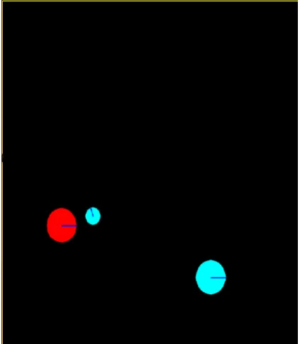
The PU’s activities are modeled according to exponential distribution, to show ON & OFF nature of PUs. From the grid the position, reward & action values are observed continuously. In Figure 4, both the PUs are active at the same time (two bigger balls). SU is operating on channel number 2 (shown with the help of small circle) near PU which is operating on different channel (shown with the help of different color).

International Journal of Innovative Technology and Exploring Engineering (IJITEE) ISSN: 2278-3075, Volume-8 Issue-11, September 2019

Figure 5: one PU is active and other is inactive In Figure 5, one of the PU is active (one is shown in red color which is active & another in grey color to show that it is inactive). SU is operating on channel number 2 near PU which is operating on different channel (shown with the help of different colors).

Further, a neural network model is created with the following configuration: Keras model libraries are used which are available for open access in Python. A sequential model with three layers is formed: the first layer is input layer which has 2 neurons, second layer is hidden layer which has 128 neurons and third layer is output layer which has 3 neurons. The activation function ReLU is used at both input and hidden layer while linear activation function is used at the output layer. Dropout value is taken as 0.2 to prevent overfitting of the proposed model. ADAM (adaptive moment estimation) optimizer is used to update weights to minimize the value of loss function. ADAM function is considered as combination of AdaGrad and RMSprop since it combines the best properties of both of these optimizers.

A. Results

After execution, the following results are observed:

This model is executed with three different neural network configurations;

 The first configuration has: 2 neurons for the input layer, 128 neurons for the hidden layer, and 3 neurons for the output layer).

 The second configuration (128 neurons for the input layer, 128 neurons for the hidden layer and 3 neurons for the output layer).

 The third configuration (256 neurons for the input layer, 256 neurons for the hidden layer, 3 neurons for the output layer).

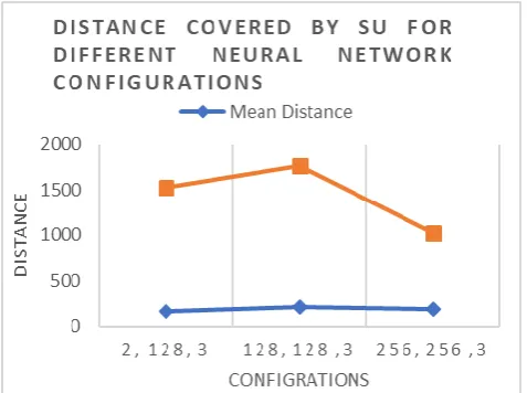
Figure 6 shows the maximum distance covered by SU without hitting PU for each configuration. The mean distance is the mean of all the distance covered by SU in particular neural network configuration.

Figure 6: Maximum and Mean distance covered by SU From Figure 6, we can conclude that the maximum & mean distance values for the SU in configuration (128 neurons for the input layer, 128 neurons for the hidden layer and 3 neurons for the output layer) is best among all the three configurations.

Figure 7, shows the minimum loss incurred by SU for each configuration. The mean loss is the mean of all the loss incurred by SU in particular neural network configuration.

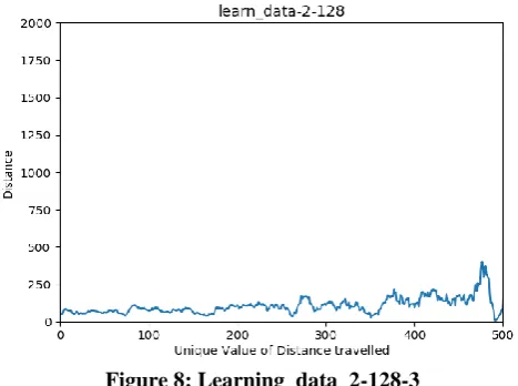
Figure 8: Learning_data_2-128-3

Figure 9 shows the learning data of distance travelled by SU for neural network (128 neurons for the input layer, 128 neurons for the hidden layer, and 3 neurons for the output layer).

Figure 9: Learning_data_128-128-3

Figure 10 shows the learning data of distance travelled by SU for neural network (256 neurons for the input layer, 256 neurons for the hidden layer, and 3 neurons for the output layer).

Figure 10: Learning_data_128-128-3 For individual learning shown in Figure 8, 9 & 10: we can conclude that in Figure 8, for the 1st configuration the variance in distance coverage by SU is high as the number of neurons in input layer are 2 only. In figure 9, 2nd configuration is shown: in this the variance is a bit less than the 1st configuration, but the distance covered by SU without hitting

PU takes highest values, amongst all three configurations. In Figure 10, the third configuration (256 neurons for the input layer, 256 neurons for the hidden layer, and 3 neurons for the output layer) shows least variance in distance coverage, but the distance covered is also less than 2nd configuration. So, distance coverage for the 2nd Configuration is best.

Figure 11 shows the loss incurred by SU for neural network (2 neuron for input layer, 128 neuron for hidden layer, 3 neuron for output layer). The loss incurred is continuously decreasing so it can be concluded that this model has learnt.

Figure 11: Loss incurred by SU over 100000 Epoch Figure 12 shows the loss incurred by SU for neural network (128 neurons for input layer, 128 neuron for hidden layer, 3 neuron for output layer). The loss incurred is continuously decreasing so it can be concluded that this model has learnt.

International Journal of Innovative Technology and Exploring Engineering (IJITEE) ISSN: 2278-3075, Volume-8 Issue-11, September 2019

Figure 13: Loss incurred by SU over 100000 Epoch The loss incurred by each of these configurations is shown in Figure 11, 12 & 13, which can be interpreted as follows: The 1st configuration has the highest loss rate followed by 2nd and 3rd configuration. The mean loss rate of 3rd configuration is 67 % less than 1st configuration and the mean loss rate of 2nd configuration is 59% less than 1st configuration. So from loss rate point of view, the 3rd configuration is the best.

VIII: CONCLUSION

In this paper a reinforcement based learning approach is proposed & implemented, especially when PUs are active. First, a discussion about Cognitive radio ad hoc networks is presented, then reinforcement learning & neural network have been discussed. Subsequently, Q learning algorithm (the code is developed in Python) is explained. The experimentation results proved that this algorithm developed has learnt over time. As number of epochs are increased, the loss rate tends to decline. The algorithm has been executed by using various neural network schemes. All of them proved that there is worthy amount of learning with decent accuracy. Results drawn from the proposed algorithm yield as output the distance covered by secondary user in each configuration, without hitting Primary User and the mean loss rate for each configuration. So it can be concluded that in case the priority is distance coverage, second configuration mentioned in the paper can be preferred, and if the loss rate is priority, then third configuration can be chosen. The algorithm proposed in this paper is anticipated to be durable and robust. Moreover it can work on large networks as well. The future work will be to extend this work in routing of Cognitive radio ad hoc network.

REFERENCES

1. Akyildiz IF, Lee WY, Chowdhury KR (2009) CRAHNs: cognitive radio

ad hoc networks. Ad Hoc Netw 7(5):810–836.

2. Khurana, Shiraz; Bhasin, Shuchita; "Spectrum Management in

Cognitive Radio Ad-Hoc Network Using Q- Learning", International Journal of Information Technology, Springer Singapore, ISSN: 2511-2104, PP (1-6). 2018

3. Syed, Aqeel Raza et al. “Route Selection for Multi-Hop Cognitive Radio

Networks Using Reinforcement Learning: An Experimental Study.” IEEE Access 4 (2016): 6304–6324. IEEE Access.

4. Wu, Cheng; Chowdhury, K., Felice, M. D., Pourpeighambar, B.,

Dehghan, M., & Sabaei, M. (2010). Spectrum Management of Cognitive Radio Using Multi-agent Reinforcement Learning Categories and Subject Descriptors. In Autonomous Agents and Multiagent Systems (Vol. 106, pp. 1705–1712).

5. Gupta, D. and Them, F. (2019). Fundamentals of Deep Learning -

Activation Functions and their use. [online] Analytics Vidhya. Available at:

https://www.analyticsvidhya.com/blog/2017/10/fundamentals-deep-learn ing-activation-functions-when-to-use-them/ [Accessed 30 Aug. 2019].

6. Brownlee, J. (2019). A Gentle Introduction to the Rectified Linear Unit

(ReLU). [online] Machine Learning Mastery. Available at:

https://machinelearningmastery.com/rectified-linear-activation-function-for-deep-learning-neural-networks/ [Accessed 30 Aug. 2019].

7. Harvey, M. (2019). Using reinforcement learning in Python to teach a virtual car to avoid obstacles. [online] Medium. Available at: https://blog.coast.ai/using-reinforcement-learning-in-python-to-teach-a-v irtual-car-to-avoid-obstacles-6e782cc7d4c6 [Accessed 30 Aug. 2019].

AUTHORSPROFILE

Dr. Shuchita Upadhyaya Bhasin working as a professor in Dept. of Computer Science & Applications, Kurukshetra University. She is having more than 31 years of teaching experience. She has been Awarded Kunj Ratan, Award of Honour, for exemplary achievement in the field of academics by Haryana Government. Her Specialization and areas of interest includes: Computer Networks and Data Communication, Internet Technologies, Wireless Technologies, Wireless Sensor Networks, Ad-hoc Networks, Network Security, Soft Computing, Data Mining & Computer Graphics. She has guided more than 12 Ph.D students. She has published more than 100 International/National journal papers and two books as well. She has attended more than 100 conference and seminars. She has authored more than 150 lessons for correspondence courses run by the Dept. of Distance Education, Kurukshetra University.