Topics in hyperbolic groups

warwick.ac.uk/lib-publications

A Thesis Submitted for the Degree of PhD at the University of Warwick

Permanent WRAP URL:

http://wrap.warwick.ac.uk/110993

Copyright and reuse:

This thesis is made available online and is protected by original copyright.

Please scroll down to view the document itself.

Please refer to the repository record for this item for information to help you to cite it.

Our policy information is available from the repository home page.

BRITISH THESIS SERVICE

COPYRIGHT

Reproduction of this thesis, other than as permitted under

the United Kingdom Copyright Designs and Patents Act

1988, or under specific agreement with the copyright

holder, is prohibited.

This copy has been supplied on the understanding that it

is copyright material and that no quotation from the thesis

may be published without proper acknowledgement.

REPRODUCTION QUALITY NOTICE

The quality of this reproduction is dependent upon the

quality of the original thesis. Whilst every effort has been

made to ensure the highest quality of reproduction, some

pages which contain small or poor printing may not

reproduce well.

Previously copyrighted material (journal articles, published

texts etc.) is not reproduced.

Topics in Hyperbolic Groups

Stephen Billington

Thesis submitted for the degree of PhD at the Mathematics Institute, University o f Warwick

1 B a c k g r o u n d 8

1.1 Hyperbolic G r o u p s ... 9

1.1.1 Definitions of H y p e r b o lic ity ... 9

1.1.2 The Boundary o f a Hyperbolic G r o u p ... 13

1.2 Autom atic G r o u p s ... 18

1.2.1 Finite State A u t o m a t a ... 18

1.2.2 Automatic G r o u p s ... 19

1.2.3 Hyperbolic G r o u p s ... 20

1.3 Computability Problems in G r o u p s ... 21

1.3.1 Computability in Hyperbolic g ro u p s... 22

1.3.2 Unsolvable Problems in Hyperbolic G rou p s... 25

2 C o m p u t in g th e H o m o lo g y o f a H y p e r b o lic G ro u p 27 2.1 Constructing a Contractible Space with Rigid G-action, Finite Stabilisers and Finite Q u otien t... 28

2.2 Constructing a Contractible Space with a Free G-action and Finite Quotient in Each D im e n s io n ... 30

2.2.1 Simplicial Cell Complexes o f G r o u p s ... 31

2.2.2 Returning to our S itu a tio n ... 33

2.2.3 The Fundamental Group of a Complex o f Groups . . . 34

2.2.4 Categories and Classifying S p a c e s ... 34

2.3 Examples ... 40

3 T h e B o u n d a r y o f a H y p e r b o lic G r o u p as an In verse L im it o f F in ite S e ts 49 3.1 The Boundary as an Inverse L im it... 50

3.1.1 Constructing Finite Topological S p a c e s ...50

3.1.2 The Restriction M a p ... 52

3.1.3 The Inverse L im it... 53

3.1.4 Hausdorffifying the Inverse L i m i t ... 56

3.1.5 The Topology of H ... 57

3.2 Similar Constructions... 64

3.3 A p p lica tion s... 67

CONTENTS 3

4 S y m b o lic D yn am ics in H y p e r b o lic G r o u p s 74

4.1 Symbolic D y n a m ics... 75

4.1.1 Subshifts o f Finite Type Over a G r o u p ...75

4.1.2 Dynamical S y s te m s ... 76

4.1.3 Examples o f Subshifts o f Finite Type Over Z ... 77

4.1.4 Finitely Presented Dynamical S y s t e m s ...80

4.1.5 Semi-Markovian Spaces... 81

4.1.6 An Alternative G-Action on E(G, S ) ... 81

4.2 The Boundary o f a Hyperbolic Group as a Dynamical System 85 4.2.1 G e o d e s ic s ... 86

4.2.2 The Subshift <1>... 89

4.2.3 The Dynamical System (d G ,G ) is Finitely Presented . 99 4.2.4 An Instructive E x a m p l e ...103

4.3 The Boundary as a Semi-Markovian S p a c e ...105

4.4 The Geodesic F l o w ... 107

5 C a y ley G rap h s w h ich a re R egu la r T ilin g s 114 5.1 Introduction... 115

5.2 Platonic Solids ... 116

5.2.1 The T e tr a h e d r o n ... 117

5.2.2 The C u b e ... 117

5.2.3 The O ctah edron ... 121

5.2.4 Relator t y p e s ...123

5.2.5 The D o d e ca h e d ro n ... 126

5.2.6 The Icosahedron ... 127

5.3 Regular T ilin g s ... 130

5.3.1 Regular Tilings Which are not Cayley G r a p h s ... 130

5.3.2 The Case W hen s is E v e n ...131

5.3.3 The Block C o n s tr u c tio n ...132

5.4.4 The Case W hen s is O d d ...142

5.3.5 Some Other E x a m p le s ... 142

5.4 O rbifolds... 145

5.4.1 The Orbifold Associated to E (s, v ) ...146

5.4.2 The Orbifold Associated to B ( s , v , d ) ... 146

5.4.3 The Orbifold Associated to D (p v ,v) ... 150

5.4.4 The Orbifold Associated to F ( s , 2 s ) ...150

5.5 Semi-Regular T i l i n g s ...152

5.5.1 Archimedean S o lid s ... 153

1.1 Thin trian gles... 1.2 Slim tria n g le s ... 1.3 The minsize of a tria n gle... 1.4 Geodesics which d i v e r g e ... 1.5 The visual metric on d r ... 2.1 The conjugator ga,b = g~±g~lgp,T ... 2.2 The relationships between the different categories here and in

[Hae92]... 2.3 The Rips complex o f Z :) ... 2.4 Choosing representatives in each orbit ... 2.5 The 1-skeleton o f B (Z 3) ... 2.6 Part of the tiling by (7r /2, 7t/ 3 , 7r /7)-triangles... 2.7 The quotient space for the (n/2,7r /3,7r /7)-triangle tiling under

the action of the (2,3,7)-triangle g r o u p ... 2.8 Labelling edges and finding con jugators... 2.9 Labelling the f a c e s ... 2.10 The 1-skeleton o f the quotient space G \B G C for the (2 ,3 ,7

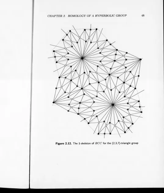
)-triangle group... 2.11 The 1-skeleton o f B G C for the (2,3,7)-triangle g r o u p ... 2.12 The 1-skeleton o f B C C for the (2,3,7)-triangle g r o u p ... 3.1 The relationship between F, W and S ... 3.2 F\, part, o f the Cayley graph and Si o f the fundamental group

o f a surface o f genus 2 ... 3.3 The restriction map /2 ... 3.4 A geodesic q u a d rila te ra l... 3.5 The set Zv as in the proof of Theorem 3 .1 .1 5 ... 3.6 The difference between Ym and Vm ... 3.7 S\ and 5js for Example 3 .2 .3 ... 3.8 Straightening out a stranded e d g e ... 3.9 Si, S2 and S3 o f F(a,b) x Z2... 3.10 S, and S2 o f n ,(T 2) * Z ... ! . . . 4.1 A cylinder in £ (Z , {a, b, c } ) ... 4.2 The cylinders for Example 4 .1 . 3 ... 4.3 Neighbouring states in a finite state a u t o m a t o n ...

C

l

C

l

LIST OF FIGURES 5

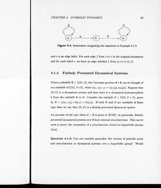
4.4 Automaton recognising the sequences in Example 4.1.5 . . . . 80

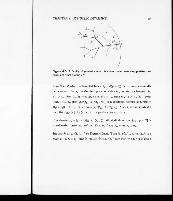
4.5 A family of geodesics which is closed under removing prefixes . 87 4.6 If h is in a g, then a/, is a suffix o f a g ...88

4.7 Words accepted by W D ( X ) ...92

4.8 The condition for 4>... 94

4.9 There is a </>- gradient from each vertex o f F... 97

4.10 Geodesics in WT>(X) through g and h ... 98

4.11 The condition on $ x 4> ... 102

4.12 The geodesic acceptor for the free group with 2 generators . . 104

4.13 Tracing a geodesic in F2 ...105

5.1 The choice of x determines the Cayley graph...121

5.2 The 1-skeleton o f the d odecah ed ron ... 127

5.3 The 1-skeleton o f the icosahedron... 128

5.4 4-gons meeting 6 to a v e r t e x ... 132

5.5 The d - b l o c k ...133

5.6 The (d — 1, l)- b lo c k ... 134

5.7 The (d + l ) - b l o c k ... 135

5.8 The (d + /c )-b lo ck ... 135

5.9 The (2 d + k)-b l o c k ... 136

5.10 The block d ia g r a m ... 137

5.11 The dual p o ly g o n ... 138

5.12 The side pairing for a generator x* o f order 2 ... 139

5.13 The side pairing o f a generator aj o f order s ...140

5.14 The side pairing o f an infinite order generator bjt\ ... 140

5.15 The side pairing for D (p v ,v )...143

5.16 The side pairing for F (s ,2 s ) where s is odd... 144

5.17 The relators for F (s,2 s ) where s is o d d ... 145

5.18 The block diagram r e v is it e d ... 147

5.19 A cone point o f order s ...148

5.20 A cone point o f order 2 ...149

5.21 The orbifold Q (B (s, v, d)) ... 149

5.22 Identifications to obtain Q ( F ( s , 2 s ) ) ... 151

5.23 The first piece o f Q (F (s ,2 s )) 151 5.24 The second piece o f Q (F (s, 2 s ) ) ... 152

5.25 The Archimedean s o l i d s ...154

5.26 An unflankcd 4 -b lo c k ... 155

.27 A quasi-regular tiling by squares and p e n ta g o n s ...159

1 The free group on 3 generators... 2 Z3* Z3 = (a, 6 | a3, ft3) ... 3 The fundamental group o f the torus o f genus 2 ... 4 Z4 = (a, 6 | a4, 6 = a2) ... 5 Z2 x Z2 = (a, 6, c | a2, 62, ab = 6a, c = a6) ...

6 Z4 x Z2 = (a, b | a4,62, ab - b a ) ... 7 D6 = (a, 6 | a4,62,(a6)2) ...

8 D8 = (a, 6, c | a2,62, (a6)4, e = 6a6) ... 9 Z2 x Z2 x Z2 = (a, 6, c | a2, 62, c2, ab = 6a, 6c = c6, ca = ac)

10 Z8 = (a, 6 | a8, 6 = a4) ...

11 Zg = (a, 6 | a6, 6 = a2) ...

12 D6 = (a ,b ,c \ a2,b2,(ab)3,c = ab) ...

13 A4 = (a, 6, c | a3,63, (a6)2, c = a6) ... 14 S4 = (a, 6 | a3,64,(a6)2) ...

Acknowledgements

First and foremost, I would like to thank my supervisor, David Epstein, for his guidance, inspiration and encyclopaedic knowledge of mathematics.

I would also especially like to thank Andrew Clow for countless useful conversations. Also, my thanks go to Caroline Series, Swarup Gadde, Giles Robert, Alison Kay, Charles Walkden, Timothy Luffingham and Rob Foord for their help and interest.

Declaration

Chapter 1 is expository. To the best o f my knowledge, the other chapters are original, except where stated. Some o f the results in Chapter 3 are being submitted for publication as part of a joint paper with David Epstein and Derek Holt. The results which appear in Chapter 3 are my ow n work.

Summary

Hyperbolic groups are a class of groups introduced by Gromov in 1987, which form an important part of geometric group theory. In Chapter 1, we give an introduction to this subject.

In Chapter 2, we use the theory o f complexes of groups to show that the integral homology and cohomology groups o f a hyperbolic group are computable by a Turing machine.

In Chapter 3, we present the boundary of a hyperbolic group as an inverse limit of topological spaces and use this to give computable estimates for properties o f the boundary.

In Chapter 4, we investigate symbolic dynamic properties concerning hy­ perbolic groups. In paricular, we give symbolic codings for the actions on the boundary of a hyperbolic and actions on the geodesic flow on a hyperbolic group.

In Chapter 5 we investigate the problem o f determining when graphs are Cayley graphs. The graphs which we are concerned with are regular and semi-regular planar graphs.

Background

Throughout this chapter, G is a finitely generated group with finite generat­ ing set X . A n element g o f G can be written as a product x,\ ■ • -x n, where each Xi is either in X or is the inverse of an element o f X . Such a product is called a representative o f g. The length of g (written |<?|) is the minimum number o f elements in a representative of g. We equip G with the word

metric, d(g, h) = \g - h\ = \g~lh\.

D efin ition 1.0.1 (C a y le y G r a p h ): The Cayley graph T(G, X ), or I when there is no ambiguity, is the graph with, for each g € G, a vertex labelled g and for each g 6 G, x G X an edge from g to g x labelled by x. We give I' a metric by giving each edge length 1 and then taking the path metric. This metric coincides with the word metric on the vertices of I . We use d(x, y) or

\x — y | to denote the distance between two points x, y 6 F.

D efin ition 1.0.2 (G e o d e s ic ): A geodesic in F is an isometric embedding of a closed interval into F. Suppose that 7 : [a, 6] —► F is a geodesic with

7(a) = x and 7(b) = y. We sometimes write [x, y] for 7.

CHAPTER 1. BACKGROUND 9

1.1

Hyperbolic Groups

Hyperbolic groups are a class o f groups introduced by Gromov in [Gro87] whose Cayley graph satisfies a single axiom (see Definition 1.1.2). Hyper- bolicity is independent o f the choice of finite generating set. The definition applies to more general spaces than Cayley graphs and gives rise to the no­ tion o f a hyperbolic space. For simplicity, we stick to the case of a Cayley graph.

Good introductions to the theory o f hyperbolic spaces and hyperbolic groups are [ABC+91], [CDP90] and [GdlH90], All the information in this section has been taken from these books.

1.1.1

D efinitions o f H yperholicity

D e fin itio n 1.1.1 (In n er p ro d u ct [G ro8 7]): Fix a basepoint x0 in T. For any two points x, y € F, define the inner product

D e fin itio n 1.1.2 (H y p e r b o lic [G ro8 7 ]): The group G with generating set

X is ¿-hyperbolic if, for any three points x, y, z € F,

(X V) = - (d (x0, i ) + d (x „,y ) - d ( x , y ) ) . (1.1)

(x.z) ^ min((x.j/), (y.z)) - 6. (1.2)

x2

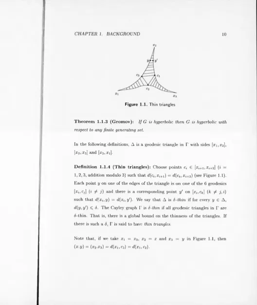
Figure 1.1. Thin triangles

T h e o r e m 1.1.3 (G r o m o v ): If G is hyperbolic then G is hyperbolic with

respect to any finite generating set.

In the following definitions, A is a geodesic triangle in T with sides [x i,x 2], [x2,x 3] and [x3, Xi].

D e fin itio n 1.1.4 (T h in trian gles): Choose points c* G [x1+i ,x i+2] (i = 1 ,2,3, addition modulo 3) such that d(ci,xi+1) = d (c i,x i+2) (see Figure 1.1). Each point y on one of the edges o f the triangle is on one of the 6 geodesics

[xi,Cj\ (i / j ) and there is a corresponding point y' on [x,, c*] (k ^ j, i)

such that d (x i,y ) = d(xi,y'). We say that A is S-thin if for every y G A,

d (y,y') < <5. The Cayley graph T is S-thin if all geodesic triangles in T are

¿-thin. That is, there is a global bound on the thinness of the triangles. If there is such a 6, T is said to have thin triangles.

Note that, if we take x t = xq, x2 = x and X3 = y in Figure 1.1, then

CHAPTER 1. BACKGROUND 11

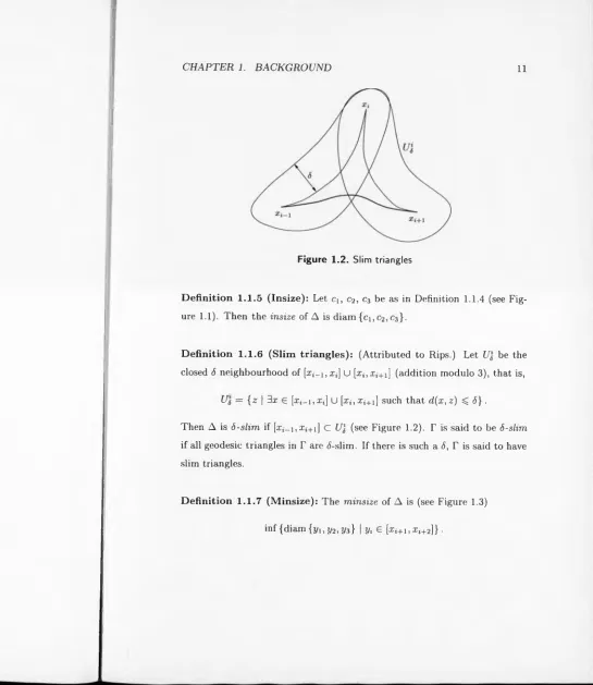
Figure 1.2. Slim triangles

D e fin itio n 1 .1 .5 (In size): Let c t, c2, c3 be as in Definition 1.1.4 (see Fig­ ure 1.1). Then the insize o f A is diam {ci, c2, c3}.

D e fin itio n 1.1.6 (S lim tria n g le s): (Attributed to Rips.) Let U'6 be the closed 6 neighbourhood o f [xi_i,Xj] U [a;*,arf+x] (addition modulo 3), that is,

Uf = { z | 3a: 6 [xj_i,Xi] U [xi; X;+i] such that d(x, z) < 5} .

Then A is S-slim if [xj_i,Xi+i] C i/j (see Figure 1.2). T is said to be 6-slim

if all geodesic triangles in T are ¿-slim. If there is such a 6, T is said to have

slim triangles.

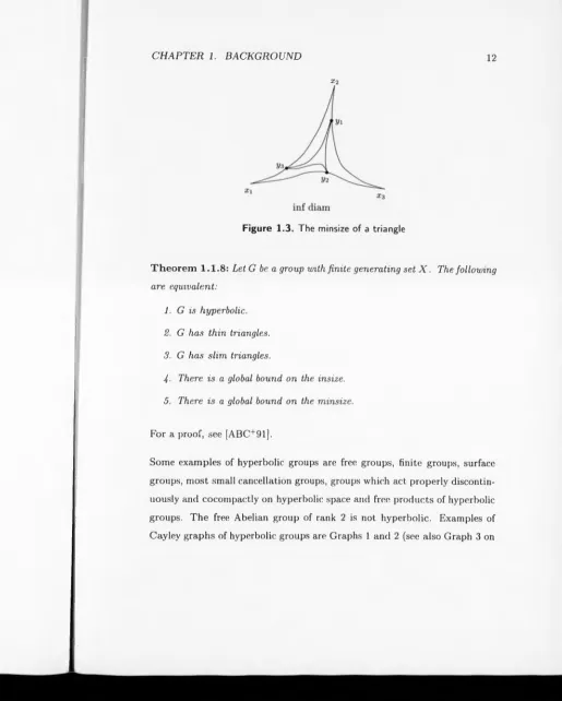
D e fin itio n 1 .1 .7 (M in s ize ): The minsize o f A is (see Figure 1.3)

* 2

Figure 1.3. The minsize of a triangle

T h e o r e m 1 .1 .8 : Let G be a group with finite generating set X . The following

are equivalent:

1. G is hyperbolic.

2. G has thin triangles.

3. G has slim triangles.

4- There is a global bound on the insize.

5. There is a global bound on the minsize.

For a proof, see [ABC+91],

CHAPTER 1. BACKGROUND 13

page 54).

1 .1 .2

T h e B oundary o f a H yp erbolic G ro u p

Hyperbolic groups have a boundary which is a quotient o f the space o f in­ finite geodesics. The boundary is usually described in terms of sequences and the Gromov inner product (1.1). We give here a more geometric ap­ proach using geodesics in the Cayley graph T. The resulting space defines a compactification o f T.

D e fin itio n 1.1.9 (G e o d e s ic ra y ): A geodesic ray, r, is an isometric em­ bedding o f the interval [0,oo) into T (compare with Definition 1.0.2). A

geodesic ray from a: is a geodesic ray r such that r(0 ) = x. A biinfinite

geodesic ray is an isometric embedding of (—00,00) in T.

Let r, s be geodesic rays. We define the equivalence relation, ~ , by r ~ s if there is a constant k such that, for all t, d (r(t), s(t)) SC k,. Suppose that

r and s are geodesic rays from the identity. If T has ¿-thin triangles (see

Definition 1.1.4) and, for some t, d (r (t),s (t)) > S, then, for all u ^ 0,

d (r(t + u), s(t + u)) ^ 2u (see Figure 1.4). So, in this case, if such a constant

k, exists, we can take it to be 6.

CHAPTER 1. BACKGROUND 15

we say that r tends to a, r —> a, r(t) —> a or r(oo) = a. Similarly, if r is a biinfinite geodesic, then we write r ( —oo) = b if the reverse o f r tends to 6.

Let a, b € d r with a ^ b. Then there is a biinfinite geodesic r such that f ( —oo) = a and r(oo) = b. We say that r connects a and b and write r : (—oo, oo) —► (a, b).

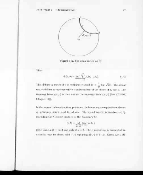
D efin ition 1.1.11 (V isu a l m e tr ic ): We give <?r the visual metric, de(-, •). Fix a base point x0 in T and a constant £ > 0. The first approximation to the visual metric is

I inf exp —(ed (xo,r)) if a ± b,

Pc (a, b) = < r:(-oo,oo)-»(a,6)

I 0 if a = 6,

(1.3)

CHAPTER 1. BACKGROUND 17

a

Figure 1.5. The visual metric on dV

Then

dr( u ,b )= inf y pc(at

chaiiiN £ (1.4)

1

This defines a metric if e is sufficiently small (e < — log(\/2)). The visual 4o

metric defines a topology which is independent o f the choice o f z0 and e. The topology from />,(•,) is the same as the topology from df (•, ■) (See [CDP90, Chapter 11]).

In the sequential construction, points on the boundary are equivalence classes of sequences which tend to infinity. The visual metric is constructed by extending the Gromov product to the boundary by

(a.b) = inf lim (an.6„).

a „ * a n - » o o

bn

with a / b, let r be a biinfinite geodesic ray connecting a and b. Then (a.b) satisfies d (x0,r ) ^ (a.b) ^ d(x0,r ) — 46.

The topology is also independent o f the choice o f finite generating set. So the following definition is consistent:

D e fin itio n 1.1.12 (B o u n d a ry o f G ): The boundary o f G is OG = dP.

Note that OG is compact and Hausdorff.

1.2

Autom atic Groups

The information in this section is given in more detail in [ECH ' 92].

1.2.1

F inite State A u to m a ta

An alphabet is a finite set o f symbols. A word is a string o f symbols o f the alphabet A. We use A' to denote the set o f all words over A (including the empty word). A language is a subset o f A '. If w 6 A ’ and n ^ |w|, the length o f w , then w(n) denotes the word given by the the first n symbols o f

w.

A finite state automaton A is the following data:

1. A finite set o f states, S.

2. An alphabet, A.

CHAPTER 1. BACKGROUND 19

the first coordinate is called the source of e. The projection t onto the second coordinate is called the target e. The projection l onto the third coordinate is called the label o f e.

4. Two subsets I and Y o f S called the initial and accept states.

The automaton A can be drawn as a directed graph with each state being a vertex and each edge being a directed edge from its source to its target.

An edge path is a sequence of edges e j,e2, . . . , e n such that t(ei) = s(ei+1). The edge path e i,e2, . . . , e „ defines the word w = l{e\ )l{e2) ■ • • l(en) in A '.

If s(ei) € / and £(en) 6 Y , then we say that the word w is accepted by A- That is, there is a path in .4, labelled by w, starting at an initial state and ending at an accept state. The language accepted by A is the set o f words accepted by A.

1.2 .2

A u tom atic G roups

Let G be a group with finite generating set X . We assume that X is closed under taking inverses. There is a natural projection from words over X onto

G.

D efin ition 1.2.1 (a u to m a tic g r o u p ): The group G is automatic if there are the following finite state automata:

1. The word acceptor with alphabet X which accepts at least one repre­ sentative for each element of G.

{$ } x X U {$ } which accepts all pairs o f padded words (w\,w2) such that W\ and w2 are both accepted by the word acceptor and such that, in G, w tx - w2.

1.2 .3

H y p erb o lic G ro u p s

Hyperbolic groups are automatic. There are two special automatic structures which are used in this thesis.

Firstly, there is the geodesic automatic structure. The word acceptor accepts the set o f geodesics. For each g 6 G, any shortest representative of g is accepted. We call this word acceptor the geodesic acceptor. The property of having an automatic structure with a word acceptor which accepts the set of all geodesics is called strongly geodesically automatic. A group is strongly geodesically automatic if and only if it is hyperbolic.

Secondly, there is the ShortLex automatic structure. The generators are given an order. For each g € G we take the lexicographically least geodesic; that is, among shortest representatives for g, we take the one which comes first in the lexicographical order. There is an automatic structure whose word acceptor accepts the set o f all ShortLex representatives.

Another important automaton is the word difference machine. T h is automa­ ton accepts pairs of geodesics and keeps track o f the word difference (in the group) at each stage. The word (w t, w2) is accepted if and only if, for every

CHAPTER 1. BACKGROUND 21

automatic structure for a hyperbolic group.

1.3

Computability Problems in Groups

We say that we can determine whether a group has a given property if there is an algorithm (which can be implemented by a Turing machine) which outputs ‘yes’ if the property is true and ‘ no’ if the property is false. Partial algorithms, which output ‘yes’ if the answer is true but may not terminate if the answer is false (or vice-versa), are often much easier to find.

The question of whether a particular problem or property can be solved algorithmically is a difficult one. The most famous negative answer is the unsolvability of the word problem [Nov55, Boo57]. That is, there are groups such that there is no algorithm which takes as input a word in the generators and outputs whether the word equals the identity. A related question is; can one can determine whether a given presentation defines the trivial group? Again the answer is that there is no algorithm which takes as input a finite presentation and outputs whether the group defined by the presentation is trivial. However, given the automatic structure o f a group, one can solve these problems.

use this to compute other properties.

1.3.1

C o m p u ta b ility in H yperbolic groups

We have already seen that hyperbolic groups are a special kind o f automatic group. We ask what properties o f a hyperbolic group we can compute.

Suppose we are given a presentation G = (X | R) for a group which we know to be hyperbolic; then:

1: The word problem is solvable (see the discussion above).

2: The problem o f deciding whether G is trivial is solvable (see the dis­ cussion above).

3: We can solve the conjugacy problem in G. That is, given u ,v € G, we can algorithmically determine whether u is conjugate to v.

4: We can compute the constant o f hyperbolicity, (5 (see [EH], also Theo­ rem 2.1.4).

5: We can list the elements o f finite order up to conjugation. That is, we can write a (finite) list such that for every finite order element g G G, the list contains a conjugate o f g. (We can refine the list so that it contains exactly one conjugate o f each finite order element.)

CHAPTER 1. BACKGROUND 23

power of h also has length ^ 4 (5 + 1 . So for each element o f length ^ 46 + 1

we just need to compute powers and reduce until either we have the identity,

or we have an element o f length greater than 4(5 + 1. □

6: We can list finite subgroups up to conjugation. That is, we can write a (finite) list such that, for every finite subgroup H o f G , the list contains a conjugate o f H .

P r o o f: Each finite subgroup is conjugate to a subgroup o f diameter ^ 10(5+1 ([BG95]). There are a finite number o f such sets. We can systematically write

down all such sets and check whether they form a group. □

7: We can compute the integral homology and cohomology o f G. That is, given n, we can compute Hn(G, Z) and Hn(G ,Z ) (see Chapter 2, Theorem

2

.

.

).

Recall that a group has 0, 1, 2 or infinitely many ends.

8: There is an algorithm to determine whether G has 0 ends and whether

G has 2 ends. There is a partial algorithm to determine whether G has

infinitely many ends.

strong components. A group has 2 ends if and only if the group has ‘linear’ strong components with no path to another linear strong component. Both these conditions are detectable.

To detect if a group has infinitely many ends, make successive approximations to the boundary (see Chapter 3). If there is ever more than 1 component then there must be infinitely many ends (see Proposition 3.3.13). □

R em a rk : Andrew Clow has implemented an algorithm which detects if an automatic group has infinitely many ends (see [Clow]).

Q u estion 1 .3.1: Can we compute the number o f ends o f G'f

R em ark : From the discussion above, we are left with the problem o f finding an algorithm which detects if a group has 1 end.

Q u estion 1.3.2: Can we compute the dimension o f the boundary of G'f An upper bound can be computed (see Proposition 3.3.6).

Q u estion 1.3.3: A theorem o f Delzant’s [Del91] says that a torsion free hyperbolic group has only finitely many conjugacy classes o f non-free, two- generator subgroups. Can we algorithmically list these?

CHAPTER 1. BACKGROUND 25

can we tell whether the subgroup generated by {w b . . . , wn} is free on these generators?

1 .3 .2

Unsolvable P rob lem s in H y p erb o lic G roups

Some problems in hyperbolic groups are known to be unsolvable. The results here are given in [BMS94] using a construction o f Rips [Rip82]. Given an arbitrary finite presentation for a group H , the Rips construction gives a hyperbolic group G ( H) with a natural epimorphism onto H such that the kernel K is generated by 2 elements. That is, the following sequence is exact;

where H has an arbitrary presentation, K can be generated by 2 elements and G is hyperbolic.

U n so lv a b le P r o b le m 1.3.5 (R ip s [R ip 8 2 ]): The generalised word prob­ lem is unsolvable in hyperbolic groups. That is, there is no algorithm which takes as input a finite presentation o f a group G which we know to be a hyperbolic, a subgroup H of G given by a finite set o f elements o f G which generate ii and an arbitrary word w in G and outputs whether w € H .

U n s o lv a b le P r o b le m 1.3.7 (B a u m sla g, M iller, S h ort [B M S 9 4 ]): The rank (minimum number of generators) o f a hyperbolic group is not com­ putable. This follows from the unsolvability of the isomorphism problem for an arbitrary presentation. Let H be the group defined by an arbitrary presentation. Perform the Rips construction on H * H * H. The hyperbolic group G ( H * H * H) has rank 2 if and only if H is trivial, otherwise it has rank at least 3. If we can compute the rank of G, then we can compute whether H is trivial.

U n s o lv a b le P r o b le m 1.3.8 (B a u m sla g, M iller, S h ort [B M S 9 4 ]): There is no algorithm which takes as input a finite presentation o f a hyper­ bolic group G and a subgroup H of G given by a finite set of elements of G which generate it and outputs whether the subgroup H ;

1. is G,

2. has finite index,

3. is finitely presented,

4. has finitely generated second integral homology group,

5. is normal,

6. is a maximal proper normal subgroup,

7. is root-closed,

Chapter 2

Computing the Homology of a

Hyperbolic Group

C h ap ter S u m m a ry

We show that there is a Turing machine which has as input a finite presentation o f a hyperbolic group G and as output the nth inte­ gral homology and cohomology groups Hn(G , Z ) and H n(G, Z ), for any given n. In Section 2.1 we recall the Rips construction of a simplicial complex on which G acts rigidly, with finite stabilis­ ers and with finite quotient. In Section 2.2 we amend the space using the theory o f complexes of groups, introduced by Haefliger in [Hae91], so that the action is free and the quotient is finite in each dimension. The quotient space is computable by a Turing machine and so its homology groups are computable.

2.1

Constructing a Contractible Space with

Rigid G-action, Finite Stabilisers and Fi­

nite Quotient

Let G be a hyperbolic group.

D efin ition 2.1.1 (R ip s C o m p le x ): Fix a generating set for G and fix a constant d. The Rips complex Pd is the simplicial complex with simplices (vo,. . . , vn) for every set {uo,. . . ,v n € G \ V i,j, |wj — Vj\ < d}. The group

G acts on Pd by g(vo , . . . , vn) = (gv0, . . . , gvn). This action is simplicial and

the action on the vertices is free and transitive.

T h e o r e m 2.1.2 (R ip s ): Let G be a 6-hyperbolic group. If d 2? 45 + 1 then the Rips complex Pd is contractible, finite dimensional and the stabiliser of

each simplex is finite. If G is torsion free then the action is free. (See, for

example, [GdlH90, Chapter f ].)

Let P'd denote the first barycentric subdivision of Pd. We say that a group action on a simplicial complex is rigid if whenever a group element stabilises a simplex, it acts as the identity on that simplex. This is a natural generali­ sation o f acting without inversion on a graph.

L em m a 2 .1.3: The action o f G on P['d is rigid.

CHAPTER 2. HOMOLOGY OF A HYPERBOLIC GROUP 29

permute the vertices o f a non-trivially. □

T h e o re m 2.1.4 (E p stein , H o lt [E H ]): //u ;e are given a presentation for

a group G and we know that the group is hyperbolic then we can compute 6.

C o ro lla ry 2 .1.5: We can compute the quotient G\Pd.

P r o o f: Theorem 2.1.4 tells us that we can compute 6. We can then fix d = 45 + 1. Every simplex in G\P(i is the quotient o f a simplex in Pd

containing the identity vertex (because the G-action on the vertices o f P,t is transitive). The ball o f radius d is finite; therefore we can list every simplex in G\Pd and the boundary maps hence all the simplices in G\P'd. □

Note that, in the case when G is torsion free, the homology o f G is the homology o f G\P'd and Corollary 2.1.5 tells us that we can compute this space. The fact that G\P'd is finite enables us to compute the homology of

G.

Lem m a 2.1.6: Given, a simplex o f P'd, we can compute its stabiliser.

P r o o f: By Lemma 2.1.3, if g 6 G stabilises a simplex, it stabilises each vertex. Each vertex o f P'd is a finite subset o f G. Each element o f the stabiliser o f the vertex {ffi,. . . , g „ ) has the form g,gJ ', for some 1 ^ t, j ^ n. We can check which o f these elements stabilise the vertex and hence find the stabiliser o f any vertex. The stabiliser o f the simplex is just the intersection

C o r o lla r y 2.1.7: We can write a list o f stabilisers o f simplices o f P'd which

contains one representative from each G-orbit.

P r o o f: There are finitely many G orbits in Pd so we have finitely many conjugacy classes of stabilisers. We can compute a representative stabiliser

for each conjugacy class. □

2.2

Constructing a Contractible Space with

a Free G-action and Finite Quotient in

Each Dimension

We now assume that we are given a contractible simplicial complex X on which the hyperbolic group G acts rigidly, with finite stabilisers and finite quotient. In Section 2.1 we showed how to construct such a space. We amend this space so that the action becomes free while the space remains contractible. The amended space is no longer finite but it remains finite in each dimension. Our main tool will be complexes o f groups which were introduced by Corson [Cor92] and Haefliger [Hae91].

Let X — G \ X . For every simplex a C X choose a simplex a C X lying above

CHAPTER 2. HOMOLOGY OF A HYPERBOLIC GROUP 31

classifying space o f the category G „ defined by Segal in [Seg68, Section 3] and repeated below. The information for gluing in the E (G „, l ) ’s is obtained from the simplicial cell complex o f groups description for G given by its action on X .

For a group G, the category G is defined as follows: The set o f objects is G. There is a unique morphism between any pair o f objects; for every g ,h € G, we have the morphism, g~'h, from g to h. The morphisms correspond to multiplication in the group and are composed in the obvious way. This cate­ gory is equivalent to the trivial category with one ob ject and one morphism, therefore its classifying space is contractible (see Section 2.2.4).

2 .2 .1

Sim plicial Cell C om p lexes o f G ro u p s

A simplicial cell complex o f groups is a simplicial cell complex Y with a group associated to each simplex. We use G „ to denote the group associated to the simplex a. Let r be a simplex o f Y and let a be a simplex in the closure o f r (so that a is a simplex o f lower dimension than r which is incident to r). Then there is an injection from C T to G „. We take the barycentric subdivision Y ‘ o f our simplicial cell complex Y so that we have a group at every vertex and an injection, ipa, for every directed edge, a. We require that the following conditions hold:

on page 33),

6

t --- ► a

P

there is an element ga,b £ G p such that the following diagram commutes up to conjugation by gay,

That is, Conj(0o,fc) o ipab = ipa o ipb (where Conj(/y): x gxg~ x).

2. For every triple o f connected edges a ,b ,c (a tetrahedron in Y'), T

the ‘conjugators’ satisfy ipa(tlb,r)ga,bc = 9a,b9ab,c-

See [Hae91] for a more detailed exposition.

CHAPTER 2. HOMOLOGY OF A HYPERBOLIC GROUP 3 3

P

O p ,a CT

(a) X ' (b) X

Figure 2.1. The conjugator ga<b = g„'ag~'rgp,T

2 .2 .2

R eturning to our Situation

In the barycentric subdivision X ' o f X , with edges directed towards the vertices o f X , we have a group G„ at each vertex a. For each directed edge b in X ' (joining r to a ), choose g „ r € G such that g „iT (n) C T in X (see Figure 2.1). Note that g „ T is unique up to left multiplication by an element o f G T. We define the injection ipb : Gr —> G„ by ipb(h) = ga \hgaT. (Changing g„tT is the same as composing ip with an inner automorphism of

G r.) For every pair of composable edges a, b in X ' (a triangle b,a,ab in X '

corresponding to a triple o f simplices r, a, p in X with r D a D p, see Figure 2.1(a)), we define the conjugator gnb = gp '„g„'Tgp,T (««• Figure 2.1(b)).

L e m m a 2.2.1 (HaeHiger [H ae91]): Tlic above description defines a sim-

plicial cell complex o f groups presentation fo r G. □

2 .2 .3

T h e Fundam ental G ro u p o f a C o m p le x o f G ro u p s

We have a group Ga for each vertex er o f X ' and an injection for each directed edge. We use s(a) and t(a ) to denote the source and target vertices o f the directed edge a. We associate to each edge, a, the element ga = gt{a),,(a) € G, so that ga(t(a)) is incident to s(a). Occasionally we want to use a to denote not moving, in which case s(a ) = t(a) and ga = 1. Note that, by construction, the elements ga satisfy the relations gab = gbgaga,b and that ipa (g) = ga 1 gga.

A G-path in X ' is a path in X ' with additional information to define an element of G. It is defined as follows: Trace a path in X'. Every time we traverse an edge, a, we multiply on the right by ga. When we reach a vertex (including the initial vertex), a, we multiply on the right by an element of

G „. This path can be written as a sequence go(io9iOi92 ■ • -an- i gn, where a,

is an edge, .<>(«,f ] ) = t(cij), g} € G ,(n>) and g,t G G t(a„)- The set o f closed G-paths can be multiplied in the obvious way to form a group. This group is the fundamental group o f the complex of groups and it is isomorphic to G.

2 .2 .4

C ategories and Classifying Spaces

We reconstruct the space X ' using the language o f category theory. We give two naturally isomorphic categories whose classifying spaces are respectively

X ' and a space with a free G'-action. A result o f Segal’s (Proposition 2.2.2)

tells us that they are homotopic; hence we have our desired space.

CHAPTER 2. HOMOLOGY OF A HYPERBOLIC GROUP 3 5

set of morphisms, 2-simplices the set o f commutative triangles, and so on (see [Seg68, Section 2]). A group action on a category extends to an action on the classifying space.

Two categories are equivalent if there are functors between them such that each composition, T , is a natural isomorphism from the category to itself. That is, there is a natural transformation (morphism o f functors) between the identity functor and T such that each induced morphism is invertible. In other words; for every object, Ob, and for every morphism, / from Ob to Ob', there are invertible morphisms, v and i /, such that the following diagram commutes:

Ob — v—+ T(O b)

I'

I”

Ob' —^ T {Ob').

(See [Mac71, Page 16]).

P r o p o s it io n 2.2.2 (S e g a l): The classifying spaces of two equivalent cate­

gories are homotopic ([Seg68, Proposition 2.1]).

D e fin itio n 2.2.3 ( C C ) : Our first category has objects (gG a,cr) where a is a simplex in X and gG „ is a coset of the stabiliser group G „. The nontrivial morphisms from (g G „ ,a ) are labelled by edges a with s(a) = a\

{gG,(a), s(a)) y (ggaG t(a),t{a)).

L em m a 2.2.4: The classifying space B C C o f C C is X '.

Proof: Let C (X ) be the category associated to X . Its objects are the

simplices o f X and its non-trivial morphisms are the directed edges o f X ' . The classifying space o f C (X ) is X '.

Define the map F : (gGa, o ) go from the objects of C C to the objects

o f C (X ) . Recall that ga is such that ga(t(a)) is incident to s(a), so there is an edge g(a) in X ' connecting s(a) and ga(t(a )). Consequently, for each morphism a, we have the following commutative diagram:

(gG i(tt),s (a ) ) ---y (ggaG t(a), t(a))

F

g { s ( a ) ) --- —— * {gga(t(a ))).

So the map F extends to a functor.

The inverse map F ~ l : go (gGa,o ) is also a functor. Hence F and F ~ l

are natural isomorphisms of categories. Lemma 2.2.4 follows from Proposi­

tion 2.2.2 and from the fact that F is a bijection. □

D e fin itio n 2.2.5 ( G C ): The objects o f our second category, which we call G C (G (X )) or G C (‘group category of G ( X ) ’ ), are pairs (g ,o ) € G x Simplices o f X . The morphisms are

(g,s(a )) - ^ 4 (gka,t (a )),

where ka(t(a )) C s(a) and a is either a directed edge in X ', or s(a) = <(a). Note that, ka = g„gt(a) for some gt^ 6 so the morphisms can be thought

CHAPTER 2. HOMOLOGY OF A HYPERBOLIC GROUP 3 7

o f as (traverse an edge then) multiply by an element o f the stabiliser group G ((a). The morphisms are composed in the obvious way; (a ,k a) o (b,kb) = (ab,kakb) whenever it is defined (when s(a) = t(b)). Observe that, since

t(ab) = t(b), s(ab) = s(a) and t(a) = s(b), we have

kakb(t(ab)) C ka(t(a)) C s(ab).

If s(a) = t(a) we sometimes write the morphism as k, where k € G s(„). These are the only invertible morphisms in G C . There is a G-action on the objects o f G C given by g(g',cr) = (gg',o). Clearly, this action is free.

P r o p o s itio n 2.2.6: The action o f G on the classifying space B G C is free.

P r o o f: Each simplex o f B G C comes from an ordered set o f objects of GC. So if g fixes a simplex, it must fix each of the objects (permuting them will

change the order). But the action on the objects is free. □

We will now define the functors P : G C —> GG (projection) and R : C C —► G C (inclusion given by a choice o f coset representatives, {h gc „ } , one repre­ sentative for every coset of each stabiliser group).

D efin ition 2.2.7 ( P ) : The projection functor, P : G C —> G G , is defined by

P : (g, a) •-> (gG „, o ) on the objects and by P : (a, ka) H a o n the morphisms.

the following diagram commutes;

-> (gka, t(a))

G C (g ,s(a ))

C C (gGs(a)i ®(®)) t (gkaGt(a),i(a)).

Note that, since ka = gagt(a) for some gt{a) e G ((a), gkaG t(a) = ggaG

t(a)-D efin ition 2.2.8 ( R ) : Choose a set o f coset representatives { } , one for each coset o f each stabiliser group. If we write h\ = hgo Mat and h2 = hggao l(a),

then hi = ggs(a), h2 = gka for some gs^ € G ,(a), and for some ka such that ka(t(a)) C s(a). So h\lh2 = </7(a)^“ and

h i'h2(t(a )) = g;{'a)ka(t(a)) C g^a)s(a) = s(a).

We define R : C C —> G C by /i : (gG „, a) ►-» (hga„,cr) on the objects and by R : a >-> ( a , o n the inorphisms. /? is a functor because, for any morphism (gG s(a), s(a )) —^4 (ggaGt(a), t(a)) in GG, the following diagram commutes;

C C (gGs(a), 8(a)) — —> (ggaGt(a), t(a))

R

R R R

, w 'h2) ;

L em m a 2 .2.9: Thu categories C C and G C are equivalent.

CHAPTER 2. HOMOLOGY OF A HYPERBOLIC GROUP 3 9

For the other composition functor R P = R o P : G C —> G C , (g,cr) >

(hgG„ ,o ) , for every morphism, we have the following commutative diagram;

where x = g 'hgGi(a), which is in G S(a) because g and hgG,(a) are in the same coset o f G s(0), and similarly z = (gka)~ l hgkaGt(a) € G t(a)- We need to check that y = satisfies y{t(a)) C s(a). Now, hgG.(a) = yys(a) for some gs{a) e G j(o) and hgkaG,ia) = gkagt(a) for some gtM e G t(a). So y (i(a )) = g ^ k e g tw itia )) C s(a).

Clearly, both x and z are invertible, so R P and Id are equivalent. □

T h e o r e m 2.2.10 : The classifying space B G C o f G C is contractible.

P r o o f: By Lemma 2.2.9, the categories G C and GG are equivalent. By Proposition 2.2.2, the classifying spaces B G C and B C C are homotopic. Thus

B G C ~ B C C = X ' (by Lemma 2.2.4) which is contractible by Rips’ Theo­

rem (Theorem 2.1.2). Therefore B G C is contractible. □

P r o p o s itio n 2 .2.11: For each n, we can list the simplices o f the n-sheleton

o f the quotient space G\BGC.

G C (g ,s(a )) ■» (gka,t(a ))

RP x R P R P z R P

P r o o f: An n-simplex comes from a sequence o f n composable edges. We can

T h e o r e m 2.2.12 :

Given an integer n and a finite presentation for a group G which we know to

be hyperbolic, we can compute the nth (co)homology group o fG .

P r o o f: The nth (co)homology group o f G is the nth (co)homology group of

G\BGC, which is computable and finite in every dimension. Therefore we

can explicitly write lists of the n +1, n and n — 1 cells and the boundary maps (G \flG 'C )("+1> - A (G \ B G C )W (G \ B G C yn~ll The problem reduces

to the problem o f finding the kernel and image o f linear maps in free-Abelian

groups, which is computable. □

The category C G ( X ) in [Hae91] and [Hae92] is precisely G\GC. Haefliger shows in [Hae92] that this category is naturally isomorphic to the category

G x C (X ) (which we describe below) and that the classifying space of this

category is homotopy equivalent to B G x0 X = G\BG x X , where B G is an

E(G , 1) and G has the diagonal action on B G x X . BG x c X is sometimes

called the Borel construction or Bond homotopy quotient (see, for example, [Geo]). The category G tx C ( X ) has objects the cells d o f X and, for every

(/ 6 G and for every ff, it has a morphism d % yd. When X is contractible,

BG xq X is a K (G , 1). See Figure 2.2 for a map o f the different proofs.

2.3

Examples

E xa m p le 2 .3.1: An easy first example is Z :t = (x | x 3). The Rips complex

CHAPTER 2. HOMOLOGY OF A HYPERBOLIC GROUP 41

C (X ) =* C C “ G C

B C (G (X ))~ B (G x C ( X ) ) ~ B G x G X

Figure 2.2. A diagram showing the relationships between the different cate­ gories in this chapter and in [Hae92], The down arrows marked B are geometric realisations.

about the barycentre of the 2-simplex. The stabiliser of the 2-simplex is Z 3, all other stabilisers are trivial. Taking the barycentric subdivision makes the action rigid with one vertex stabiliser group Z3 and all other stabilisers trivial (see Figure 2.3).

We choose representatives for each Z 3-orbit in P{ as shown in Figure 2.4. The stabiliser o f u3 is Z 3, all other stabilisers are trivial.

Figure 2.3. The Rips complex of Z3 = (x \ x 3) and the stabilisers of the simplices.

Figure 2.4. Choosing representatives in each orbit

CHAPTER 2. HOMOLOGY OF A HYPERBOLIC GROUP 4 3

Figure 2.6. Part of the tiling by (7r/2, 7t/3, 7r/7)-triangles. The shaded area is a fundamental domain for the action of (2,3,7)-triangle group on this tiling.

E xa m p le 2 .3.2: A better example is the orientation preserving (2,3,7)- triangle group ( x ,y ,z \ x 7, y 3, z2, zyx). We proceed from Section 2.2 using a

tiling o f the hyperbolic plane by (7r /2, 7t/3, 7t /7)-triangles as our contractible space on which the group acts rigidly and with finite stabilisers. Call this simplicial complex X . The action is generated by clockwise rotations through

7t/7, 7t/2 and n/3 about iq, C2 and ^3 (the vertices in the shaded region o f Figure 2.6) respectively.

A fundamental region for our action is a quadrilateral (for example, the shaded region in Figure 2.6). The quotient space is homeomorphic to a sphere (Figure 2.7).

Figure 2.7. The quotient space for the (7r/2, 7t/3, 7r/7)-triangle tiling under the action of the (2,3,7)-triangle group

For a pair o f incident simplices a, r in X , we need to choose a g„iT € G such that g„tT(a) is incident to t. In most cases we can choose the identity. The

only exceptions being between the pairs (cr2, e j), (a2,u2) and (<72,e 3) (see Figures 2.7 and 2.6). We take g„2<V2 - ga2,c3 = x and g„2,e, = y~ l and label

edges in the barycentric subdivision o f X accordingly (see Figure 2.8(a)). The triangle in X ' with vertices at,ej,Vk has conjugator gai,ej9ej ,vt9a%\Vk and

so most are trivial. The exceptions are shown in Figure 2.8(b).

Wo now construct the category GC. Recall that the objects are labelled by pairs (g, a ), where g € G and a is a vertex in X ' . The morphisms come from traversing an edge in X ' (or staying put) followed by multiplying by an element o f the stabiliser group o f the destination vertex.

We can label each simplex lying above a in the original complex by a coset of

CHAPTER 2. HOMOLOGY OF A HYPERBOLIC GROUP 4 5

Figure 2 .8 . Labelling edges and finding conjugators. Unmarked edges in the left picture and unmarked faces in the right picture are labelled by e.

Figure 2.10. The quotient space G\BGC for the (2, 3, 7)-triangle group.

representative and g„ 6 G„. The faces of our tiling X have been labelled in Figure 2.9.

The 1-skeleton o f the quotient space G\BGC is shown in Figure 2.10. The space G\BGC looks spherical, but the 2-cells don’t ‘ match up’ so there aren’t any embedded spheres. The third homology group is Z. The 2-cells have to be ‘wrapped around’ 42 times until they match up. This coincides with the second homology group being Z « - The first homology group, the abelianisation o f G, is trivial.

CHAPTER 2. HOMOLOGY OF A HYPERBOLIC GROUP 47

Chapter 3

The Boundary of a Hyperbolic

Group as an Inverse Limit of

Finite Sets

C h a p te r S u m m a ry

Given a hyperbolic group G, we show how to construct an inverse system o f finite topological spaces whose inverse limit is homeo- morphic to dG, the boundary o f G. Each o f the finite spaces are computable and can be used to estimate topological properties o f the boundary.

Let G be a hyperbolic group and fix a generating set. Let T be the corre­ sponding Cayley graph. Recall (Section 1.2.3) that G has a ShortLex auto­ matic structure and a geodesic automatic structure.

3.1

The Boundary as an Inverse Limit

3.1 .1

C on stru ctin g Finite Topological Spaces

Let Wn denote the set of elements o f length n in G. The set Wn can be thought o f as the set o f ShortLex geodesics of length n in I\

D efin ition 3.1.1 (clu s te r): A set o f ShortLex geodesic rays (geodesic rays such that every prefix is a ShortLex geodesic) to the same boundary point is called a cluster o f geodesic rays or a cluster.

D efin ition 3.1.2 (fr o n d ): The set of truncations o f length n of the geodesics in a cluster is called the nth frond o f the cluster. A frond o f length

n or, frond , is a subset of Wn such that each element o f the subset can be

extended ShortLex geodesically to the same boundary point. We call a frond with k + 1 points a k-frond. Note that elements which cannot be extended ShortLex geodesically to the boundary are not fronds.

CHAPTER 3. THE BOUNDARY AS AN INVERSE LIMIT 51

M { * , » } { y )

F

” ( { * } ) « ({? /})

s

Figure 3.1. The relationship between F, W and S

o f length n by truncating each element o f the cluster at length n. Thus we have a map p „: {clusters} —> Fn.

3 .1 .2

T h e Restriction M a p

We define the map pn : Wn —¥ W n-1 by

Pn

1

l,

where each a, is in the generating set and a\ ■ ■ ■ an traces a ShortLex geodesic in T. The map p restricts a geodesic of length n to itself truncated at length

n — 1.

D e fin itio n 3.1.4 (T h e r e s tr ic tio n m a p ): The map pn extends to a map

from Fn to by

fn- Fn ->• F„_ i , {w 0, w i , {p (w 0), p{wx) , .

..,

.

The map / „ is called the restriction map. The image o f a frond is clearly a frond. A /c-frond maps to a j-fron d, for some j ^ k. Recall the map pn from Definition 3.1.3. The restriction map satisfies pn ° fn = P n -1! that is, for each n, the following diagram commutes:

Now, if x ,y G Fn and x G y, then f„ (x ) G f n(y)- Since S„ exhibits the topology o f Fn, we can think of / „ as a map from Sn to Sn- i .

{clusters} > Fn

(3.1)

CHAPTER 3. THE BOUNDARY AS A N INVERSE LIMIT 53

Figure 3.2. F t , part of the Cayley graph and S\ of the fundamental group of a surface of genus 2

The fronds o f length 1 are the generators and pairs { x ,y } such that y~ lx appears in the relator written cyclically (see Figure 3.2).

Part o f the restriction rnap f2 is shown, as a map S2 —► S\, in Figure 3.3.

3 .1 .3

T h e Inverse Lim it

The finite sets Fn and the maps / „ : F„ —> Fn | form an inverse system, which we call F:

(3.2)

We now look at the inverse limit o f F, F.

CHAPTER 3. THE BOUNDARY AS AN INVERSE LIMIT 55

Figure 3.3. The restriction map f2

1, f i(x i) = x i -1- Since, for each i, fio p i = p,_i (3.1), a cluster corresponding to j is a cluster corresponding to x l. So we can extend the maps pn to a map p: {clusters} —► {imF. The map p is a bijection, so a point in lim F can be thought o f as a cluster (that is, a set o f geodesic rays to the same boundary point). The closure of a point x = (a:*)“ , in {im F is given by

x = { y = (y<)“ i |Vi, yi e x ; } .

Equivalently, y € x if and only if p~*(y) C p~ *(x).

D efin ition 3.1.6 (T h e m ap k ): The point x in (im F naturally defines the cluster p~l (x), which is a set of geodesic rays to the same boundary point £. We define the map k : {im F —y dG by k (x) = £. Every infinite ShortLex geodesic is a cluster, so the map k is a surjection.

P r o o f: There are only a finite number o f ShortLex geodesic rays to each boundary point, so there are a finite number o f clusters to each boundary

point. □

In fact, there is a universal bound on the size o f '(0 1 (see Lemma 3.3.2 on page 68).

3 .1 .4

H ausdorffifying the Inverse Limit

The space hm F is not necessarily Hausdorff because the closure o f a point is not necessarily itself.

To make Urn F Hausdorff, we amalgamate certain points. We amalgamate the points x and y if there is a z € Urn F such that x € z and y € z. If x and

y define the same boundary point, then p 1 (x) and p 1 (y) are clusters to the same boundary point. Therefore p 1 (x) U p 1 (y) is a cluster, so we can set

z = p\p '(x ) U p '(?/)]. Then x and y are both in z. So we amalgamate x

and y if and ordy if they define the same boundary point. Equivalently, we amalgamate x and y if and only if k(x) = k.(y). Lemma 3.3.2 shows that this process is finite at each point.

Let II denote the space we obtain by performing the above operations and let y : Urn F —> / / be the quotient map.

L em m a 3 .1.8: The pan //,</ has the property that for all Hausdorff spaces,

CHAPTER 3. THE BOUNDARY AS AN INVERSE LIMIT 5 7

l, such that the following diagram commutes:

(im F — ^ H

Y.

P r o o f: Let Y be a Hausdorff space and let c be a continuous map from (im F to Y. Let x, y €. JimF such that q(x) = q(y). Then there is a z in (im F such that x ,y € z. Then c(x) = c(z) = c(y) because c is continuous and

x € z ==> c(x) e c(z ) = (c (z )}. So the map l must be 1(a) = cq~1(a).

(Although q~l is not a map, cq~l is a map.) The map c is continuous and q

is a quotient map, so l is continuous. □

In particular, in the case when Y = dG, we have the following commutative diagram;

We shall show that the map k is continuous and deduce that h is a homeo- morphism (Theorem 3.1.15).

3 .1 .5

T h e T opology o f H

It is useful to first examine the topology o f (ini F. Let x n € Fn. The set

(im F H

(3.3)

is called a cylinder (compare with Definition 4.1.2). Note that fixing the nth entry o f a sequence in ^im F fixes all earlier entries. So a cylinder is fixed on a finite number o f symbols but can then vary arbitrarily. We also refer to finite unions o f cylinders sis cylinders. The complement o f a cylinder is itself a cylinder.

Recall that a basic open set in Fn corresponds to the star o f a simplex in Sn; open sets are unions o f simplices in S„ which are open in the CW-topology. That is, given a frond x 6 Fn, there is a basic open set Bx in Fn given by

Bx = (Jjox?/- ^ U is an open subset o f Fn, then fn+l (U) is open in Fn+1,

because, given a frond x € Fn+i , y D x if and only if f n+i(y) D / „ + i(x ). So the inverse image o f a star is a union o f stars. So, if U is open in Fn, then its inverse image in Fn+m must always be open.

So a basic open set in ^m F is a set o f the form

C (B X) = ( J C (y )

y e B x

where x € Fn, for some n; that is, a basic open set in (im F is the cylinder o f a basic open set in Fn. An open set in |im F can be written as a union of cylinders o f stars.

L em m a 3 .1 .9 : Any closed set o f Lim F can be made by taking (finite unions

and) arbitrary intersections o f cylinder sets.

P r o o f: Let £ be a closed set. Then E — U' for some open U, where U' denotes the complement o f U. Now, U = (J C\, where C\ are cylinder sets.

CHAPTER 3. THE BOUNDARY AS AN INVERSE LIMIT 5 9

= ( u c > ) ' - n « A € A

But C'x is a cylinder and the result follows.

□

Note that the converse is not true; if you take an arbitrary intersection of (finite unions of) cylinders, then you do not necessarily get a closed set.

Observation 3 .1 .1 0 : An open set U is characterised by the property that if

C (x ) C U (where x € Fn) and x C y then C (y) C U .

Observation 3 .1 .1 1 : A closed set, E , is characterised by the property that

if C (x ) C E and x D y then C (y ) C E.

Now, a closed set in H is a set, E, such that q~l (E ) is closed in (irri F. Similarly, an open set, U, in H is a set such that q ~ '(U ) is open in ljin F.

We now examine the topology o f OG.

Definition 3.1.12 (Shadow): Let g G G. The shadow o f g, which we denote by S(g), is the subset o f OG defined by the set o f geodesic rays from the identity through g. Let uj = {w\, . . . ,u>*} G Fn, then the shadow of ui is

S (u ) = f l, S(w,).

Lemma 3.1.13: Shadows are closed. That is, f o r each g € G, S(g) is

closed.

Fig ure 3.4. A geodesic quadrilateral

geodesic r, from e to through g. By passing to subsequences, for each

n > |<?|, we can ensure that the r, agree on the first n symbols. This gives us

a geodesic ray r from e to lim£j through g. So lim£j € S (g ). □

Lemma 3.1.14: IfU C dG is open and r is a geodesic ray from the identity

such that r(oo) G U, then there is an n such that S (r(n )) C U. Further, if

B = B (r(n ),S ) denotes the ball o f radius 6 about r(n) then (J S(g) C U. geB

Proof: Let r\ = r(oo) and let £ G U S(g). Then there is a geodesic ray

9€B(r(n))

s from e to £ which passes within <5 o f r(n ). So there is an m ^ n—6 such that

d (s (m ),r(n )) < <5. Consider the quadrilateral with edges [r(n),r]) = f||ni00),