Clustering Analysis of Collaborative Tagging Systems
By Using The Graph Model
Jong Youl Choi
Dept of Computer Science
Indiana University at Bloomington
([email protected])
Abstract
We propose a newgraph model for folksonomy analysis. In order to compare our proposed model with the vector space model, which is widely used in the information retrieval field, we have performed multidimensional scaling schemes and clustering analysis by using the both models. While the vector space model is easy to implement in folksonomy analysis and even computationally lighter, the graph model is more suitable for analyzing folksonomies which can be represented as a tag graph. To overcome computational burdens occurred in the graph model, we implemented a parallel version of Floyd-Warshall algorithm for finding the shortest paths.
1
Introduction
As the number of virtual on-line communities has been rapidly growing for a recent period in the Internet, the quantity of information and knowledge produced by the on-line community are measureless. The interesting aspect of this trend is that the knowledges in the Internet are not only produced by a small number of experts, but also they are produced by the normal Internet users. Ratings, recommendations, and collaborative tags are one of those examples. The termfolksonomies, meaning the knowledges collected from the people, has been coined to describe such phenomena. However, such knowledges often suffer from lack of efficiency in searching and discovering meaningful information. This is simply because i) the amount of data to process for searching purpose is huge, ii) the data is not well organized since no single authority can exist, and iii) there is no uniform semantics agreed by all Internet users. As a result, knowledges are often hard to search or quickly buried in by other newly created knowledges as time goes. Many efforts has been taken and lots of researchers have been conducted to solve this problem.
t1 t2 t3
A=
d1
d2
d3
d4
w11 w12 w13
w21 w22 w23
w31 w32 w33
w41 w42 w43
[image:2.612.176.447.72.179.2](a) (b)
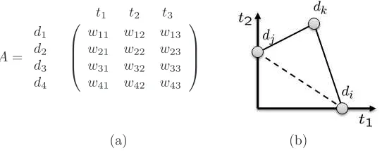
Figure 1: An example of document matrixA using the vector space model of 3-dimension (a) and another example represented in 2-dimension (b). The solid lines in (b) depicts sharing of common tags between two documents and imply their relationships. Note that there is no tags shared between di and dj (depicted as
a dotted line). However they are indeed connected viadk; I.e, they are sharing some information.
by using a query. Through this way, the system can help users to discover unexposed information. Thus, developing precise and efficient models for searching is the key step for building a successful collaborative tagging system.
For building efficient indexing schemes of searching engines, two models have been widely used in the field: the vector space model andthe graph model. Although both models are sharing many similar aspects, they are distinct in many practical point of views. As examples, the Latent Semantic Indexing (LSI) [3] is using the vector space model for indexing and measuring pairwise similarities between documents, and the famous ranking algorithm PageRank used by Google is based on the graph model. While the vector space model has been widely studied and applied in many areas due to its simplicity, not many researches have been conducted for the use of the graph model so far. While the vector space model is easy to apply, the graph model requires additional computational cost – we will discuss shortly – but has more attractive advantages in applying to collaborative tagging systems. Thus, the motivation of this paper is to research on the use of the graph model in performing the analysis of folksonomy data. For this purpose, we will investigate how the graph model is superior to the vector space model in performing clustering analysis. Secondly, how the graph model will behave in dealing with the high volume of data. Finally, we will further research on how to relax complexity of the graph model in order to improve the quality of clustering analysis.
In the next section, we will compare both the graph model and the vector space model and introduce the measurement schemes we used in our experiments. The experiment results are shown in Section 3.
2
Folksonomies Analysis
In the following, we will discuss two models used in folksonomy analysis and introduce measurement schemes we used for experiments.
2.1
The vector space model vs. the graph model
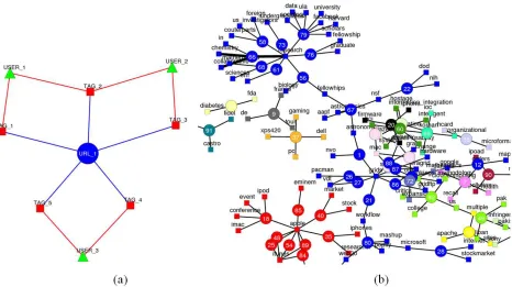
Figure 2: A tag graph(a) and a part of tag graphs of MIS-CIEC portal(b). Tags, resources (URLs), and users are represented as a square, a circle, and a box respectively. (b) shows only resource-tag graphs and each independent network (connected graph) is assigned to a unique color.
whereqequals the total number of distinct tags in the system, and each coordinate stands for one tag word. By using a vector notation, we can represent a documentdi as a q-dimension vector (wi1,· · ·, wiq), where
wij is a weight of the occurrence of the term tj (Various weight schemes are used in the field and will be
discussed shortly) and the collection of n documents as a matrix A ∈ ℜn×q where each row corresponds
to di. An example is shown in Figure 1. Although the vector space model can be immediately applicable
to indexing documents in collaborative tagging systems, it lacks ability to estimate fine-tuned document-document (or tag-tag) relationships. For an example, although two document-documents (or two tags) seem to have no direct relationship by means of sharing no common tags, they may be indirectly connected and share something via other documents. As observed in social networks, such indirect connections can play an important role in searching. As shown in Figure 1(b), the solid lines depict the sharing of common tags between two documents and imply direct relationships of two nodes. Note that there is no sharing tags between di and dj (depicted as a dotted line). However they are indeed connected via dk; I.e, di and dj
are sharing some information. We can exploit this observation for building more efficient searching schemes. However, discovering such relationships is not directly available in the vector space model.
Measurement Abbr Name Definition
Weight
TFtfij Term Frequency The number of tagged termtj for documentdi
DF dfj Document Frequency The number of documents having the same tagtj
TF-IDFtf idfij TF-Inverse DF tfij×logdfnj where nis the total number ofdi
Dissimilarity
COS(di,dj) Cosine 1−Pkwikwjk/
q P
kw2ik
P
kwjk2
JAC(di,dj) Jaccard 1−Pkwikwjk/
P
kw2ik+
P
kw2jk−
P
kwikwjk
PEA(di,dj) Pearson 1−
(P
kwikwjk−1 q
P
kwikPkwjk)
q
(P
kw2ik−1q(
P
kwik)2)(Pkw2jk−q1(
P
kwjk)2)
Table 1: Equations used for measure weights and dissimilarities. Slightly modified from original equations.
edge. Tag graphs in the real life examples tend to be a complex network, showing small world and scale-free network properties [6]. An example of a tag graph is shown in Figure 2(b).
In fact, two models – the vector space model and the graph-based model – can be easily convertible to each other in general. However, they are distinct to each other in various scenarios. Basically, while the vector space model uses vectors in an orthogonal tag basis space, the graph model exploits graphical structures. While the vector space model considers the frequencies of tag occurrences for indexing, the graph model focuses on graphical characteristics such as hop distances and the degree of connectivity between nodes.
2.2
Dissimilarity Measurement
Measuring dissimilarities (or similarities) between two objects is a key step in folksonomy analysis and it is directly related to the performance of the system. Although it is possible in folksonomy analysis to measure various dissimilarities – such as document-document, document-tag, document-user, user-tag, and user-user, in this paper we only consider document-document dissimilarity for simplicity. The other measurements can be easily estimated by using the same technique. Also, we use only dissimilarities to avoid confusion.
Weight Measures:Measuring dissimilarities begins with measuring weightswijfor tagtjand document
diin document-tag matrixA. Various schemes have been suggested in many literatures but the most popular
schemes are Term Frequency (TF thereafter for short) and Term Frequency-Inverse Document Frequency (TF-IDF for short) which is the multiplication of TF and IDF. In a nutshell, term frequency tfij is the
number of tagged term tj for document di and the document frequencydfj is the number of documents
having the same tagtj. IDF is computed by logdfn
j for the total number of document nand thus TF-IDF equalstfij×logdfn
j. Formulas used in this paper are summarized in Table 1.
Dissimilarity Measures: Dissimilarity is a degree of unlikeness between two documents. We used in this paper three common similarity measuring schemes [2]: Cosine, Jaccard, and Pearson. Dissimilarities are simply computed from them. Three dissimilarities used in this paper are defined asCOS,JAC, andPEA,
which summarized in Table 1.
Note that measuring dissimilarity is slightly different in both models. In vector space mode, all document-document dissimilarities can be directly computed from the document-document-tag matrixA; I.e, in the vector space model, we can compute a pairwise dissimilarity matrix D ∈ ℜn×n by measuring its entries δ
ij, meaning
the dissimilarity between two documents di and dj. δij can be computed by using one of our dissimilarity
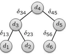
Figure 3: Dissimilarity measure in the graph model. The dissimilarity betweend2and d6 can be computed
by following the connected path. One way to compute this is to find the shortest path fromd2 andd6.
all dissimilarities directly from the matrix A but, instead, we should do iteratively; Firstly, compute only dissimilarities of directly connected documents, i.e., documents sharing at least one common tag between them, and then, measure dissimilarities of the others, which have no direct connections, by means of discov-ering paths between them. Path discoveries can be done by using the solution of the shortest path problem. For an example, as shown in Figure 3, the dissimilarity δ26 cannot be computed at first hand. The value
can be computed after discovering a path fromd2 to d6 or vise versa. When computing dissimilarities by
using the graph model, we don’t always need to find the shortest path. However, in this paper, we choose to use the shortest path for measuring dissimilarities. Floyd-Warshall algorithm [4] is well known for finding the shortest paths. In summary, we can compute dissimilaritiesδij in the graph model by using two steps:
i) measure dissimilarities, likeCOS,JAC, PEA, if documents are sharing common tags, and ii) measure the
shortest path distances as dissimilarities, if ones share no common tags.
In fact, measuring dissimilarities by using graphical structures has been used in the Isomap [9]. In contrast to the Isomap, in which graphical structures should be artificially generated, we utilize the naturally existing graph structures in tag graphs.
Regarding the computational cost, while the vector space model requiresO(n2) computation for obtaining
n×n pairwise dissimilarity matrix D, the graph model using the Floyd-Warshall algorithm needs O(n3).
Considering the number of documents usually maintained in a real system can exceed tens of thousands or even more, the difference of computational cost between the two models will be much larger as the number of documents is increasing. In this paper, we could overcome this problem by implementing a parallel version of Floyd-Warshall algorithms [7] running on multiple processes simultaneously.
2.3
Multidimensional Scaling and Clustering
scaling schemes like Laplacian. Those will be discussed in the experiment result section.
Clustering of folksonomies is an unsupervised way of classification of folksonomy data into several sub groups so that each sub group shares more common concepts while different groups less relateness. In many cases, quality of clustering is measured by the inter-similarity between clusters and/or the intra-similarity within the nodes in a cluster. Euclidean distance is commonly used for measuring inter and intra similarities in the vector space model. However, the graph model can suggest another way of measuring the quality of folksonomy clustering. Since the connections can be obtained from the folksonomy data and those connections can be represented as edges, intuitively we can estimate a clustering result by the number of inter-cluster edges and/or intra-cluster edges; I.e., a good clustering algorithm should produce clusters which maximize the number of inner-cluster edges and minimize the intra-cluster edges. Simply, in this paper, we have devised the following quality functionQto compare clustering results:
Q=
m
X
c=1
Qc= m
X
c=1
P
i,jf(c, eij)
|E| , (1)
where the function f(c, eij) returns 1 if an edge eij between two document di and dj is an inner-cluster
one and otherwise 0 for a given number of clusters c and |E| is the total number of existing edges. Since the clustering numbers can vary from 1 (every node is in the same cluster) up to m(each node forms one cluster and somequals the total number of documentsn), the valueQis the exhaustive sum for all possible clustering numbers. Note that alwaysQ1= 1 and Qm= 0.
By using the quality function Q, we will estimate 1) how two models – the vector space model and the graph model – will be different in applying clustering schemes, and 2) how clustering results will differ with respect to the number of dimensions obtained by CMDS or Laplacian scheme. Although it is unfair that the vector space model is compared by the quality functionQ, which is specially designed for the graph model, we measuredQvalues in both cases to show how different the both models are. The results will be discussed in Section 3.
2.4
Relaxation
As mentioned earlier, growing the number of nodes makes the tag graph of folksonomy tend to be a complex scale-free network of which diameters is relatively small compared to the number of nodes. I.e., documents in the collaborative tagging system will be associated with most of tags and this results in lowering document-tag and document-document distances.
−4 −3 −2 −1 0 1 2 3 −2.5 −2.0 −1.5 −1.0 −0.5 0.0 0.5 1.0
CMDS ( COS − TF )
X Y U1 U2 U5 U6 U8 U10 U12 U13 U14 U16 U17 U21 U22 U26U27 U28 U29 U30 U31 U32 U41 U42 U43 U44 U46 U47 U50 U51 U52 U55 U56 U57 U58U61 U62 U64 U65 U66 U67 U68 U70 U71 U73 U74 U76 U79 U80 U82 U86 U87 U88 (a) (b)
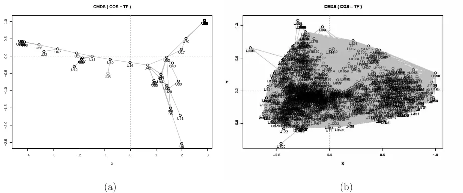
Figure 4: CMDS of simple (a) and complex network (b). While CMDS of 51 nodes (a) is scattered enough, CMDS of 1125 nodes (b) is complex.
Data Sets Documents Tags Used Remarks
[image:7.612.78.540.74.267.2]MSI-CIEC portal 92 178 d:51, t:86 In-house system Connotea 1131 6071 d:1125, t:4152 Harvested from Connotea
Table 2: Data sets used in the paper
so it is hard to be used for clusterings.
To overcome this problem, we devised a pre-process for relaxing complex relationships embedded in a tag graph. The intuition is to remove a weak edge if a node has more stronger one. For an example, let assume a nodedk having two edges with dissimilarityδik andδkj connecting to two nodesdianddj respectively. If
δik is much bigger than δkj (δik ≫δkj), we can ignore δik value by setting infinity. In our paper, we used
the following relaxation rule :
(
δik =∞, if δik·θ > δkj
δkj =∞, if δkj·θ > δik
, (2)
whereθ is a threshold factor ranged 0≤θ <1.
Results of relaxation will be explained in Section 3.
3
Experiments
The data used in this experiment is summarized in Table 2.
3.1
The graph model vs. the vector space model
We compared CMDS and Laplacian eigen map produced by using either the graph model (Figure 5(a) and 6(a)) or the vector space model (Figure 5(a) and 6(b)). We also compared the Q values for clustering quality measures. In order to observe the effectiveness of dimension reductions, we applied a clustering scheme (in this case we used hierarchical clustering algorithm [11]) to two cases: i) before dimension reduction (depicted as a dotted blue line in Figure 5 and 6) and ii) after dimension reduction(depicted as a solid lines in Figure 5 and 6). Note the solid lines. Depending on the data, the dimensions we can obtain from CMDS or Laplacian is from 1 up to the maximum number of positive eigen values of data. We computed exhaustively all Q
values for each possible dimensions from 2 up to the maximum.
We also computed CMDS or Laplacian for each use of TF, TF-IDF, COS, JAC, and PEA but the results are not vary. The summary of Q values are shown in Figure 7.
As a result, the graph based model is better than the vector space model. Overall, as shown in Figure 7, theQvalues based on the graph model (left pictures) are slightly bigger than ones based on the vector space model (right pictures). Also, the graphs show that the clustering with the data without dimension reduction is generally better. However, as seen in Figure 5(a), if we choose a right number of clusters, we can have better clustering efficiency according to Qvalues.
3.2
Complex Network Analysis
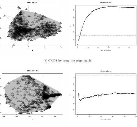
In the next experiment, we further investigated the usefulness of the graph model with high volume of data. We used the Connotea data in which over about 1100 nodes of document are connected with about 4100 tags. As observed in Figure 8, the CMDS graph shows the very complex structure. This implies the network of folksonomies as a complex network. Indeed, the network shows the scale-free network properties, which can be observed in many complex system, having lots of hub nodes with high degree of connections and so the length of the shortest path is relatively small. In our Connotea data, we observed that the maximum hop distance is only 4.
Anyway, although the CMDS graph looks so complex, the clustering qualityQshows better performance result. The Q values (the dark shaded bars) are even better than the Q values without using dimension reduction (lightly shaded bars). On the contrary, the Q values measured with the data using the vector space model shows poor performance.
3.3
Relaxation Effect
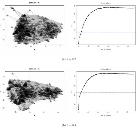
In this experiment, we have experimented to measure the effects of relaxation defined by Eq. 2 with Con-notea’s data in the graph model. For this purpose, we have applied our relaxation rule to the ConCon-notea’s data with respect to θ= 0.2 and 0.4 and measured clustering quality Qof CMDS (See Figure 10). As a result, comparing with no relaxation case as shown in Figure 8(a), clustering quality scores Qare increasing as θ
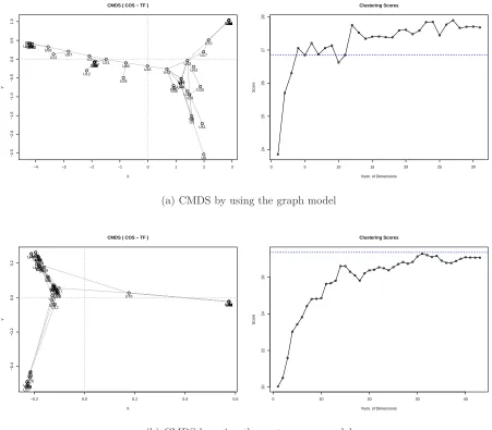
−4 −3 −2 −1 0 1 2 3 −2.5 −2.0 −1.5 −1.0 −0.5 0.0 0.5 1.0
CMDS ( COS − TF )
X Y U1 U2 U5 U6 U8 U10 U12 U13 U14 U16 U17 U21 U22 U26U27 U28 U29 U30 U31 U32 U41 U42 U43 U44 U46 U47 U50 U51 U52 U55 U56 U57 U58U61 U62 U64 U65 U66 U67 U68 U70 U71 U73 U74 U76 U79 U80 U82 U86 U87 U88
0 5 10 15 20 25 30
24 25 26 27 28 Clustering Scores
Num. of Dimensions
Score
(a) CMDS by using the graph model
−0.2 0.0 0.2 0.4 0.6
−0.4
−0.2
0.0
0.2
CMDS ( COS − TF )
X Y U1 U2 U5 U6 U8 U10
U12 U13U14
U16U17 U21 U22 U26 U27 U28 U29 U30U31 U32 U41 U42 U43 U44 U46 U47 U50 U51 U52 U55 U56 U57 U58 U61 U62 U64 U65 U66 U67 U68 U70 U71 U73 U74 U76 U79 U80 U82 U86 U87 U88
0 10 20 30 40
20
22
24
26
Clustering Scores
Num. of Dimensions
Score
[image:9.612.78.529.142.537.2](b) CMDS by using the vector space model
Figure 5: CMDS with MSI-CIEC data based on the graph model (a) and the vector space model (b). Both are using TF and COS. Q values for clustering quality is shown in the right. The horizontal blue dotted
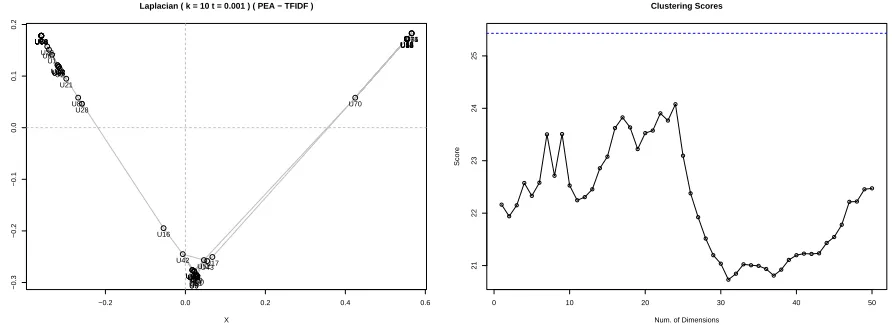
−0.2 0.0 0.2 0.4 0.6 −0.3 −0.2 −0.1 0.0 0.1 0.2
Laplacian ( k = 10 t = 0.001 ) ( PEA − TFIDF )
X Y U1 U2 U5 U6U8 U10 U12 U13 U14 U16 U17 U21 U22 U26U27 U28 U29U30 U31 U32 U41 U42 U43 U44 U46 U47 U50 U51 U52 U55 U56 U57 U58
U61 U62U64U65
U66 U67 U68 U70 U71 U73 U74 U76 U79 U80 U82 U86 U87 U88
0 10 20 30 40 50
21 22 23 24 25 Clustering Scores
Num. of Dimensions
Score
(a) Laplacian by using the graph model
−0.15 −0.10 −0.05 0.00 0.05
−0.10 −0.05 0.00 0.05 0.10 0.15
Laplacian ( k = 10 t = 0.001 ) ( PEA − TFIDF )
X Y U1 U2 U5 U6 U8 U10 U12 U13 U14 U16 U17 U21 U22 U26 U27 U28 U29 U30 U31 U32 U41 U42 U43 U44 U46 U47 U50 U51 U52 U55 U56 U57 U58 U61 U62 U64 U65 U66 U67 U68 U70U71 U73 U74 U76 U79 U80 U82 U86 U87 U88
0 10 20 30 40 50
20 21 22 23 24 25 26 Clustering Scores
Num. of Dimensions
Score
[image:10.612.82.528.144.312.2](b) Laplacian by using the vector space model
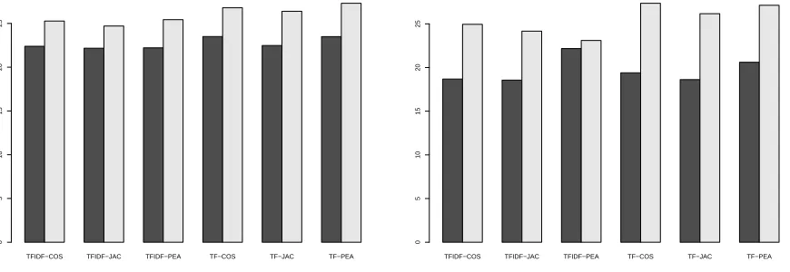
TFIDF−COS TFIDF−JAC TFIDF−PEA TF−COS TF−JAC TF−PEA
0
5
10
15
20
25
TFIDF−COS TFIDF−JAC TFIDF−PEA TF−COS TF−JAC TF−PEA
0
5
10
15
20
25
(a) CMDS with the graph model (left) and the vector space model (right)
TFIDF−COS TFIDF−JAC TFIDF−PEA TF−COS TF−JAC TF−PEA
0
5
10
15
20
25
TFIDF−COS TFIDF−JAC TFIDF−PEA TF−COS TF−JAC TF−PEA
0
5
10
15
20
25
[image:11.612.89.524.373.523.2](a) Laplacian with the graph model (left) and the vector space model (right)
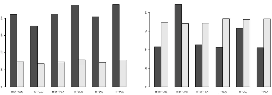
Figure 7: Qvalues for all experiments with MSI-CIEC data. Dark color bars represents the average of Q
values for all dimensions possible obtained from CMDS or Laplacian and the light color bar shows the Q
0 100 200 300 400 500
50
100
150
200
250
Clustering Scores
Num. of Dimensions
Score
(a) CMDS by using the graph model
0 100 200 300 400 500
20
30
40
50
60
70
Clustering Scores
Num. of Dimensions
Score
[image:12.612.83.533.128.543.2](b) CMDS by using the vector space model
Figure 8: CMDS with Connotea data based on the graph model (a) and the vector space model (b). Both are using TF and COS. Q values for clustering quality is shown in the right. The horizontal blue dotted
TFIDF−COS TFIDF−JAC TFIDF−PEA TF−COS TF−JAC TF−PEA
0
50
100
150
200
TFIDF−COS TFIDF−JAC TFIDF−PEA TF−COS TF−JAC TF−PEA
0
20
40
60
[image:13.612.86.520.86.238.2]80
Figure 9: Q values for clustering with/without using CMDS of Connotea data. The left picture is drawn based on the graph model and the right picture is based on the vector space model. Dark color bars represent the average ofQvalues for all dimensions possible obtained from CMDS and the light color bar shows the
Qvalues of clustering without dimension reduction. Clearly, the graph models show good performance than the vector space model.
4
Conclusion
In this paper, we investigated the two common model widely used in the field of information retrieval: the vector space model and the graph model. Although the vector space model is easy to use and can be directly applicable in the collaborative tagging systems, it has a disadvantage in describing the relationships which are commonly existing in folksonomy data. Contrary to the vector space model, the graph model is more suitable for the data in which members are highly inter connected and showing complex network structures. We verified this by performing clustering analysis and dimensional reduction schemes such as CMDS and Laplacian eigen map. In case of analyzing heavily entangled networks, we devised a relaxation scheme which can remove unrelated edges and help to improve clustering qualities for CMDS.
As for the future search, we are planning to apply more various clustering algorithms by using the graph model in order to drive more general conclusions.
References
[1] M. Belkin and P. Niyogi. Laplacian Eigenmaps for Dimensionality Reduction and Data Representation, 2003.
[2] K.W. Boyack, R. Klavans, and K. B¨orner. Mapping the backbone of science.Scientometrics, 64(3):351– 374, 2005.
[3] S. Deerwester, S.T. Dumais, G.W. Furnas, T.K. Landauer, and R. Harshman. Indexing by latent semantic analysis. Journal of the American Society for Information Science, 41(6):391–407, 1990.
0 100 200 300 400 500
50
100
150
200
250
Clustering Scores
Num. of Dimensions
Score
(a)θ= 0.2
0 100 200 300 400 500
50
100
150
200
Clustering Scores
Num. of Dimensions
Score
[image:14.612.73.536.138.575.2](b)θ= 0.4
[5] P. Gajer, M.T. Goodrich, and S.G. Kobourov. A Multi-dimensional Approach to Force-Directed Layouts of Large Graphs. Graph Drawing: 8th International Symposium Gd 2000, Colonial Williamsburg, Va, Usa, September 20-23, 2000: Proceedings, 2001.
[6] H. Halpin, V. Robu, and H. Shepherd. The complex dynamics of collaborative tagging. Proceedings of the 16th international conference on World Wide Web, pages 211–220, 2007.
[7] Y. Han. Efficient Parallel Algorithms for Computing All Pair Shortest Paths in Directed Graphs.
Algorithmica, 17(4):399–415, 1997.
[8] A. Noack. An energy model for visual graph clustering.Proceedings of the 11th International Symposium on Graph Drawing (GD 2003), LNCS, 2912:425–436.
[9] J.B. Tenenbaum, V. Silva, and J.C. Langford. A Global Geometric Framework for Nonlinear Dimen-sionality Reduction, 2000.
[10] J. Vesanto and E. Alhoniemi. Clustering of the self-organizing map. Neural Networks, IEEE Transac-tions on, 11(3):586–600, 2000.