Audio coding: 3-dimensional stereo and presence

3-dimensional stereo and presence

Audio coding

Scheme: CIN / TIS / M.Eng.

Version: 1.0

Last update: January 2002

Date: January 2002

2

Introduction

In this second lecture, we will examine the design and operation of audio codecs. An audio codec is a device that reduces the amount of data required to represent an audio signal. We will discuss the need for audio coding, the general principles of audio coding, and the design of a phychoacoustic model.

2.1

Why reduce the data rate?

The compact disc is now so much a part of everyday life that its technological properties are taken for granted. Indeed, the 750 MB of audio data contained upon a typical CD seems small compared to the capacity of current storage devices. Moore’s law [1] predicts that computational processing power will double every 18 months. Data storage capacity is increasing at a similar rate. The capac-ity of the humble CD will seem minuscule compared to next year’s hard disk drives and future optical disc formats.

As the storage capacity of a CD is dwarfed, it is easy to forget that the data requirements of CD quality digital audio are immense compared to textual media. For example, 30 seconds of CD qual-ity digital audio requires the same storage space as the complete works of Shakespeare1_{. Though the}

cost of digital storage falls year on year, the data rate of CD quality audio is still too high for certain applications. Two pertinent examples are discussed below.

Firstly, audio broadcasters wish to transmit CD quality radio services. However, the radio spectrum is very crowded, and the proliferation of devices such as mobile phones has made radio bandwidth an expensive commodity. If CD quality audio were transmitted on existing analogue FM frequen-cies, then the frequency range from 88 MHz to 108 MHz would accommodate just 12 radio stations. However, analogue transmissions must continue during the transition to digital broadcasting, so additional bandwidth has been allocated for the digital services2. The bandwidth allocated for the five BBC national radio stations is 1.54 MHz. After channel coding, this yields a broadcast data rate of 1.2 Mbps. The data rate of CD is 1.4 Mbps. Thus, a single CD-quality audio service requires more bandwidth than is available for five radio stations.

Secondly, computer networks, especially home connections, have failed to increase in capacity in accordance with Moore’s law. The most common internet connection at home in the UK is cur-rently the 56k modem. Data transfer rates of approximately 3-4 KB per second (32000 bits per second) are typical. Thus, for every one second download time, the user can transfer 0.0227 seconds of CD quality audio. Real-time delivery of audio in this manner is impossible. Distributing albums of music over the internet for off-line listening is similarly impractical, since a 3 minute pop song requires over two hours download time.

1 _{The complete works of Shakespeare in ASCII Plain text format occupy 5219KB, or 44153344 bits. 30 seconds of CD}

quality audio occupy 44100*16*2*30=42336000 bits. Thus this edition of the complete works of Shakespeare requires the same binary storage as 31.3 seconds of CD quality digital audio.

2 _{In the United Kingdom, 12.5 MHz of Band III spectrum from 217.5 - 230 MHz has been allocated to digital audio}

broadcasting. This will accommodate seven data channels. The BBC has been allocated one of these channels for its national services.

The data rate of CD quality digital audio is too high for both these applications. The data rate must be reduced in order to make either application practical. In addition, there are other applications where the data rate of CD quality audio is not prohibitive, but reducing this data rate would provide economic or functional benefits. For these reasons, it is desirable to reduce the data rate of the audio signal, without compromising the audio quality. However, without sophisticated audio codecs, the data rate and audio quality are inextricably linked.

2.2

Data reduction by quality reduction

The simplest method of reducing bitrate3 is to reduce the audio quality. Three bitrate reducing strategies are listed below, together with the quality implications for each strategy.

1. Reduce the sampling rate. This will reduce the frequency range (bandwidth) of the audio signal. 2. Reduce the bit-depth. This will increase the noise floor of the audio signal.

3. Convert a stereo (2-channel) signal to a mono (1-channel) signal. This will remove all spatial information from the audio signal.

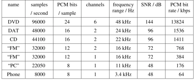
Table 2.1 lists some common audio formats. These illustrate various combinations of the above strategies.

The lowest bitrate in Table 2.1 is still too high to transmit in real time over a 56k modem. The stereo “FM” parameters define a digital channel with comparable quality to existing analogue FM broadcasts. This quality is acceptable to most consumers, but quality reductions below this level are perceived and disliked by many listeners.

To reduce the bitrate further, a more sophisticated approach is required.

3 _{Throughout this discussion, the data rate of an audio signal will be referred to as the “bitrate”. The bitrate is specified}

in bits per second (bps), kilobits per second (kbps), or Megabits per second (Mbps). The “k” and “M” prefixes are used to represent 103 _{and 10}6 _{respectively (SI units) rather than 2}10 _{and 2}20 _{(commonly used in PC specifications - see [IEC}

name samples / second

PCM bits / sample

channels frequency

range / Hz SNR / dB rate / kbpsPCM bit

DVD 96000 24 6 48 kHz 144 13824 DAT 48000 16 2 24 kHz 96 1536 CD 44100 16 2 22 kHz 96 1411 “FM” 32000 12 2 16 kHz 72 768 “FM” 32000 12 1 16 kHz 72 384 “PC” 22050 8 1 11 kHz 48 176 Phone 8000 8 1 3.4 kHz 48 64

2.3

Lossless and lossy audio codecs

There are two distinct types of audio codec: lossless and lossy. A lossless codec will return an exact copy of the original digital audio signal following the encode and decode process. A similar ap-proach is often used within the computer world to reduce the size of documents or program files, without changing the data. Algorithms suitable for data include “Zip” [2] and “Sit” [3]. Algorithms suitable for audio include “LPAC” [4], “Meridian Lossless Packing” (MLP) [5], and “Monkey’s Audio” [6]. Both types of algorithm exploit redundancies within the data. For example, the wav e-forms of musical signals are often repetitive in nature. Storing the difference between each cycle of the waveform, rather than the waveform itself, often requires fewer bits. In a lossless codec, the difference between the predicted values and the actual waveform is also stored, so that the wave-form can be reconstructed exactly. Further details of lossless codec design are given at the end of these notes.

A lossless audio codec by definition cannot reduce the audio quality. However, lossless audio codecs rarely reduce the bitrate to below 50% of the original value. Also, the exact bitrate reduction is highly signal dependent, so the bitrate of the audio data cannot be guaranteed to match that of the transmission channel. A burst of white noise (which is random and hence difficult to predict or compress) may cause the encoded bitrate to match or exceed that of the original signal.

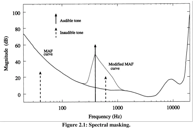
To reduce the bitrate still further, lossy audio codecs discard audio data. This means that the de-coded waveform is not an exact copy of the original. However, unlike the measures described in 2.2, lossy audio codecs aim to discard data in a manner that is inaudible, or at least not objection-able to a human listener. This is possible due to the complex nature of human hearing. This topic was discussed in depth in the first lecture. To summarise: the presence of one sound can prevent a human listener from hearing a second (quieter) sound. This phenomenon is illustrated in Figure 2.1 [7]. The MAF curve represents the level below which a sound of a given frequency is inaudible. The presence of an audible tone raises the threshold in the spectral region around the tone, such that any additional sound falling below the masked threshold (as indicated in Figure 2.1) is inaudible.

Where this occurs, the masked sound can be removed or distorted by the audio codec without changing the perceived quality of the audio signal. Lossy codecs which operate in this manner are often referred to as psychoacoustic based codecs, since they require knowledge of the properties of the human auditory system.

By combining this approach with lossless data reduction, the bitrate may be reduced by 90% with-out significantly reducing the perceived audio quality. The result is that a bitrate which provides little better than telephone quality without data reduction, can yield near CD quality with data re-duction.

Psychoacoustic based codecs are the most recent generation of lossy audio codecs. Two other types or families of lossy audio codec exist, and these are mentioned in passing. The first type aims to discard data without significantly reducing the perceived quality of the audio signal, but does so without sophisticated knowledge of the human auditory system. The oldest such codecs are the A-law and µ-law coding schemes, where non-linear quantisation steps are used to increase the per-ceived signal to noise ratio of an 8-bit quantiser.

Another lossy coding mechanism is Adaptive Differential Pulse Code Modulation. In ADPCM, each sample is predicted from the previous samples, and only the difference between the prediction and the actual value is stored. The decoder follows the same predictive rules as the encoder, and adds the stored difference to each predicted sample value. Typically, the input samples are of 8 or 16 bit resolution, and the encoded differences are stored in four bit resolution, giving 50% or 75% data reduction. This codec is lossless, except where the difference between the predicted and actual values cannot be represented in four bits. In practice, this situation is common, but the error is sometime inaudible, and rarely annoying.

Both the above lossy codecs are designed for use with telephone quality speech signals, though they can be used with some success to code CD quality music signals. There is a further type of lossy codec which is designed for speech coding only. Code excited linear predictive coding employs a code book of excitation signals followed by a linear predictive filter. The output of the code book and filter is compared with the incoming speech signal, and the code book index which gives the best match is transmitted. Typically, a single 10-bit index into the code book can represent 40 in-coming samples. This mechanism of lossy coding is used on digital mobile telephone networks, and the code book is designed to represent speech-like sounds. This approach is not suitable for high quality music coding, as anyone who has heard music via a GSM mobile phone can testify. These speech-only lossy codecs are not relevant to the high quality audio, and will not be discussed fur-ther.

Psychoacoustic based lossy codecs are most relevant to high quality audio. The general principle of operation, and the details of the popular MPEG-1 family of codecs will now be discussed.

2.4

General psychoacoustic coding principles

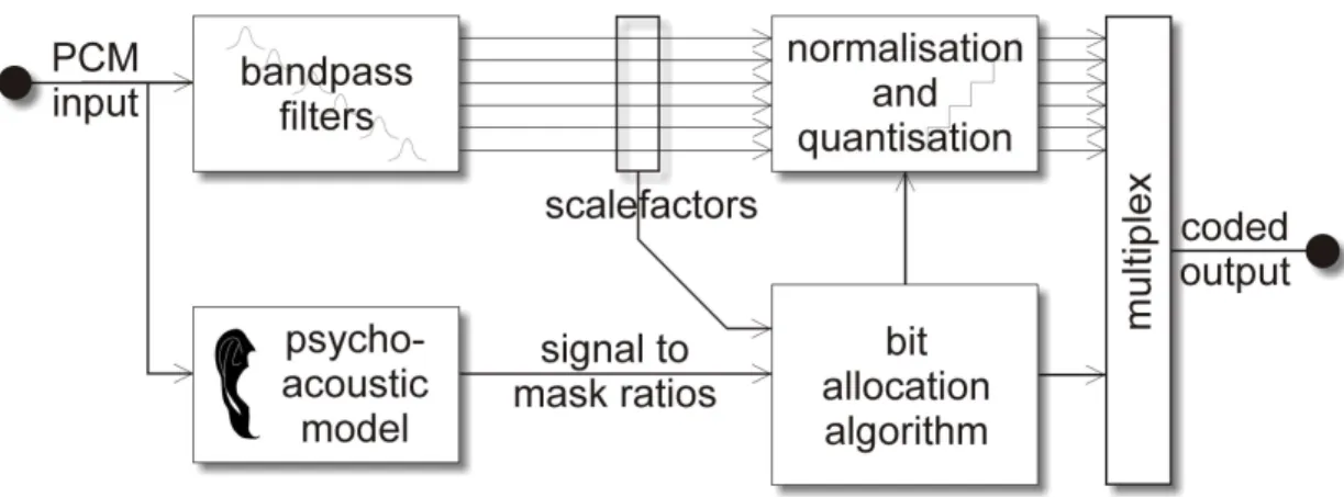
A generalised psychoacoustic codec may operate as shown in Figure 2.2. In the first stage of the encoder, the incoming signal is split into several frequency bands by a bank of bandpass filters. A psychoacoustic model calculates the masked threshold for each frequency band, and this is con-verted into a Signal to Mask Ratio for each band. Spectral components that lie above the masked threshold are judged to be audible, and yield a positive Signal to Mask Ratio. Spectral components that lie below the masked threshold are judged to be inaudible, and yield a negative Signal to Mask Ratio.

The Signal to Mask ratio directs a bit allocation algorithm. The number of bits allocated to each frequency band determines the accuracy of the quantiser, which in turn determines the amount of noise that will be added within each band. The intention is to add noise within masked spectral regions of the audio signal, but not to change or distort audible spectral components.

The amplitude of the signal in each band is normalised to unity before quantisation, and the scale factor required to revert the signal to its original level is stored, along with the output of the quan-tiser. The scale factor and/or quantiser output for a given band may be omitted if the signal within

the frequency band lies well below the masked threshold. The resulting bitrate is much less than that of the original audio signal.

The decoder reverses this process by generating the signal in each band from the quantised values, multiplying each signal by the appropriate scale factor, and bandpass filtering the contents of each band. Finally, outputs of all the frequency bands are summed to yield the final decoded audio sig-nal. Hopefully, the decoded signal will sound almost identical to the original sigsig-nal.

The accuracy of the psychoacoustic model will effect the perceived sound quality of the coded audio. If the model incorrectly predicts that a spectral component is inaudible, when in reality is it above the masked threshold, then a human listener will perceive the noise added by the codec within this frequency region. However, even if the psychoacoustic model perfectly predicts human perception, the resulting coded audio signal will still contain audible noise if the bitrate is too low. In a constant bitrate compressed audio signal, only a certain number of bits are available per second. If the psychoacoustic model calculates a high Signal to Mask Ratio for many frequency bands, this may instruct the bit allocation model to use more bits than are available. In this case, the bit alloca-tion model must choose the best compromise to minimise the audible coding noise, whilst remaining within the allocated bitrate. Variable bitrate coding overcomes this problem, by allocat-ing the correct number of bits to ensure that the quantisation noise within each frequency band is below the masked threshold. This will reduce the bitrate during quiet or easy to encode passages, whilst increasing the bitrate during loud or complex passages. Variable bitrate encoding is only available within some audio codecs.

There are two sub-types of psychoacoustic codec: subband codecs and transform codecs. Subband codecs store the waveform present in each frequency band in a sub-sampled, quantised form. Trans-form codecs perTrans-form a time to frequency transTrans-formation (e.g. the Fast Fourier TransTrans-form) upon the original audio signal, or the signal within each frequency band. The resulting transform coefficients are stored, after quantisation, according to the SMR prediction of the psychoacoustic model. Trans-form codecs typically offer greater bitrate reduction than subband codecs. This is partly due to the higher frequency resolution offered by the transform, which allows the coding noise to be distrib-uted more accurately according to the masked threshold. The major disadvantage of transform coding is that all current time to frequency transformations process the audio in discrete time do-main blocks, and this blocking can cause audible problems. These problems will be discussed in Section 2.5.3, with respect to the MPEG-1 layer III codec.

2.5

MPEG audio codecs

These general principles of audio coding are seen at work in the MPEG-1 family of audio codecs. The MPEG-1 standard consists of three “layers” of coding, where each layer offers an increase in complexity, delay, and subjective performance with respect to the previous layer. The higher layers build on the technology of the lower layers, and a layer n decoder is required to decode all lower layers. The MPEG-1 standard [8] supports sampling rates of 32 kHz, 44.1 kHz and 48 kHz, and bitrates between 32 kbps (mono) and 448 kbps (Layer I stereo). The MPEG-2 standard [9] contains a backwards compatible multi-channel codec, and extends the range of allowed bitrates and

sam-pling rates4. A proprietary extension called MPEG-2.5 [10] is in common use for layer III. The sampling rates and bitrates are summarised in the following table.

A review of the MPEG standards for audio coding is found in [11], and a clear description of layer III and AAC coding is contained in [12]. Parts of the following explanation are drawn from [13].

4 _{The MPEG-2 standard also defines a non-backwards compatible codec known as MPEG-2 AAC (Advanced Audio}

Coding). This section of the standard was finalised some years after layers I, II, and III. It includes several refinements that improve coding efficiency (most notably temporal noise shaping), but the general coding principles are very similar to MPEG-1 layer III. Further details can be found in the standards document and an excellent description appears in [Bosi et al, 1997]. codec sampling rates / kHz allowed bitrates / kbps MPEG-1 layer I 32, 64, 96, 128, 160, 192, 224, 256, 288, 320, 352, 384, 416, 448 layer II 32, 48, 56, 64, 80, 96, 112, 128, 160, 192, 224, 256, 320, 384 layer III 32, 44.1, 48 32, 40, 48, 56, 64, 80, 96, 112, 128, 160, 192, 224, 256, 320 MPEG-2 layer I 32, 48, 56, 64, 80, 96, 112, 128, 144, 160, 176, 192, 224, 256 layer II 8, 16, 24, 32, 40, 48, 56, 64, 80, 96, 112, 128, 144, 160 layer III 16, 22.05, 24 8, 16, 24, 32, 40, 48, 56, 64, 80, 96, 112, 128, 144, 160 MPEG-2.5 layer III 8, 11.025, 12 8, 16, 24, 32, 40, 48, 56, 64, 80, 96, 112, 128, 144, 160

2.5.1

MPEG-1 layer I audio coding

The structure of the MPEG-1 layers I and II encoder is shown in Figure 2.3.

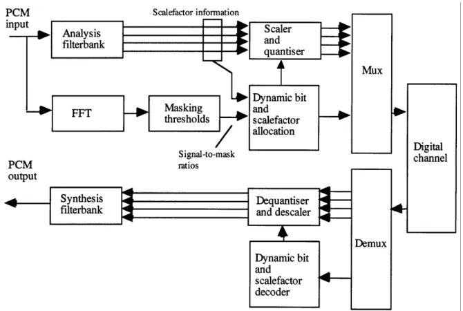
The operation of the layer I encoder is as follows. All references to time and frequency assume 48 kHz sampling.

1. The analysis filterbank splits the incoming audio signal into 32 spectral bands. The filters are

linearly spaced, each having a bandwidth of 750 Hz.

2. The samples in each band are critically decimated, and split into blocks of 12 decimated

sam-ples. Scalefactors are calculated which normalise the amplitude of the maximum sample in

each band to unity.

3. In a parallel process, the signal is windowed, and a 512-point FFT is performed, to calculate

the spectrum of the current audio block.

4. The psychoacoustic model calculates the masked threshold from the spectrum of the current

block. This is transformed into a Signal to Masker Ratio for each band.

5. The dynamic bit and scalefactor allocator selects one of 15 possible quantisers for each band,

based upon the available bitrate, the scalefactor, and the masking information. The aim is to meet the bitrate requirements whilst masking the coding noise as much as possible.

6. The scaler and quantiser acts as instructed by the allocator, to scale and quantise each block of

12 samples.

7. Finally, the quantised samples, scalefactors, and control information are multiplexed together

for transmission or storage.

The decoder unpacks this information, scales and interpolates the quantised samples as instructed

via the control information, and passes the 32 bands through a synthesis filter to generate PCM audio samples. The decoder does not require a psychoacoustic model, so decoder complexity is reduced compared to the encoder. This is useful for broadcast applications, where a single (expen-sive) encoder must transmit to thousands of (inexpen(expen-sive) decoders.

The decoder is specified exactly by the MPEG standard, but the encoder can use any coding strat-egy that yields a valid bitstream. For example, the psychoacoustic model may be arbitrarily complex (or non-existent if encoding speed is the only concern). In theory, this allows future devel-opments in psychoacoustic knowledge to be incorporated into the encoder, without breaking compatibility with existing decoders. In practice, the fixed choice of filterbank parameters limits the fine-tuning that may be carried out.

2.5.2

MPEG-1 layer II

The layer II codec operates in a similar manner to layer I, but achieves higher audio quality at a given bitrate via the following modifications.

1. The 512-point FFT is replaced by a 1024-point FFT. This increases the frequency resolution of the masking calculation, at the expense of increasing the encoder delay.

2. The similarity between adjacent scalefactors in adjacent blocks is exploited, thus reducing the amount of control information that must be transmitted.

3. More accurate (smaller stepped) quantisers are made available.

MPEG-1 later II coding is used by Digital Audio Broadcasting within the UK and much of the world (apart from America). It achieves near CD-quality at around 256 kbps stereo.

2.5.3

MPEG-1 layer III

The layer III codec is significantly more complex than the lower layers. It uses both subband and transform coding, and is the only layer with mandatory support for variable bitrate coding. The layer III encoder is shown in Figure 2.4.

Each of the 32 frequency bands is sub-divided by a 6-point or 18-point Modified Discrete Cosine Transform. This gives a possible frequency resolution of up to 42 Hz, compared to 750 Hz for layers I and II. The layer III codec switches between the two possible MDCT lengths (often referred to as short and long blocks) depending on the input signal. This strategy is useful because, after quantisation of the coefficients, the temporal structure of the audio information within the MDCT block is often distorted. Hence, short blocks are used for encoding transient information to minimise audible temporal smearing, while long blocks are used for near steady-state signals to give in-creased spectral accuracy.

Three other significant improvements are included in the layer III encoder. A non-uniform quantiser is used to increase the effective dynamic range (in a similar manner to A-law or µ-law encoding, but operating upon a single frequency band). The quantised samples are losslessly packed using Huffman coding. Finally, a bit reservoir is included in the layer III specification. This allows the encoder to increase the bitrate during brief “hard to encode” sections, so long as it can reduce the bitrate during a nearby “easy to encode” section. The overall bitrate is held constant, so the scheme is still referred to as “constant bitrate”. In this manner, the reservoir provides some of the adva

tages of variable bitrate coding, whilst maintaining compatibility with fixed bitrate transmission channels.

The layer III decoder is more complex than that required for layers I or II. However, the popularity of MPEG-1 and -2 layer III has led to low-cost single chip layer III decoders becoming available. Layer III is said to offer near CD quality at 128 kbps.

Many of the intricacies of the MPEG-1 layers are not covered here. Example encoders and decoders are described in the appropriate standards documents ([8] and [9]). One important feature is dis-cussed in the next section.

2.5.4

Joint stereo coding

The redundancy sometimes found within two channel (stereo) signals allows for a significant bitrate reduction without a corresponding reduction in audio quality. MPEG-1 defines four modes:

1. Mono 2. Stereo

3. Dual (two separate channels) 4. Joint Stereo

In the first three modes, one or two separate channels are coded individually. In the fourth mode, the information in the two stereo channels is combined in one of two possible ways to reduce the bitrate.

Intensity stereo coding takes advantage of the human ear’s insensitivity to interaural phase diffe

r-ences at higher frequencies.

For each frequency band, the data from the two stereo channels is combined, and the resulting single channel of audio data is coded. Two coefficients are also stored to define the level at which this single channel should appear in each of the stereo channels upon decoding. This procedure is only appropriate at higher frequencies, but it can offer a 20% bitrate saving compared to normal stereo. Unfortunately, the use of intensity stereo can be audible. Though the ear cannot detect the interaural phase of high frequency tones, the ear can detect interaural time delays in the envelope of high frequency signals. These time delays are destroyed by intensity stereo coding, and the stereo image appears to partially collapse. However, this effect is less objectionable than highly audible coding noise, so intensity stereo is useful at low bitrates, where it effectively frees some bits to reduce the coding noise.

Matrix stereo coding exploits the similarity between two stereo channels. Rather than coding the

Left and Right Channels, the Sum (or “Middle”) and Difference (or “Side”) signals are coded i n-stead, thus: 2 R L M = + _(2-1) 2 R L S = − _(2-2) 2 S M L= + _(2-3) 2 S M R= − _(2-4)

The transformation from L/R to M/S is entirely lossless and reversible via equations (2-3) and (2-4), though quantisation of the M/S signals will prevent perfect reconstruction in practice. For a signal with very little difference between the two stereo channels (i.e. an “almost” mono signal) the energy within the S channel is minimal, and the bitrate required for this channel is comparatively low. Thus, for a mono or 100% out of phase signal, the bitrate reduction is nearly 50%. For most audio signals, some bitrate reduction may be achieved by the use of joint stereo. It offers no benefit where the two stereo channels are completely uncorrelated. In some circumstances, it may cause problems. For example, consider a stereo signal consisting of audio on the left channel only, with an almost silent right channel. The right channel may contain a hiss, or a quiet echo. The M and S channels will be almost identical. However, the difference between the two channels is enough to ensure that the coding noise introduced into each channel is not identical. This coding noise is masked in both channels of the M/S representation. When the left and right channels are restored in the decoder, the right channel consists of the difference between the M and S signals. Hence, the right channel will contain very little signal information, but lots of coding noise. This occurs because the signal that masked the coding noise in the M/S representation is spatially separated from the coding noise in the decoded L/R output.

MPEG-1 layer III can use a combination of stereo techniques, in which the encoder switches dy-namically between independent stereo, matrix stereo, and/or intensity stereo, depending on the incoming audio signal and the desired bitrate. This is yet another reason why layer III can achieve higher quality at a specified bitrate, or a lower bitrate at a given quality than layers I and II.

It is interesting to note the target bitrates of the three layers. The specifications suggest that layers I and II achieve CD quality at 256 kbps stereo; layer II at 192 kbps joint stereo, and layer III at 112-128 kbps joint stereo. Experience suggests that these recommendations are less than exact. Some audio signals are audibly degraded by some or all of the layers at any bitrate. Further, the suggested bitrate for layer III is especially optimistic; nearly twice this bitrate is often required to ensure CD

16 kHz at 128 kbps, which is by definition not CD quality. Whilst many audio extracts do sound acceptable at 128 kbps, a significant minority do not.

3

The Psychoacoustic model

One of the most important components within a pyschocacoustic based codec is the psychoacoustic model. This consists of an algorithm that predicts what is (and is not) audible to a human listener. In theory, the sound quality of an audio codec depends on the accuracy of the psychoacoustic model within the encoder. In practice, other factors are equally as important as the psychoacoustic model, such as the filterbank parameters and the choice of block-size. If the rest of the codec is well de-signed, then a comparatively simple psychoacoustic model can yield good results. A basic psychoacoustic model will be described here.

In 1988, James Johnston published details of a model for calculating the “perceptual entropy” of audio signals [14]. This model calculates the masked threshold due to an audio signal in order to predict which components of the signal are inaudible. In this way, the model can be used to predict how much data is needed to transparently code the signal. The model is included in an audio coder [15], where the prediction of inaudible components is used to feed a bit allocation algorithm which reduces the data rate to 128 kbps for a mono signal. Similar models are included in most audio codecs.

The Johnston model calculates the spectral masking due to an audio signal, but temporal masking is not addressed. Though the human auditory system is continuous in both time and frequency, the spectral masking estimate calculated by the Johnston model is discrete in time and frequency. The signal is split into short (64 ms) frames, and the spectral masking for each frame is computed as if the signal were steady state. The masking is computed for 25 frequency bins, spaced equally on the critical band scale. Thus one masked threshold is calculated for each frequency bin every 64 ms. This threshold is calculated by taking the FFT of a 64 ms frame, summing the energy in each fre-quency bin, spreading the energy to simulate spectral masking, adjusting for the nature of the signal, and normalising the result.

The following detailed walk through the Johnston auditory model is drawn from [14], [15], and [7]. The plots show the progress of a synthetic signal (consisting of a 500Hz tone and a 5kHz tone) through the model.

3.1

Algorithm

3.1.1

Window and FFT

The audio signal is split into frames. A frame length of 64ms is employed (2048 samples at a sampling frequency of 32kHz).

The current frame is windowed with a Hanning (raised cosine) window and an FFT (Fast Fourier Transform) is performed. Each line (n) in the com-plex FFT refers to a spectral component of frequency

f (in kHz), given by window f l n f s * 1000 . ) ( = , (3-1)

which is valid for the first (window/2) complex lines.

3.1.2

Critical Band Analysis

The real and imaginary components of the spectrum Re(n),Im(n)from the FFT are converted to the power spectrum, P(n), thus:

) ( Im ) ( Re ) (_n 2 _n 2 _n P = + (3-2)

This power spectrum is segregated in linear frequency, but the auditory system processes frequency on a near logarithmic scale, called the critical band scale, as discussed in the first lecture. The rela-tionship between linear frequency, f in kHz, and the critical band, or Bark frequency, zcin Bark, is given by

(

)

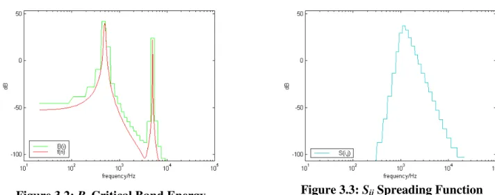
adapted from [16] to number critical bands from 1 to 25. If the lowest frequency component falling in critical band i, where i=int(zc), is given by bli, and the highest frequency component falling in critical band i is given by bhi, then the summation of the energy in band i is given by:

∑

The energy in each critical band is summed in this manner. The D.C. component of the spectrum is not included in this summation.

3.1.3

Spreading function

The following spreading function (taken from [17]) is used to estimate the effects of masking across critical bands.

(

)

(

)

y = i− j (not the modulus, as stated in some other papers)

i = Bark frequency of masked signal j = Bark frequency of masker signal

The spread critical band spectrum is calculated by convolving the spreading function with the critical band spectrum. This can be achieved by matrix mul-tiplication, thus:

Figure 3.2: Bi Critical Band Energy Figure 3.3: Sij Spreading Function

                ×                 =                 25 3 2 1 25 , 25 3 , 25 2 , 25 1 , 25 25 , 3 3 , 3 2 , 3 1 , 3 25 , 2 3 , 2 2 , 2 2 , 1 25 , 1 3 , 1 2 , 1 1 , 1 25 3 2 1 ... ... ... ... ... ... ... ... ... ... ... B B B B S S S S S S S S S S S S S S S S C C C C (3-7)

3.1.4

Coefficient of tonality

The masking threshold for noise masked by a tone is taken to be 14.5+i dB below Ci, but the masking threshold for a tone masked by noise is taken to be 5.5 dB below Ci [15]. Johnston uses the Spectral Flatness Measure (SFM), calculated from the geometric and arithmetic means of the power spectrum, to determine how tone-like or noise-like the signal is. The SFM is given by

( )

( )

(

)

∑

∑

and N =window/2. An SFM of zero dB would indicate that the signal is entirely noise like, while

an SFM >=SFMdB_max, where SFMdBmax =−60dB, would indicate that the signal is entirely tone

like. Most tone like signals, such as organ, sine waves, or flute have an SFM that is close to or over the limit. A coefficient of tonality is calculated as follows:

    =min ,1 max dB dB SFM SFM α (3-11)

This coefficient is used to geometrically weight the two thresholds, yielding Oi, the threshold off-set, thus: 5 . 5 ) 1 ( ) 5 . 14 ( α α + + − = i Oi (3-12)

3.1.5

Spread threshold estimate

The offset Oi is subtracted from the spread critical band spectrum Ci to give the spread spectrum esti-mate Ti, thus: ) 10 / ( ) ( log10 10 Ci Oi i T ₌ − _(3-13)

3.1.6

Re-normalisation of the threshold

es-timate

The spreading function described in Section 3 in-creases the overall energy, where as the psychophysi-cal process that we are attempting to model spreads the energy by dispersing it. For example, examine the behaviour with a hypothetical stimulus with unity energy in each critical band. The actual spreading function of the ear will result in no overall change to the level of energy in any critical band5. However, the spreading function presented here will cause the energy in each band to increase, due to the additive contributions of energy spread from adjacent critical bands.

The solution presented here is to normalise the threshold estimate at this stage. A hypothetical stimulus, with unity energy in each critical band, is used as the Bi in equation (3-7), to give the spread spectrum error, CEi, thus:

                ×                 =                 1 ... 1 1 1 ... ... ... ... ... ... ... ... ... ... 25 , 25 3 , 25 2 , 25 1 , 25 25 , 3 3 , 3 2 , 3 1 , 3 25 , 2 3 , 2 2 , 2 2 , 1 25 , 1 3 , 1 2 , 1 1 , 1 25 3 2 1 S S S S S S S S S S S S S S S S C C C C E E E E (3-14)

The normalised threshold estimate '

i

T is calculated by converting CEi into dB, and subtracting it from the threshold estimate, thus:

5 _{In reality the lowest and highest bands will loose energy by this process, but all other bands will loose and gain equal}

amounts of energy by dispersion, hence the total level of energy in each band will remain unchanged.

Figure 3.5: TI Spread Threshold

Estimate

Figure 3.6: Ti′′

( )

i T C

T'_{= −10log10 (3-15)}

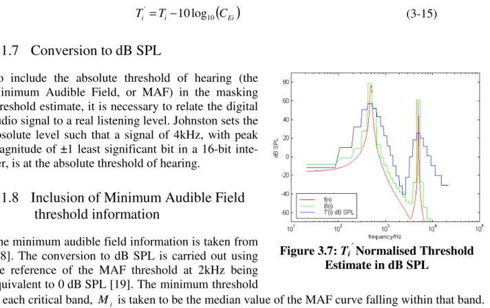
3.1.7

Conversion to dB SPL

To include the absolute threshold of hearing (the Minimum Audible Field, or MAF) in the masking threshold estimate, it is necessary to relate the digital audio signal to a real listening level. Johnston sets the absolute level such that a signal of 4kHz, with peak magnitude of ±1 least significant bit in a 16-bit inte-ger, is at the absolute threshold of hearing.

3.1.8

Inclusion of Minimum Audible Field

threshold information

The minimum audible field information is taken from [18]. The conversion to dB SPL is carried out using the reference of the MAF threshold at 2kHz being equivalent to 0 dB SPL [19]. The minimum threshold

in each critical band, Mi is taken to be the median value of the MAF curve falling within that band. Hence, the final threshold estimate is given by

(

)

This estimate is compared to the signal level in each band, and a signal to masker ratio is calculated. The SMR drives the bit allocation algorithm, as described in section 2.5.1.

Figure 3.7: Ti′′ Normalised Threshold

Estimate in dB SPL

4

Lossless audio coding

The following explanation of lossless audio coding was written by Matt Ashland, and is reproduced with permission. See http://www.monkeysaudio.com/theory.html for more details.

4.1

Conversion to X,Y

The first step in lossless compression is to model the channels L and R in a more efficient manner, as some X and Y values. There is often a great deal of correlation between the L and R channels, and this can be exploited several ways, with one popular way being through the use of mid / side encoding. In this case, a mid (X) and a side (Y) value are encoded instead of a L and a R value. The mid (X) is the sum of the L and R channels and the side (Y) is the difference in the channels. This can be achieved, thus:

X = (L + R) / 2 Y = (L - R)

4.2

Predictor

Next, the X and Y data is passed through a predictor in an attempt to remove any redundancy. The aim of this stage is to make the X and Y arrays contain the smallest possible values while still re-maining decompressible. This stage is what separates one compression scheme from another. There are virtually countless ways to do this. Here is a sample using simple linear algebra:

PX and PY are the predicted X and Y; X-1is the previous X value; X-2 is the X value two back

PX = (2 * X-1) - X-2 PY = (2 * Y-1) - Y-2

As an example, if X = (2, 8, 24, ?); PX = (2 * X-1) - X-2 = (2 * 24) - 8 = 40

Then, these predicted values are compared with the actual value and the difference (error) is what gets sent to the next stage for encoding.

Most good predictors are adaptive, i.e. that they adjust to how “predictable” the current data is. For example, consider a factor 'm' that ranges from 0 to 1024 (0 is no prediction and 1024 is full predi c-tion). After each prediction, m is adjusted up or down depending on whether the prediction was helpful or not. Therefore, in the previous example, the output of the predictor is:

X = (2, 8, 24, ?)

PX = (2 * X-1) - X-2 = (2 * 24) - 8 = 40

If ? = 45 and m = 512, then [Final Value] = ? - (PX * m / 1024) = 45 - (40 * m / 1024) = 45 - (40 * 512 / 1024) = 45 - 20 = 25

After this sample, m would be adjusted upwards because a higher m would have been more effi-cient.

Using different prediction equations and using multiple passes through the predictor can make a substantial difference in the compression ratio that may be achieved. Here is a list of some predic-tion equapredic-tions as shown in the Shorten technical documentapredic-tion [20] (for different orders):

P0 = 0 P1 = X-1

P2 = (2 * X-1) - X-2

P3 = (3 * X-1) - (3 *X-2) + X-3

4.3

Encoding of Data / Rice coding

The goal behind audio compression is to make all of the numbers as small as possible by removing any correlation that may exist between them…once this is achieved the resulting numbers must be written to disk. One of (if not the) most efficient way to do this is with rice coding.

Why are smaller numbers better? They are better because they can be represented using fewer bits. For example, consider the following array of numbers (32 bit longs):

Base 10: 10, 14, 15, 46 or, in binary: Base 2: 1010, 1110, 1111, 101110

Now obviously if we want to represent these numbers in the fewest possible bits, it would be quite inefficient to represent them each as separate longs with 32 bits apiece. That would take 128 bits, and just from looking at the same numbers represented in base two, it is obvious that there must be a better way. The ideal thing would be just to concatenate the four numbers together using the least bits necessary, so 1010, 1110, 1111, 101110 without the commas would be 101011101111101110. The problem here is that we don't know where one number starts and the next begins. This is where rice coding comes into play.

Rice coding is a way of using fewer bits to represent small numbers, while still maintaining the ability to tell one from the next. In essence, it works as follows:

1) Make a best guess as to how many bits a number will take, and call that k 2) Take the rightmost k bits of the number and remember what they are

3) Imagine the binary number without those rightmost k bits and look at its new value (this is the overflow that doesn't fit in k bits)

4) Use these values to encode the number; This encoded value is represented as a number of zeroes corresponding to step 3, followed by a 1 to terminate the "overflow", then finally the k bits from step 2.

1) You make your best guess as to how many bits a number will take, and call that k: since the previous 3 numbers took 4 bits, that seems like a reasonable guess so we will set k = 4

2) Take the rightmost k bits of the number and remember what they are: The right 4 bits of 46 (101110) are 1110

3) Imagine the binary number without those rightmost k bits and look at its new value (this is the overflow that doesn't fit in k bits): When you take the 1110 away from the right of 101110 you are left with 10 or 2 (in base 10)

4) Use these values to encode the number… So, we put two 0's, followed by the terminating 1, followed by the k bits 1110…altogether we have 0011110

To reverse this operation, we just take 0011110 and k = 4 and work our way backwards… We first see that the overflow is 2 (there are two zeroes before the terminating 1) We also see that the last four bits = 1110. So, we take the value 10 (the overflow) and the values 1110 (the k) and just do a little shifting and volah! (overflow is shifted << k bits)

Here is a little more technical and mathematical description of the same process:

Assuming some integer n is the number to encode, and k is the number of bits to encode directly. 1) sign (1 for positive, 0 for negative)

2) n / (2k) 0's 3) terminating 1

4) k least significant bits of n

As an example, if n = 578 and k = 8: 100101000010 1) sign (1 for positive, 0 for negative) = [1]

2) n / (2k_{) 0's: n / 2}k _{= 578 / 256 = 2 = [00]}

3) terminating 1: [1]

4) k least significant bits of n: 578 = [01000010]

5) put the 1-4 together: [1][00][1][01000010] = 100101000010

During the encode process, the optimum k is determined by looking at the average value over the past however many values (16 - 128 works well), and choosing the optimum k for that average. (basically it's guessing what the next value will be, and trying to choose the most efficient k based on that) The optimum k can be calculated as [log(n) / log(2)].

R

[1] Moore, G. E. (1965).

Cramming More Components onto Integrated Circuits

Electronics, vol. 38, April, pp. 114-117.

[2] PKWARE (WEB).

Genuine PKZIP Products.

http://www.pkware.com/

[3] Aladdin Systems (WEB).

StuffIt - The complete zip and sit compression solution.

http://www.stuffit.com/

[4] Liebchen, T. (WEB).

LPAC - Lossless Predictive Audio Compression.

http://www-ft.ee.tu-berlin.de/~liebchen/lpac.html

[5] Gerzon, M. A.; Craven, P. G.; Stuart, J. R.; Law, M. J.; Wilson, R. J. (1999).

The MLP Lossless Compression System

paper 17-006I, presented at the Audio Engineering Society 17th _{International Conference:}

High-Quality Audio Coding, September 1999 .

[6] Ashland, M. T. (WEB).

Monkey's Audio - a fast and powerful lossless audio compressor

http://www.monkeysaudio.com/

[7] Rimell, A. (1996).

Psychoacoustic foundations

in Reduction of loudspeaker polar response aberrations through the application of

psy-choacoustic error concealment, PhD thesis, Department of Electronic Systems Engineering,

University of Essex.

[8] ISO/IEC 11172-3 (1993).

Information technology – Coding of moving pictures and associated audio for digital storage media at up to about 1,5 Mbit/s – Part 3: Audio.

Geneva: International Organisation for Standardization.

[9] ISO/IEC 13818-3 (1998).

Information technology – Generic coding of moving pictures and associated audio information – Part 3: Audio

Geneva: International Organisation for Standardization.

[10] Dietz, M.; Herre, J.; Teichmann, B.; Brandenburg, K. (1997).

Bridging the Gap: Extending MPEG Audio Down to 8 kbit/s.

preprint 4508, presented at the 102nd convention of the Audio Engineering Society, March 1997

[11] Brandenburg, K.; Bosi, M. (1997).

Overvew of MPEG Audio: Current and Future Standards for Low-Bit-Rate Audio Coding

Journal of the Audio Engineering Society, vol. 45, Jan., pp. 4-21.

[12] Brandenburg, K. (1999).

MP3 and AAC Explained.

paper 17-009, presented at the AES 17th International Conference of the Audio Engineering

[13] Hollier, M. P. (1996).

Data Reduction – A series of 3 lectures.

Course notes, M.Sc. Audio Systems Engineering, University of Essex.

[14] Johnston, J. D. (1988a).

Estimation of Perceptual Entropy Using Noise Masking Criteria.

ICASSP, A1.9, pp 2524-2527.

[15] Johnston, J.D. (1988b).

Transform Coding of Audio Signals Using Perceptual Noise Criteria.

IEE Journal on Selected Areas in Communications, vol. 6, Feb., pp. 314-323.

[16] Zwicker, E.; and Terhardt, E. (1980).

Analytical expressions for critical-band rate and critical bandwidth as a function of frequency.

Journal of the Acoustical Society of America, vol. 68, pp. 1523-1525.

[17] Schroeder, M. R.; Atal, B. S.; and Hall, J. L. (1979).

Optimizing digital speech coders by exploiting masking properties of the human ear.

Journal of the Acoustical Society of America, vol. 66, pp. 1647-1652.

[18] Robinson, D. W.; and Dadson, R. S. (1956).

A re-determination of the equal-loudness relations for pure tones.

British Journal of Applied Physics, vol. 7, pp. 166-177.

[19] ISO 389-7 (1996).

Acoustics - Reference zero for the calibration of audiometric equipment.

in Part 7: Reference threshold of hearing under free-field and diffuse-field listening conditions.

Geneva: International Organisation for Standardization, 1996.

[20] Robinson, T. (WEB).

SHORTEN: Simple lossless and near-lossless waveform compression.

http://svr-www.eng.cam.ac.uk/reports/ajr/TR156/tr156.html

Background Reading: [11]

Sections 2 and 3 Adapted from:

Robinson, D.J.M. (2002).

Perceptual model for assessment of coded audio