A Multigrid Solver for Discrete Thin Plate
Splines
FENG Shilu
Supervisor: Assoc. Prof. Linda Stals
October, 2018
D
ECLARATION
Except where otherwise stated, this thesis is my own work prepared undet the supervision of Assoc. Prof. Linda Stals.
A
CKNOWLEDGEMENTS
Above all, I would like to express heartful thanks to my supervisor, Linda Stals, for her indispensable guidance throughout the year and her limitless patience with my many questions. Linda suggested a perfect topic for me, provided untiring advice, ideas and encouragement, and most of all made the learning process thoroughly enjoyable.
Besides that, I would like to take this opportunity to thank our Honours convener, Joan Licata, for coordi-nating the Honours program. I also want to thank Greg Preston who is always willing to help us addressing all kinds of annoying IT issues.
In addition, I would like to express mu utmost gratitude to all lectures who have mentored me throughout my pursuit of Bachelor of Science(Honours) in Mathematics. They are Ben Andrews, Markus Hegland, Steve Roberts, Bryan Wang, Griffith Ware, Jim Borger, Qinian Jin, Xu-Jia Wang, John Urbas and Brett Parker.
Many thanks to Qi-Rui Li whom I had consultation with whenever I had difficulty with study contents. Furthermore, I would like to thank my friends, my fellow math honours student. A special thanks also to Rob Culling for his constantly encouragements.
To Qinging, without your love, support and encouragement, this year would have been much more difficult.
C
HAPTER0
Contents
Acknowledgements v
1 Introduction 1
2 Preliminaries 5
2.1 Part one: Towards to Chapters after Chapter three . . . 5
2.1.1 Sobolev space . . . 5
2.2 Part two: Towards to Chapter three . . . 7
2.2.1 Semi-Hilbert Space . . . 7
2.2.2 Homogenous Sobolev spaces . . . 8
3 The traditional approach 11 3.1 What is spline: A brief history . . . 11
3.1.1 Interpolating spline . . . 11
3.1.2 Smoothing spline . . . 13
3.2 invariant Surface spline under semi-norm: Understanding Duchon’s work . . . 15
3.2.1 Existence and uniqueness . . . 16
3.2.2 Optimal interpolation inD−mBs . . . 17
3.2.3 ConstructionPolyharmonic spline . . . 18
3.3 Thin plate spline: What we are interested in . . . 19
3.4 Numerical solution: the saddle point problem . . . 20
4 Finite element discretisation of thin plate spline 23 4.1 H1method . . . 23
4.2 Finite element discretisation . . . 26
4.2.1 The Galerkin method for a variational problem . . . 30
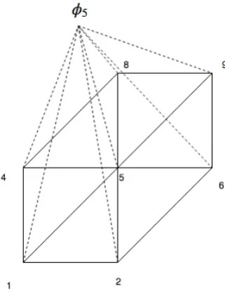
4.2.2 The construction of a Finite element space . . . 33
4.2.3 Error estimate for finite element method . . . 38
4.3 Discretisation of thin plate spline . . . 39
4.4 Lagrangian multiplier . . . 40
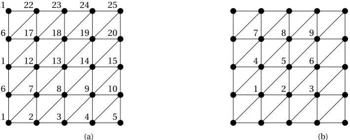
4.5 The Python implementation of finite element discretisation . . . 42
4.5.1 Node-edge data structure . . . 42
5 Multigrid Methods 47
5.1 Poisson’s equation . . . 47
5.2 The classical iterative methods . . . 50
5.2.1 Basic methods . . . 50
5.3 Smoothing effect of classical iterations . . . 54
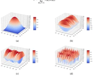
5.3.1 Fourier modes . . . 54
5.3.2 smoothing effect of Jacobi method . . . 56
5.3.3 low, high frequencies and Two-grids . . . 57
5.4 Grid correction . . . 58
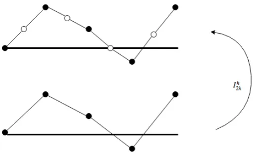
5.4.1 transfer between Two grids . . . 59
5.5 The multigrid V-cycle . . . 62
6 Multigrid Method Solving TPSFEM 65 6.1 Block Smoothers . . . 65
6.1.1 Block Jacobi Method . . . 65
6.1.2 Block Gauss-Seidel Method . . . 66
6.1.3 Block Richardson’s method . . . 68
6.2 Stencil: reduce the computation . . . 68
7 Tests and Error analysis 71 7.1 Two type of errors . . . 71
7.2 convergence behaviour of finite element . . . 72
7.3 Convergence behaviour of Multigrid methods . . . 74
7.3.1 Pure algebraic error tests . . . 75
7.3.2 Test problem 2 . . . 76
7.4 Richardson’s smoother . . . 79
7.4.1 Error convergence of multigrid method with Richardson smoother . . . 81
7.4.2 analysis of multigrid methods with Richardson smoother . . . 82
7.5 Conclusion and Outlook . . . 85
8 Appendix I 87 8.1 Lmatrix on finite element discretisation . . . 87
8.2 G1andG2matrices on finite element discretisation . . . 89
8.3 Amatrix on finite element discretisation . . . 91
9 Appendix II 93 9.1 Topological Space . . . 93
9.2 Poincaré’s inequality . . . 93
C
HAPTER1
Introduction
Functions are the basic mathematical tools for describing many real-life processes. While in some cases functions are known in a explicit formula, very often we come across the problem to construct approxi-mations based on limited information. Such approximation problems are a centre of computational and numerical mathematics.
There are two major types of approximation problems. The first type consists of problems requires to construct approximation based on finite amount of data. As the data often comes from measurement, it is often subject to error and corruption, therefore, uniqueness is often not guaranteed. This type is called interpolation problem. The second types of approximation problems arises from mathematical models. These models often require the determination of unknown functions satisfying operator equations. A simple example of this is using finite element methods to approximate elliptic operator such as the Laplacian.
Our topic Thin plate spline is the first type of approximating problem which is very popular due to its favourable properties. The two dimension the problem is described as a functionu(x) minimises the functional:
Jα(u)= 1 n
n X i=1
³
u(x(i))−y(i)´2+λ
Z
Ω X
|α|=2 2
α!
¡
Dαu(x)¢2
dx
which provides a smoother that predicts response data valuesny(1),· · ·,y(n)o, givenx(i)∈R2is thei-th predictor variable for (1≤i≤n). The functional has two terms: the interpolation term and the smoothing term controlled by smoothing penaltyλthat provides a desired level of smoothness in the approximation at cost of a better fit. The 2nd order derivative is measured in the functional because our humans can’t pickup discontinuities in 3rd degree and higher derivatives, therefore it is good enough for practical use, car surface approximation in safety test as an example. Fun fact: The local approximations of thin plate spline were firstly mentioned by two non-mathematicians but aircraft engineers Harder and Desmarais in[HD71].
plate spline, such a fundamental solution is the radial basis functions, then the solution can be expressed into weighted linear combination of radial basis functions. However, as the radial basis are global, it rises a very poor conditioned linear system. Hegland, Roberts and Altas [RHA03][HRA97][HRA98] later proposed a finite element approximation of thin plate spline (TPSFEM) inR2based on the technique of mixed finite element methods that combines the favorable properties of finite element approximation with those of thin plate splines. This method results in a sparse matrix and the size does not depends on data, the downside is for smallλand large grid size, the matrix is extremely ill-conditioned and also is a saddle point problem. Stals and Roberts in [Sta14][SR06] used preconditioned conjugate gradient to solve the system.
Our motivation is mutual. On the one hand, we want to solve the TPSFEM matrix effectively especially for large grid size with smallλ, it comes from experience of using Multigrid methods efficiently solving Laplacian, which also plays a important role in the matrix of TPSFEM. One the second hand, we want to test Multigrid methods on saddle point problem. We know the Multigrid solver is good at solving elliptic system by removing high frequency component of errors, we wonder if it would still succeed solving this extreme ill-conditioned saddle point problem by exploring its feature. This would be the goal through our study.
The rest of thesis is organised as follows:
Chapter 2 is the preliminary providing an overview of mathematical tools. It has two parts, one part is served for explaining our numerical methods and tests, this parts consists of relatively light mathemat-ical concepts such as basic introduction such as integer order Sobolev space. The other part collects the essential concepts and tools to introduce Duchon’s work as stated in Chapter 3, and we will briefly introduce the concepts of distribution, fractional order Sobolev space, homogeneous Sobolev space and semi-Hilbert space with Hilbert nullspace, based on those knowledge we will be able to introduce the core space developed by Duchon. The definition of Hilbert space, Banach space and quotient space can be found in appendix.
Chapter 3 should be regarded as an extension of this introduction that gives more details about spline the-ory and Duchon’s fundamental work. However, it consists of fairly heavy mathematical contents compared to the rest of the thesis due to the advanced analysis techniques used in [Duc77]. These theories are not so essential for implementing our later numerical work. So we only aim to provide readers a bigger picture of optimal interpolation problem beyond 2-dimensional thin plate splines.
Chapter 4 starts introducing the finite element discretisation of thin plate splines proposed in [RHA03]. We repeat theH1methods that transfers the thin plate splines problem from first type interpolation problem to the second type operator problem to satisfy a variational formula. Then we work on details of finite element discretisation of this variational equation, which allows us to rewrite the thin plate splines problem into linear combinations of basis functions inH1(Ω). We obtain the TPSFEM matrix by applying Lagrangian multiplier. A brief discussion of the programming data structure to construct finite element grid is served for readers interested in implementation.
Chapter 6 consists of our original idea of applying multigrid methods on grid of finite element discretisation to solve the TPSFEM matrix. To simplify the computation, certain assumptions were made to use stencil structures.
Chapter 7 presents the results of numerical tests based on our methods, we firstly verify the convergence behaviour of finite element discrimination by noticingO(h2) convergence rate. Then we have model problems on testing multigrid methods. The results show that multigrid solver using Gauss-Seidel and Jacobi smoothers do not solve for smallλ, but using Richardson’s method as smoother with a careful choice of relaxation parameter, it solves forλ=1e−9. Based on these results, we can verify the efficiency of multigrid solver on our TPSFEM problem. This achieves the goal.
NOTE
C
HAPTER2
Preliminaries
In this chapter we provide a brief summary about the mathematical tools that are used in our work. As we mentioned in introduction, Chapter 3 consists of fairly heavy mathematical contents compared to the rest of the thesis. Therefore we shall separate this chapter into two parts. The first part comes towards the chapters following Chapter 3, where we main introduce the Sobolev space.
2.1
P
ART ONE
: T
OWARDS TO
C
HAPTERS AFTER
C
HAPTER THREE
In chapter 3 we will walk through the optimal interpolation in semi-Hilbert space, from the very general semi-Hilbert space induced by smei-norms on Sobolev space to main problem thin plate spline. We aim to bring up at least the essential ideas in Duchon’s paper, to this end, we will also talk about Hilbert Kernel theory.
2.1.1
S
OBOLEV SPACEThe Sobolev space plays a very important role through our work from two aspects: (1) it measures the fitness and smoothness of interpolation. (2) it provides a good mathematical structure to analyse and approximate solutions. Firstly we define the weak partial derivative,
Definition 2.1. (Weak partial derivative)[Eva98][Definition 5.2.1] Suppose u,v∈L1loc(Ω)(locally Lebegues integrable) andαis a multiidex whereα=(α1,· · ·,αn),αj is a non-negative natural number and|α| =
α1+ · · · +αn. We say that v is theαth-weak partial derivative of u, written
Dαu=v,
provided
Z
ΩuD
αφd x=(−1)|α|Z
Ωvφd x
for all test functionsφ∈Cc∞(Ω), Cc∞(Ω)denote the space of infinitely differentialble functionsφ:Ω→R, compact support inΩ.
Definition 2.2. (Sobolev space)[Eva98][Definition 5.2.2] The Sobolev space
Wk,p(Ω)
consists of all locally summable functions u:Ω→Rsuch that for each multiindexαwith|α| ≤k, Dαu exists in the weak sense and belongs to Lp(Ω).
Remark 2.1. If p=2, we usually denote
Hk(Ω)=W(k,2)(Ω), (k=0, 1,· · ·)
Definition 2.3. (Sobolev norm)[Eva98][Definition 5.2.2] If u∈Wk,p(Ω), for1≤p< ∞, we define its norm to be
kukWk,p:=
X
|α|≤k Z
Ω ¯ ¯Dαu
¯ ¯ p d x 1 p
, (1≤p< ∞)
Note that the Sobolev space consists of functions with smoothness less ?? Therefore, it’s in between ?? Also Sobolev spaces have a good mathematical structure:
Theorem 2.1. [Eva98][Theorem 2 Chapter 5] For each k=1,· · ·and1≤p≤ ∞, the Sobolev space Wk,p(Ω) is a Banach space. Moreover, for p=2, Hk(Ω)is a Hilbert space.
Proof. See
One may also define thefractional Sobolev space, We start by fixing the fractional exponents∈(0, 1): Definition 2.4. (fractional Sobolev space) [NPV11][Section 2]For0<s<1and1≤p< ∞, we define
Ws,p(Ω)=
u∈Lp(Ω) :
¯
¯u(x)−u(y) ¯ ¯ ¯
¯x−y ¯ ¯
n p+s ∈
Lp(Ω×Ω)
i.e. an intermediary Banach space between Lp(Ω)and W1,p(Ω), equipped with the natural norm
kukWs,p(Ω):=
Z
Ω|u| pd x
+ Z Ω Z Ω ¯
¯u(x)−u(y) ¯ ¯ p ¯
¯x−y ¯ ¯
n+sp d xd y
1
p
whens>1 and it is not a integer, we then writes=m+δwheremis an integer andδ∈(0, 1). In this case, the spaceWs,p(Ω) consists of those functionsu∈Ws,p(Ω) whose weak derivativesDαuwithα=|m|, belonging toWδ,p(Ω), namely,
Ws,p:=nu∈Wm,p(Ω) :Dαu∈Wδ,p(Ω),|α| =mo
Definition 2.5. (Fourier transform)[NPV11][Section 2] The Fourier transform onRntakes Lebegue integral function onRnand maps them to functions onRn, defined by
Ff(ξ)= 1 (2π)n2
Z
Rne
−i x·ξf(x)d x (2.1.1)
Definition 2.6. (Fractional Sobolev Space via Fourier transform)[NPV11][Section 2] Now an alternate def-inition of the space Hs(Rn)=Ws,2(Rn)can be precisely defined as
˜ Hs(Rn)=
½
u∈L2(Rn) :
Z
Rn
³
1+¯ ¯ξ
¯ ¯
2s´ ¯ ¯Fu(ξ)
¯ ¯
2
dξ< +∞
¾
note for the above definition, unlike the ones in Gagliardo norm, is valid also for real s>1. With the norm defined by
kukH˜s(Rn):=
µZ
Rn
³
1+¯¯ξ ¯ ¯
2s´¯ ¯Fu(ξ)
¯ ¯
2 dξ
¶12
The fractional Sobolev Space
2.2
P
ART TWO
: T
OWARDS TO
C
HAPTER THREE
In chapter 3 we will walk through the optimal interpolation in semi-Hilbert space, from the very general semi-Hilbert space induced by smei-norms on Sobolev space to main problem thin plate spline. We aim to bring up the essential ideas in Duchon’s paper, to this end, we will also now introduce the Semi-Hilbert space.
2.2.1
S
EMI-H
ILBERTS
PACEDefinition 2.7. (Semi-inner norm[Duc77] LetN be a Hilbert subspace in vector spaceX. A symmetric bilinear form B[u,v] :X×X →Ris called a semi-inner product and the induced nonnegative-valued function p(u)=pB[u,u]is called a semi-norm, if p satisfying the following property:
p(u+v)≤p(u)+p(v),∀u,v∈X p(av)=|a|p(v),∀v∈X,a∈R p(u)≥0,∀u∈X
p(u)=0⇐⇒ u∈N
Notation 1. LetM be a subset of a topological vector spaceY. The orthogonal ofM is defined as
M⊥=©
y0∈Y0| 〈y,y0〉 =0,y∈Mª
The orthogonalM⊥is a linear subspace ofY0.
For a subsetV of the dualY0, its orthogonal inY is defined as
V◦=©
Now we introduce the semi-Hilbert space
Definition 2.8. (semi-Hlbert space with null space)[Duc77] A subspaceX ofE is called a semi-Hilbert subspace with nullspaceN ifXis equipped with an inner product which defines a semi-norm onX with nullspaceN, closed inE, such thatX\N equipped with the quotient norm°°x+N
°
°= kxkis a Hilbert
subspace ofE\N.
Definition 2.9. (reproducing kernel)[Duc77] A linear mappingΦ:N⊥→Eis a reproducing kernel ofX inEif and only if(u0,Φe0)= 〈e0,u0〉for e0∈N⊥and all u0∈X.
The motivation to define the semi-Hilbert space with nullspace and the reproducing kernel for semi-Hilbert space will be explained further with examples in Chapter 3.
2.2.2
H
OMOGENOUSS
OBOLEV SPACES[Wer03] In our later discussion about Duchon’s result in section ??? We need to introduce theHomogenous Sobolev Spaces, also calledBeppo Levi space. For Sobolev spaces we consider all derivatives up to a prescribed order and enssures that the derivatives are Lebesgue-integrable functions. Now if we only consider derivatives of a fixed orderm, then we end up with a semi-normed space. As this is the function space of distributions, we need to introduce the definition of distributions.
Definition 2.10. (Distribution)[Vas10][Definition 5.4] A distribution u ∈D0 is a linear functional on Ccomp∞ (Rn), that is continuous in the sense that u(ϕn)→u(ϕ)wheneverϕn→ϕin Ccomp∞ (Rn).
To understand the above definition, we need to answer what does the convergence mean, i.e. what’s the topology of the spaceD0. The spaceD0is endowed with the weak topology. Precisely inD0, a sequenceTn converges toTin the distribution sense if and only if〈Tn,φ〉 → 〈T,φ〉for allφ∈Dwhere〈·,·〉:D0×D→Ris the duality pair. One should also note that by the defiition, an element inD0(Ω) is uniquely determined by its action onφ∈D(Ω). The action could be very general and abstract as long as it is linear and continuous. Definition 2.11. (homogenous Sobolev space)[?][3.3.6] A homogenous Sobolev space denoted byBm,pfor positive integer m,p after Beppo Levi is the space of all distributions whose derivatives of order m are in Lp, i.e.
Bm,p=©
u∈D0(Rn) :Dαu∈Lp,|α| =mª
with the natural (semi)-norm
|u|m,p=
X
|α|=m m!
α!
° °Dαu
° ° p Lp
1
p
Forp=2 Fourier transform is isometric (Plancherel theorem), the semi-norm can be written as
|u|m,2=
X
|α=m| m!
α!
Z
Rn
¯
¯FDαu(ξ) ¯ ¯
2 dξ
Duchon also showed thatBm,2=Wm,2, therefore we can use the Fractional Sobolev via fourier transform to charaterise
|u|m,2=
X
|α=m| m!
α!
Z
Rn
¯
¯FDαu(ξ) ¯ ¯ 2 dξ 1 2 = µZ Rn ¯ ¯ξ ¯ ¯
2m¯ ¯Fu(ξ)
¯ ¯
2 dξ
¶12
One can see that the motivation of the coefficientsmα!!is from
¯ ¯ξ ¯ ¯ 2m = X
|α|=m m!
α!ξ 2α
The Fourier transform allows us to introduce fractional orders>0 and define
Bs=
u∈D0(Rn) :
µZ Rn ¯ ¯ξ ¯ ¯
2s¯ ¯Fu(ξ)
¯ ¯
2 dξ
¶12
< +∞ , with semi-norm
|u|s,2=
µZ Rn ¯ ¯ξ ¯ ¯
2s¯ ¯Fu(ξ)
¯ ¯
2 dξ
¶12
Now we should be able to introduce the key space in Duchon Definition 2.12. (Semi-Hilber spacesD−mBs) We put
D−mBs:=©
u∈D0(Rn) : Dαu∈Bs,∀|α| =mª
with semi-norm
|u|m,s= µZ Rn ¯ ¯ξ ¯ ¯
2s¯
¯FDmu(ξ) ¯ ¯
2 dξ
¶12
and this space has nullspacePm−1
One may be scared by the spaces defined above, it actually can be seen thatD−mBs(Rn)
=Hm+s(Rn) and Bs(Rn)=Hs(Rn) for−n2<s<n2
Remark 2.2. The main advantage of homogeneous semi-norm is based on the fact that it is invariant through translation and rotation, and also dilations turn into isometry up to a scalar. Those invariance properties are taken into account by Duchon for spline minimisation.
Originally, Duchon considered this space in order to apply for general interpolation problems, he consid-ered a weighting functionωand minimisesR
Rnω2
¯
¯FDmf(ξ) ¯ ¯
2
dξ. He showed fors<n/2,w(ξ)=¯¯ξ ¯ ¯
C
HAPTER3
The traditional approach
The polynomial splines can be introduced from different perspectives, they can be defined as piecewise polynomials with global smoothness properties, or they can be regraded as solutions of an optimisation problem with interpolation as constraints, or they can be linear combinations of certain basis splines. Through this thesis, we shall bring a picture to readers of how these three perspectives relate to each other and play different roles in different uses.
In this chapter, we aim to give a brief survey to the spline problem as an extension of the introduction in Chapter. Starting from the elementary point of view, we give a definition of polynomial splines with a few examples to reveal the first perspective. From that point, we will extend the subject to fit in a general framework of optimal interpolation. This helps us to see the second perspective. Then the concepts of semi-Hilbert kernel and semi-Hilbert space are used to characterise of the problem. These techniques have been originally studied by Duchon. While the work done by Duchon is a general minimisation problem for semi-norm, our core problem rises from a specific case, namely, thin plate spline.
3.1
W
HAT IS SPLINE
: A
BRIEF HISTORY
The idea of spline came from approximating a function or in particular, interpolating between a set of data points. It’s believed that the first mathematical reference to splines is the the 1946 paper by Schoenberg in [Sch46], which is probably the first place the terminology ’spline’ is used to describe functions approximating with piecewise smooth polynomials. In later years , splines have been subject of extensive studies in approximation theory. It was not until 60s, the functional analysis aspect of spline theory evolved and the Hilbert spaces, existence , uniqueness and characterisation theorems where obtained by P.J. Laurent[NS00], M. Atteia [Att92]. However, the lack of constructive and stable methods in many of these concepts made it technically difficult to study concrete examples. They were overcome until Duchon[Duc77] found the representation based on Hilbert kernel theory. This fundamental work has huge impact on the approximating spline functions with radial basis functions. In 90s, a lot of effort were put into numerically approximation splines. [DB02] [Nur89] [SS91].
3.1.1
I
NTERPOLATING SPLINEknots. A example of interpolating spline is showed in fig. 3.1.1
Figure 3.1.1: Interpolating points with polynomials inC1
The plot shows that if a piecewise quadratic approximation that is constructed to pass through a given set ofn+1 points or knots
(x0,z0),· · ·, (xn,zn).
and is quadratic in each of theninterval between them, the global smoothest curve that one can get is theC1smooth given by using quadratic interpolation between each consecutive pair of points. Follow Schoenberg’s definition in Cardinal Spline Interpolation [?], we define
Definition 3.1. (Polynomial Spline) Let n be an integer, n≥0. The symbol
sn={S(x)}
denotes the class of functions S(x)satisfying the following two conditions
S(X)∈Cn−1,
S(x)∈πn in each interval(i,i+1),i=0,±1,±2,· · ·
whereπnstands for the class of polynomials of degree not exceeding n, over the fieldRof real numbers. We call S(x)the polynomial splines of order n−1with knots at the points x1,· · ·,xk.
We shall see that polynomial splines posses the following attractive features:
1. Polynomial spline spaces are finite dimensional linear spaces with simple basis
2. Polynomial splines are relatively smooth functions, and avoids the oscillatory behaviour of polyno-mial interpolations
A simple example of the polynomial spline is the cubic splines:
Definition 3.2. (cubic spline) A function s∈C2is called a cubic spline if s is a cubic polynomial siin each interval[xi,xi+1]. It is called a cubic interpolating spline if imposed with the condition
si(xi)=zi,si(xi+1)=zi+1, 0≤i<n.
the definition does not uniquely define a spline function unless more conditions met. One special kind of cubic spline is callnatural splinecharacterised by their zero second derivative boundary conditions, that is,
s0(x0)=s00(xn)=0. Another example is B-spline standing for Basis spline.
The following result on the existence and uniqueness of splines is stated in [Nur89]: Theorem 3.1.For each i∈©
−m,· · ·,kª
, there exists a unique spline Bimof degree m with knots x−m,· · ·,xk+m+1 such that
Bim(t)=0, t∈(−∞,xi]∪[xi+m+1,∞),
Bim(t)>0, t∈(xi,xi+m+1),
Z xi+m+1 xi
Bim(t)d t=1.
Definition 3.3. (B-spline) The spline Bimin Theorem 2.1 is called the B-spline od degree m with support [xi,xi+m+1]
We mentioned about in [MN90], the work of Polyharmonic spline carried out by Madych and Nelson was partly inspired the ’B-spline’, where they were attempting to obtain a basis for global interpolations. And this follows the idea of interpolating in terms of linear combination of Green’s functions that we will introduce later in Section 3.2.3.
3.1.2
S
MOOTHING SPLINEThe interpolating spline provides a useful way of approximating a smooth functionf(x)∈Cmonly when the data points lie along the path of the function or very closed to it. If the data is scattered at random in the vicinity of the path, then an interpolating polynomial spline, which is bound to follow the same random fluctuations, will belie the nature of the underlying function but oscillate in between the noises. Therefore, the smoothing spliness(x) may be viewed as generalisations of interpolation splines obtained from a set of observationsyi of the targetf(xi). In order to balance the fitness ofs(xi) toyiwith a derivative based measure of the smoothness ofs(x), a penalty parameter may be introduced. The most popular example is the cubic smoothing spline, which is the cubic spline introduced in Definition 3.2 trading off with the smoothness
Definition 3.4. (Cubic Smoothing Spline)
n X i=1
(f(x(i))−z(i))2+λ
Z
D2f(x)d x.
The parameterλis a smoothing parameter, controlling the trade-off between fitness of data and smooth-ness of the function estimate. Asλ→0, meaning there is no smoothing, the estimate spline converges to the interpolating spline. At the other extreme, whereλ→ ∞, the smoothness penalty becomes paramount and the estimate converges to a linear least square estimate.
In this problem the minimiser is known as natural cubic spline mentioned in Definition 3.2 with knots at each sample pointsx1,· · ·,xn.
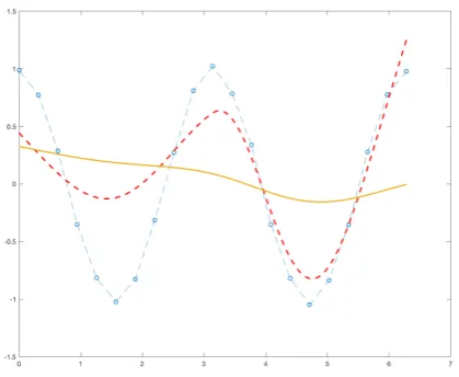
[image:22.595.211.421.339.511.2]In order to have a intuitive understanding of the smoothing spline, Section 3.1.2 shows the cubic inter-polating spline and cubic smoothing spline. One can see that the cubic interinter-polating spline in blue is at least smooth at joint nodes; whereas the cubic smoothing spline with large smoothing parameter in yellow is at most smoother and closes linear regression and the cubic smoothing spline with small smoothing parameter in red has intermediate level of interpolation and smoothness.
3.2
INVARIANT
S
URFACE SPLINE UNDER SEMI
-
NORM
: U
NDERSTANDING
D
UCHON
’
S WORK
Based on the conceptually understanding of splines, we should be very able to introduce our centre problem, namely, thin plate spline, this is the higher dimensional variation of cubic smoothing splines, in two-dimension, we define:
Problem 3.1. (Thin plate spline) For a fixed response vectorz=
n
z(1),· · ·,z(n)owhere each z(i)∈R, and predictorsnx(1),· · ·,x(n)ofor eachx(i)lie in a domainΩ∈R2with convex bounded boundary. Find a function s∈H2(Ω)that minimises the functional
Jα(s)=1 n
n X i=1
(s(x(i))−z(i))2+α|s|2H2(Ω),
where|·|H2(Ω)is the semi-norm of Sobolev space H2(defined in Definition 2.2):
|u|H2(Ω)=
Z
Ω Ã
∂2u
∂x2
!2
+2
Ã
∂2u
∂x∂y
!2
+
Ã
∂2u
∂y2
!2
d xd y
1 2
.
we want to put the problem into a more general frame so that readers could see the whole picture of the optimal interpolation of splines instead of just seeing one specific scope. Readers may see the reduction to get the thin plate spline problem through this approach .
Recall the example we just had for cubic smoothing splines (1-D) and thin plate splines (2-D), the smooth-ness penalty based on the second derivative, and of course this problem can easily be adapted to penalties based on arbitrary derivatives, here we introduce the general case considered by Duchon:
Problem 3.2. (Splines under Sobolev semi-norm) Given an arbitrary set of distinct points©
x1,· · ·,xnª, and for each pointxi∈Rncorresponds to a given value fi∈R. We assume that these fi correspond to function values of a function f from a function space. Find the minimiser u of the problem
minimise |u|m,s (3.2.1)
subject to u(xi)=fi,i=1,· · ·,n. (3.2.2)
where|·|m,sdenotes the semi-norm,
|u|m,s= µ Z Rn ¯ ¯ξ ¯ ¯
2s¯
¯F(Dmu(ξ)) ¯ ¯ 2 dξ ¶1/2 . (3.2.3)
3.2.1
E
XISTENCE AND UNIQUENESSThis section is introduced in the purpose to understand the underlying existence and uniqueness theory of the optimal interpolation under semi-norm in Duchon’s work. As this is not the focus of our work, also we do not want to reinvent the wheel too much, the theorems given in this part will omit the proof. More details may be found in [Duc77], [Att92],
Notation 2. 〈·,·〉denotes the duality pair in the following theorems.
The theory is built in Hilbert kernel theory to semi-Hilbert spaces . LetEbe a locally convex,topological vector space. In our context, we study the caseE is a real vector space. Recall the definition of semi-Hilbert space in Definition 2.8, we now define an interpolant in the semi-Hilbert space by:
Definition 3.5. [Wer03][Proposition 4.4.2](semi-norm interpolation) For a semi-Hilbert subspace ofX⊂E with nullspaceN. LetM be a subspace of the dual spaceE0, we call any element u∗∈X interpolating u0∈X such〈e0,u∗〉 = 〈e0,u0〉for all e0∈Mis a semi-norm interpolation of u0.
In order to show the unique existence of minimal semi-norm interpolation, we need to define another property
Definition 3.6. [Wer03][Definition 5.3.9](unisolvent)For a semi-Hilbert subspace ofX⊂Ewith nullspace
N and semi-Hilbert kernel G, andMa subspace of the dual spaceE0, we callM unisolvent forN if
M◦∩N ={0}.
The terminology unisolvent means uniquely determining an element inN by values in a finite collection ofM.
The following theorem we construct the unique minimal semi-norm interpolation.
Theorem 3.2. [Wer03][Theorem 5.3.12] LetX⊂Ebe semi-Hilbert space with nullspaceN and semi-Hilbert kernelΦ. LetM be a subspace of the dual spaceE0such that the canonical mappingπΦ(M∩N⊥)is closed inX\N. Furthermore, we assumeM is unisolvent forN with positive definiteness i.e.〈e0,Φe0〉 >0for e0∈M∩N⊥\{0}. Then for u0an arbitrary element ofXthere exists a unique pair(e0M,yM)∈M∩N⊥×N such that
uM=GeM0 +yM, is the unique minimal semi-norm interpolation of u0
Proof. The proof can be found in [Wer03].
Theorem 3.2 tells us that optimal interpolation in semi-Hilbert space can be explicit expressed by the basis of the dual space and nullspace. Now we take a example (in an abstract fashion) to see how it works and the readers would also see the connection to our thin plate spline when introduced in later sections. Example 3.1. LetX be a semi-Hilbert space as subspace ofE,©
y1,· · ·,yk ª
be a basis forN, andM =
M◦∩N ={0}.
For u0∈X, let u∗be a minimal semi-norm interpolation of u0forM. By assumption and Theorem 3.2, u∗ is unique and of the form
u∗= n X i=1
biΦe0i+ k X j=1
cjyj,
where the coefficient vectorbandcsatisfy the linear system of equations
〈e0i,Ge0j〉 〈ei0,yk〉
〈e0j,yk〉T 0
b
c
=
〈e0 i,u0〉
0
. (3.2.4)
Remark 3.1. The linear system eq.(3.2.4)guarantees the existence and uniqueness of solution. i.e. the non-singularity of the matrix, however, to see the reason we need to pay more attention on the semi-Hilbert kernel G, namely, G needs to be dense which is ensured by the positive definiteness condition. [Wer03][Theorem 5.3.13]
Use this Hilbert kernel theory, Duchon showed the existence and uniqueness as follows:
3.2.2
O
PTIMAL INTERPOLATION IND
−mB
sThe abstract frame in Duchon’s work [Wer03] had been established in the previous section. Duchon intro-duced the semi-Hilbert spaceX to beD−mBs(Rn) or just simplyD−mBswhich is defined in Definition 2.12 and problem 3.1 .
Note the following proposition gives us the nullspace ofD−mBs Proposition 3.1. The following statements are equivalent
(a) DαP=0,P∈D0, |α| =m
(b) P is a polynomial of order not exceeding m−1.
therefore, equipping with the semi-norm|u|m,s, the nullspace ofD−mBsisPm−1denoting the space of polynomials, whose degrees do not exceedm−1 in anynvariables.
Now we can use these concrete objects to fit in the abstract optimisation theory in last section Theorem 3.2. In [Duc77], they are allocated as follows:
• N :=Pm−1,
• E:=Hl ocm+S: defined in Definition 2.4.
Then the Theorem 3.2 can be read in
Theorem 3.3. [Duc77] LetMbe a closed linear subspace ofE0, such that if p∈Pm−1andMis unisolvent for Pm−1. Then there exists a unique element u∗∈D−mBssatisfying〈e0,u∗〉 = 〈e0,u0〉,∀u0∈M, with minimum semi-norm°°u∗
° °
m,s. LetΦbe a reproducing kernel of D−mBsin Hl ocm+s. Then the u∗has the form
u∗=ΦeM+pM,
for³e0M,pM´∈M∩P⊥m−1×Pm−1.
Proof. The proof can be found in [Duc77].
Theorem 3.3 shows the existence and uniqueness of the solution to problem 3.1. Furthermore, we can see if we let
M=Span©
e1,· · ·,enª, ¡ei∈E0,j=1,· · ·,n ¢
.
Then there exists a unique minimal semi-norm interpolationu∗which is of the form
u∗(x)= n X i=1
λiΦei+ k X j=1
ckpk(x). (3.2.5)
with coefficientsλ=©
λ1,· · ·,λnª.
3.2.3
C
ONSTRUCTIONP
OLYHARMONIC SPLINE One of the result that Duchon proved is thatD−mBs=Hm+sif−m−n2<s<n
2, therefore if we reduce the problem 3.1 by puttings=0, then we have a interpolation problem under the homogeneoussemi-norm |u|mdefined in Definition 2.11, that is,
|u|m= Z
Rd
X
|α|=m m!
α!
¡
Dαu¢2
d x.
Denoting the space to beD−mby takings=0, then we see theD−mis a semi-Hilbert space and we can apply the theory of reproducing kernels. In fact, one of Duchon’s main result is to show that the semi-reproducing kernel ofD−mcan be explicitly found by taking the fundamental solution of polyharmonic operator:
∆ku =0
Definition 3.7. (Green Function)[ACL83]. The form of the Green function of the polyharmonic operator∆m inRnis:
Φm,n(r)
r2m−nlogr, d even
r2m−d, d odd
Once we know the reproducing kernel for the semi-Hilbert spaceD−m, we can construct the minimiser following eq. (3.2.5)
3.3
T
HIN PLATE SPLINE
: W
HAT WE ARE INTERESTED IN
Now we shall make a final reduction, lets=0,m=2 andd=2, then we are in fact interpolating in the Hilbert spaceH2(R2), the interpolation equation is therefore taken up minimising
minimise |u|H2
subject to u(xi)=fi,i=1,· · ·,N where the semi-norm|u|H2(R2)is induced by:
(u,v)H2=
Z
R2
X
|α|=2 2
α!D
αuDαvd x.
This is thethin plate splinein problem 3.1. And applying the Green’s function as reproducing kernel for eq. (3.2.5) directly, we have the unique minimiseru∗in the form
u∗(x)= n X i=1
λi ° °x−xi
° °
2 log°
°x−xi °
°+p(x), p∈P21,x∈R2 (3.3.1)
under Euclidean norm. Further, the coefficientsλiare constrained by the conditions
n X i=1
λip(xi)=0, ∀p∈P21 (3.3.2)
In the traditional approach [Pow93], (3.3.1) and (3.3.2) are together considered to provide a square linear system in the unknowns {λi,i=1,· · ·,n} and {c0,c1,c2}. Write the system in the form
Φ P
PT 0
λ c = f 0 (3.3.3)
HereΦisn×nmatrix and the elements
½ ° ° °xi−xj
° ° ° 2 log ° ° °xi−xj
° °
°:i,j=1,· · ·,n ¾
, andP isn×3 matrix, with i-th row being the vector¡
1 xi yi¢. Further,λcandf are the vectors that have the components ©
that the (n+3)×(n+3) matrix of the system (5.3.3) is nonsingular as long as the dataf doe not lie on a plane, therefore the the spline is uniquely determined.
One of the main issue with this approach is that solving this problem using simple solver will counter with a matrix that is extreme dense. Another issue is that this matrix is not positive definite, ruling out the possibility to use methods like conjugate gradient, but this can be avoided certain matrix computation techniques.
Essentially the difficulty of solving the linear system is due to the saddle-point-problem properties.
3.4
N
UMERICAL SOLUTION
:
THE SADDLE POINT PROBLEM
Recall the words mentioned in the very beginning of this chapter, along the traditional approach, we have transitioned the thin plate spline problem from a optimisation problem to now finding the linear combination of basis. We also briefly mentioned the difficulty of solving such a linear system. Since our goal is to solve thin plate spline numerically, it is worthwhile to classify our numerical subject, which in fact turns out to be a saddle point problem.
The thin plate minimiser solved by eq. (3.3.3) can be extended to the solution of block 2×2 linear system of the form
A PT1
P2 −C
x
y
=
f
g
(3.4.1)
whereA∈Rn×n, P1,P2∈Rm×n, C∈Rm×n, withn≥m (3.4.2) Definition 3.8. saddle point problem[BCL05] If the linear system described above is a saddle point problem, the constituent blocks A,P1,P2and C are satisfies one or more of the following conditions:
1. A is symmetric: A=AT,
2. The symmetric part of A, H≡12(A+AT)is positive semi-definite,
3. P1=P2,
4. C is symmetric and positive semi-definite,
5. C=0(zero matrix).
C
HAPTER4
Finite element discretisation of thin plate spline
We have already seen that the traditional approach leads to a saddle point problem with the linear system involving computation inO(n) in complexity wherenis the number of data, and this is a serious issue, especially for the modern computation that number of observations can be of the order of millions. Besides this, another shortcoming of the system obtained from the reproducing kernel Hilbert space is the fact that such splines do not have a localised basis and a restriction to the case of the finite domain. In order to overcome the those issues, a more capable of large data smoothing method were proposed in [RHA03],[HRA97],[HRA98], which can be viewed as a discrete thin plate spline. In this following section , we can see this method using first order techniques that is tightly relating to the mixed finite element techniques solving the decomposition biharmonic equation[BF91].
4.1
H
1METHOD
Problem 4.1. Recall the thin plate spline in problem 3.1 For a fixed response vectorz=nz(1),· · ·,z(n)o where each z(i)∈R, and predictorsnx(1),· · ·,x(n)ofor eachx(i)lie in a domainΩ∈R2with convex bounded boundary. Find a function s∈H2(Ω)that minimises the functional
Jλ(s)=1 n
n X i=1
(s(x(i))−z(i))2+λ|s|2H2(Ω).
TheH1method transfers the thin plate splines fromH2(Ω) toH1(Ω), the space ˜H1×R3was introduced in [HRA98], where ˜H1(Ω) is the subspace of the Sobolev spaceH1(Ω) consisting of functions with zero mean. The following proposition shows ˜H1is a closed subspace, therefore it endows the same norm.
Proposition 4.1. H˜1(Ω)is a closed subspace of H1(Ω). Proof. let`(u)=R
Ωud x, hence`is a continuous linear functional asΩis bounded. As
`:H1(Ω)3u−→
Z
Ωud x
Consider the following the boundary value problem:
∆s=div(u) inΩ (4.1.1)
∇s·n=u·n on∂Ω (4.1.2)
Z
Ωu=0 (4.1.3)
Leave this boundary value probelm for now. The following functional ˜Jλ(u,c) was considered in [HRA98] for pairs (u,c)∈H˜1×R3
ˆ
Mλ(u,c)=n−1¡
Pu+Xc−y¢T¡
Pu+Xc−y¢
+λ|u|2H1
and the associated bilinear formaand linear formFgiven by
a(u,c;v,d)=n−1¡
Pu+Xc−y¢T¡
Pu+Xc−y¢
+λ
³ ¡
u1,v1)H1
¢
+¡u2,v2
¢´
(4.1.4) F(v,d)=n−1¡
Pv+Xd¢T
y (4.1.5)
where
Pu:=³s(x(1)),· · ·,s(x(n))´T
and
X:=
Ã
1 · · · 1
x1(1) · · · x1(n)
!T
∈Rn,3
The definition of bilinear form will be introduced in later section. At this stage it is sufficient to know the results showed in [HRA98] that ˆMλ(u,c) has a unique minimiser in ˜H1(Ω)×R3if the data points are not collinear. Furthermore, the minimiser can be determined by the problem.
a(u,c;v,d)=F(v,d), ∀(v,d)∈H˜1×R3
Next in vector calculus we have the following theorem that guarantees theuis a gradient of a function. Theorem 4.1. If Ωis a simple connect open set, then for a vector fieldu:Ω→R, there exist a scalar function
φsuch thatu= ∇φif and only if ∇ ×u≡0,i.e.uhas zero curl.
Problem 4.2.
ˆ
Jλ(u)=1 n
n X i=1
(fu(x)−yi)2+λ|u|H1
The converse is also true, precisely we can write
Theorem 4.2. For minimum u∗of Problem 2 is taken over all functions u∈H˜1with zero curl, then there exists s with zero mean such that∇s=u and fu(x)=s(x)+c0∗+c1x+c2y minimises Problem 1 for some coefficientsc.
Proof. We just need to check¯ ¯fu(x)
¯
¯H2(Ω)=|u|H1(Ω)2
Compute the right-hand side
¯ ¯fu(x)
¯ ¯H2(Ω)=
Z
Ω Ã
∂2f
u
∂x2
!2
+2
Ã
∂2f
u
∂y∂x
!2
+
Ã
∂2f
u
∂y2
!2
=
Z
Ω Ã
∂2s
∂x2
!2
+2
Ã
∂2s
∂y∂x
!2
+
Ã
∂2s
∂y2
!2
On the other hand we have, |u|2H1(Ω)2=
¯ ¯u1
¯ ¯
2
H1(Ω)+
¯ ¯u2
¯ ¯
2
H1(Ω)
=
Z
Ω Ã
∂u1
∂x
!2
+
Ã
∂u1
∂y
!2
+
Ã
∂u2
∂x
!2
+
Ã
∂u2
∂y !2 = Z Ω ∂ ∂x à ∂s ∂x ! 2 + ∂ ∂y à ∂s ∂x ! 2 + ∂ ∂x à ∂s ∂y ! 2 + ∂ ∂y à ∂s ∂y ! 2 = Z Ω Ã
∂2s
∂x2
!2
+2
Ã
∂2s
∂y∂x
!2
+
Ã
∂2s
∂y2
!2
=¯¯fu(x) ¯ ¯
H2(Ω)
Note thatsof the elliptic boundary value problem (4.1.1)-(4.1.3) also satisfies
(∇s,∇v)L2(Ω)2=(u,∇v)L2(Ω)2, ∀v∈H˜1(Ω) (4.1.6)
where (u,v)L2(Ω)2=(u1,v1)L2(Ω)+(u2,v2)L2(Ω).
Proof. Multiplying a test functionv∈H1(Ω) on (4.1.3), and by integration by part
Z
Ω∆s·v= Z
Ωdiv(u)·v
−
Z
Ω∇s· ∇v+ Z
Ωv
∂s
∂n = −
Z
Ωu· ∇v+ Z
∂Ω(u·n) Z
Ω∇s· ∇v= Z
therefore, we can determine the solution inH1(Ω) of eq. (4.1.6) by a givenu. Later we will show that eq. (4.1.6) is a weak formula and forssatisfies eq. (4.1.6), we say it is a weak solution. In fact, by interior H2−regularity of elliptic operator, the weak solution s actually hasH2smoothness.
With theH1method, one gets a first order characterisation of the thin-plate spline for a compact domain Ω. While the equivalence requires the zero curl of smoohter in problem 2, we see in [RHA03] the zero curl condition may be dropped completely, that results in a much easier problem to solve numerically by discretasiation of thin plate spline, and also preserves the similar data fitting to the standard thin plate spline. The convergence result had been shown in [RHA03]. In the rest of this chapter, we will focus on using finite element to discretise the thin plate spline over a finite dimensional subspace ofH1(Ω)
4.2
F
INITE ELEMENT DISCRETISATION
In order to obtain discretisation of the problem, We shall now introduce a standard Finite element frame-work. In later chapter we will see it is naturally associated with multigrid method, which is an efficient solver we develop to find the minimiser.
The key ofH1method induces finding functions∈H˜1(Ω) which is a weak solution of
∆s=div(u) inΩ,
∇s·n=u·n on∂Ω,
Z
Ωu=0.
that satisfying the so-called weak formulation
(∇s,∇v)L2(Ω)2=(u,∇v)L2(Ω)2 ∀v∈H˜1(Ω). (4.2.1)
eq. (4.2.1) lays the foundation of discretisation of the function spaces for approximation. This will be the starting point of the numerical computation. However, we first must see that eq. (4.2.1) does indeed define an objective, and ideally defines a unique object. We put the problem in a general framework, introduce the bilinear form, we have see it from early discussion, we formalise it now.
Definition 4.1. [Eva98] A bilinear form, B[·,·], on a linear space V is a mapping b:V×V→Rsuch that each of the maps v→B[v,w]and w→B[v,w]is a linear form on V . It is symmetric if B[v,w]=B[w,v]for all v,w∈V . For instance, an inner product, denoted by(·,·)is a symmetric bilinear form on a linear space V that satisfies
(1) B[v,v]≥0, ∀v∈V
(2) B[v,v]=0⇐⇒ v=0
B[s,v] :=
Z
Ω∇s∇vd x= Z
Ω∇v∇sd x=B[v,s]
and forα,β∈R
B[αs+βv,w]=
Z
Ω(α∇s+β∇v)∇wd x
=α
Z
Ω∇s∇w+β Z
Ω∇v∇wd x
=α(∇u,∇w)+β(∇v,∇w)
=αB[s,w]+βB[v,w] Example 4.2. a¡
u,clv,d¢
and F¡
v,d¢
in page24 define bilinear forms.
Further, we see
Proposition 4.2. The bilinear form B[·,·]in eq.(4.2.1)satisfies the following property
B[s,s]≥0 and
s=0⇐⇒B[s,s]=0 Proof.
(∇s,∇s)L2(Ω)=
Z
Ω(∇s)
2d x ≥0
It is easy to see thatv=0=⇒ B[s,s]=0, we show the converse, sinceR
Ωs=0, then by Poincare’s inequality
(See Appendix II)
kskL2≤k∇skL2=B[s,s]
thereforeB[s,s]=0 implieskskL2=0,s=0.
We may notice that Proposition 4.2 together with the definition of bilinear form are most of the properties defining an inner product. In certain cases, the bilinear form can be shown to satisfy the following properties as well, let’s define
Definition 4.2. [BS02][Definition 2.5.2] A bilinear form B[·,·]on a normal linear space H is said to be
boundedif∃α≤ ∞such that
¯ ¯B[s,w]
¯
¯≤αkskHkwkH, ∀v,w∈H
andcoercive(V-elliptic) on V ⊂H if ∃β>0such that
In the view of the definition above, this shows that the variational problem is naturally expressed in a Hilbert-space setting. The reasoning is as follows, if the coercivity property along with the assumption for B[·,·] to be symmetric bilinear form hold, it follows that it indeed defines an alternate inner product onV asB[s,s]=0 impliess=0. However, it does not immediately follow thatV is a Hilbert space under this inner product. That is, even thoughV is complete under (·,·)H, it may fail to be complete underB[·,·] . It turns out that this cannot happen whenB[·,·] is both bounded and coercive. Indeed, in that case
p
αkvkH≤kskE≤ q
βkvkH (4.2.2)
wherek·kEdenotes the (energy) norm
kskE=B[s,s]
1
2 (4.2.3)
Two norm satisfy (4.2.2) are said to be equivalent. Hence {sn}→sink·kE, so (V,k·kE) is complete. Note that the bilinear form defined in eq. (4.2.1) is bounded and coercive:
Proposition 4.3. Let B[·,·]denote the bilinear form of right-hand side of eq.(4.2.1), then there existsα,β>0 such that
¯ ¯B[s,w]
¯
¯≤αkskH˜1kwkH˜1,
B[s,s]≥βksk2˜ H1.
Proof. Recall Proposition 4.1 that suggests ˜H1(Ω) is a closed subspace of Hilbert spaceH1(Ω). Therefore k·kH1is equipped by ˜H1(Ω). Let’s firstly showB[·,·] is bounded,
¯ ¯B[s,w]
¯ ¯≤
Z
Ω|∇s· ∇w| ≤k∇skL2k∇wkL2 (Holder’s inequality)
≤kskH˜1kskH˜1
In order to show the coercivity, we need to show the inequality
B[s,s]≡
Z
Ω(∇s)
2d x ≥β
µZ
Ωs
2
+|∇s|2d x
(4.2.4)
To prove (4.2.3), it i sufficient to prove that there is constantCsuch that
Z
Ωs
2d x ≤C
Z
Ω ¯ ¯∇(s)
¯ ¯
2
d x, ∀s∈H˜1(Ω)
again by Poincare’s inequality, (4.2.4) holds following withβ=C1+1.
Definition 4.3. If V is a normed linear space, then alinear functional`on V is a real-valued function on V that is linear:
`(αu+βv)=α`(u)+β`(v), ∀u,v∈V, α,β∈R
More precisely, we distinguish between the linear functional spaceV∗(the dual space), of all linear func-tionals onV, and its subspaceV0⊂V∗of continuous linear functionals onV. The following observation characterise functionals inV0.
Proposition 4.4. [BS02][Proposition 1.7.1] A linear functional,`, on a Banach space,B, is continuous if and only if it is bounded, i.e., if there is a finite constant C such that
¯ ¯`(v)
¯
¯≤CkvkB, ∀v∈B
Proof. The proof can be found in most standard functional analysis textbook, reader might reference [Stein P11]. Briefly, one can check if`is continuous at anyuinB, then`must e continuous at everyu∈B. Second,`is continuous atu=0 if and only if there exists a nonnegativeMsuch that
¯ ¯`(u)
¯
¯≤MkukB ∀u∈B
For a continuous linear functional`, on a Banach space,B, the proposition states that the following quantity is always finite:
° °`
° °
B0:= sup 06=v∈B
`(v) kvkB
one can show that this forms a norm onB0, called the dual norm, and the dual spaceB0is complete with respect to it, i.e.,B0is also a Banach space. The dual space of Banach space need not be a mysterious object. We shall see the following example as the key results of Lebesgue integration theory
Example 4.3. The dual space of Lpcan be easily identified, for1≤p< ∞. From Holder’s inequality, any function f ∈Lq(Ω)with the conjugate componentq1+p1=1can be viewed as a bounded linear functional via
Lp(Ω)3v→
Z
Ωv(x)f(x)d x
and that¯ ¯`
¯ ¯≤
° °f
° °
Lq, one can further show(Lp(Ω))0is isomorphic to Lq(Ω)( maybe more details here) Now we should be able to see the characterisation of right-hand side of eq. (4.2.1) in the following proposi-tion
Proof.
`(v) :=(∇v,u)L2(Ω)2=
Z
Ω∇v·u1d x+ Z
Ω∇v·u2d x
≤k∇vkL2
° °u1
° °
L2+k∇vkL2
° °u2
° ° L2
≤kvkH˜1
° °u1
° °
L2+kvkH˜1
° °u2
° ° L2
=³°°u1 ° °L2+
° °u2
° °L2
´
kvkH˜1
therefore`(v)=(∇v,u)L2(Ω)2is a continuous linear functional withM=
° °u1
° °
L2+
° °u2
° ° L2
Thus, given the variational problem eq. (4.2.1), we can show that the Left-hand side is a bounded, coercive symmetry bilinear form and the right-hand side is a bounded linear functional, we then can apply the Riesz representation theorem directly to verify the existence and uniqueness
Theorem 4.3. (Riesz representation theorem) Any continuous linear functional`on a Hilbert space H can be represented uniquely as
`(v)=(u,v)
for some u∈H . Furthermore, we have
° °`
° °
H0=kukH
Proof. The proof is standard in any functional analysis book, here we reference (stein).
Using Riesz Representation Theorem for our variational problem eq. (4.2.1)
(∇v,∇s)L2(Ω)2=(∇v,u)L2(Ω)2 ∀v∈H˜1(Ω) (4.2.5)
we are able to determine a uniques∈H˜1by givenu. One advantage of theH1method is that it puts much less stringent on the approximation of thin plate spline. However, a more important advantage is that the weak form admits powerful numerical techniques, in particular, the Galerkin method.
4.2.1
T
HEG
ALERKIN METHOD FOR A VARIATIONAL PROBLEMThe Galerkin method gives a constructive approach to find an approximation to the weak solution in a finite-dimensional subspace. It may be stated as follows:
Given a finite-dimensional approximating subspaceH˜h1ofH˜h1and`∈H˜0, findsh∈H˜h1such that: