Czech Republic
2SUPA, Department of Physics, University of Strathclyde, Glasgow G4 0NG,
UK
E-mail:[email protected]
New Journal of Physics13(2011) 013015 (14pp) Received 9 August 2010
Published 13 January 2011 Online athttp://www.njp.org/ doi:10.1088/1367-2630/13/1/013015
Abstract. We examine the physical implementation of a discrete time quantum walk with a four-dimensional coin. Our quantum walker is a photon moving repeatedly through a time delay loop, with time being our position space. The quantum coin is implemented using the internal states of the photon: the polarization and two of the orbital angular momentum states. We demonstrate how to implement this physically and what components would be needed. We then illustrate some of the results that could be obtained by performing the experiment.
Contents
1. Introduction 2
2. Experimental setup of four-dimensional (4D) walk 4
2.1. Step operator . . . 4 2.2. Coin operator . . . 7 2.3. Initial state creation . . . 9
3. Computational results 9
3.1. 2D walk . . . 10
4. Conclusions 11
Acknowledgments 13
References 14
3Author to whom any correspondence should be addressed.
1. Introduction
Quantum walks [1] have been studied in great detail ever since it was shown that they are capable of performing algorithms faster than a classical random walk [2]. They have been used in search algorithms [3,4] and recently a link to quantum computation was reported [5,6]. For a review of the basic properties of quantum walks, see [7].
There are two types of quantum walks: the continuous time quantum walk, specified by a Hamiltonian based on the adjacency matrix of a graph that evolves simply by the Schrödinger equation, and the discrete time quantum walk, which introduces an additional Hilbert space called a coin space that is ‘flipped’ at each step and the particle movement depends upon the coin state. We focus on the discrete time case in this paper and briefly mention the main points next.
The discrete time quantum walk evolves in steps, by applying first a coin operator, Cˆ, to the coin space that ‘flips’ the coin and then a step operator, Sˆ, that moves the particle according to the coin state. One such step is given by
|φt+1i = ˆSCˆ|φti, (1)
where|φtiis the state of the particle at stept, in position and coin space, and is of the form
|φit =
X
n,j
αn,j,t|n, ji, (2)
wherenis the particle position, j is the coin state and theαn,j,t are the amplitudes of the states.
The rich dynamics of quantum walks was studied from several aspects with particular attention paid to the influence of the coin operator on the dynamics. One of the most frequently studied cases is a two-dimensional (2D) coin whereCˆ is the Hadamard matrix
ˆ H = √1
2
1 1
1 −1
. (3)
The step operator Sˆ has the form
ˆ
S=X
n,j
|n+ejihn| ⊗ |ji hj|, (4)
whereej is the position shift due to the jth coin state. Typically unbiased walks are considered
theoretically and experimentally, which are defined byP
jej =0.
Coins of more than two dimensions have been studied theoretically [8]–[10]. They can show complex dynamics depending upon the choice of the coin operator, the structure of position space and the initial coin state [11]–[13]. Higher-dimensional coins allow regimes of the walk that are neither diffusive nor ballistic but localized [14]. Such regimes are not accessible from the classical walk and once again emphasize the uniqueness of quantum walks.
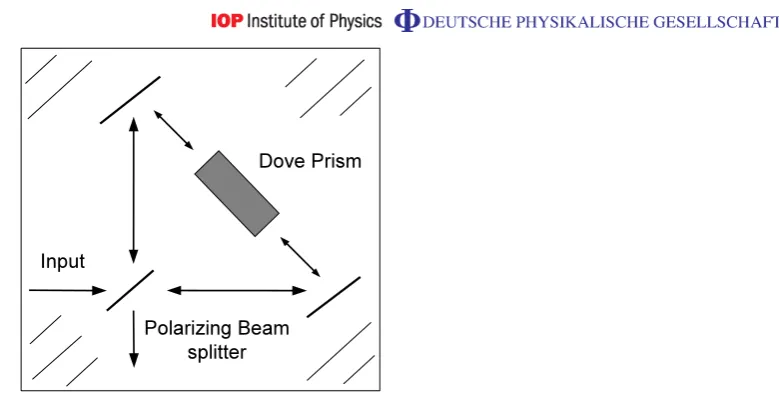
Figure 1. On the left-hand side is the experimental setup used by Schreiber et al [22]. On the right-hand side are the physical realizations of the coin and step operators. In this work, we will replace the half-wave plate and the Mach–Zehnder interferometer with components that act on an extended Hilbert space. The initial state preparation is not shown.
in following sections for our extended coin space. The discussed experiment consists of three parts: preparation of the initial state, the iterative application of the walk operator and finally the detection.
The initial state is produced by attenuating a coherent laser pulse down to the single-photon level, with the average photon number |α|2≈0.1. The effects of multi-photon components
play a role in the measurements only due to detector dead times and thus can be completely eliminated by proper gating. The internal degree of freedom of the walker is represented by the photon polarization. After the walker enters the optical loop its polarization is then rotated to the state |Hi+ i|Vi, which will produce a symmetric distribution in position under the coin used, which is the Hadamard matrix, equation (3). This coin is realized as a half-wave plate (HWP) rotated at 22.5◦. The step operator is a Mach–Zehnder interferometer with polarizing beam splitters (PBS) that send the polarizations along different routes that add different time delays to each polarization. At the end of the loop the walker has a probability to remain in the loop and perform another step or to be out-coupled from the loop to the photodectector. Therefore, this is a probabilistic implementation and the number of steps that the photon undergoes cannot be controlled. By choosing the delay length significantly shorter than the round trip length, the arrival time of photons corresponding to different steps can be easily resolved. The ratio between these two characteristic lengths determines the number of steps one can realize before the intervals corresponding to different steps begin to overlap. The round-trip length can be chosen almost arbitrary at the expense of increased losses in the fibres. The coherence of the system is almost independent of the source since only wave packets that have travelled the same optical paths interfere, and is dominated by decoherence effects within the interferometer. This experiment impressively demonstrates the typical features of quantum walks, such as ballistic spreading and interference, in a very compact setup.
by the appropriate sequence of laser pulses or by using a time-dependent coin. To perform a quantum search a time-dependent coin is needed, which acts on each position state differently.
In this paper, we propose an experimental scheme for a quantum walk with a four-state coin by extending the coin space using the OAM of the photon. This larger coin space will allow us to study more complex dynamics and may open up applications for quantum information processing tasks to be performed. We propose replacements of the physical coin and step operators in figure 1 to operate in this larger space, building upon the ease of this optical implementation.
In section 2, we describe the experimental scheme of the walk, describing the physical implementation of the coin operator, step operator and initial state creation. In section 3, we illustrate some of the results we could achieve from implementing this walk. Section4presents our conclusions.
2. Experimental setup of four-dimensional (4D) walk
In this paper, we propose an implementation of a quantum walk where the quantum coin has four states, which are composed of the polarization and two states of the photon’s OAM. The linear polarizations, horizontal and vertical (H,V), are chosen as the computational basis. The OAM states of our coin space will be Laguerre–Gaussian modes [23], which have an azimuthal angular dependence of eilφ withl= ±1 (we label these +,−). We use these two states because they can be represented on a Poincaré-type sphere on which we can visualize the state transformations in terms of rotations [24]. Our four states are therefore |H,+i,|H,−i,|V,+i,|V,−i. We can relate these to the computational basis |00i,|01i,|10i,|11i and therefore associate the two attributes of the photon (polarization, OAM) with two qubits.
Our physical implementation of the quantum walk consists of three parts: an initial state, a coin operator and the step operator. We describe each in turn below. The physical components of our experiment will be wave plates and PBS for transforming the polarization and mode-converters [25] and Dove prisms for transforming OAM. We combine these to realize the quantum coin operations we need. For example, we can realize a controlled-NOT (CNOT) gate (where polarization is the control qubit and OAM the target) by a Mach–Zehnder interferometer using PBS with a Dove prism in one arm [26]. The step operator displaces our photon throughout position space, which is time here. It can be calculated as the arrival time at the detector and the single position step is specified by the single time delay. All the steps are time delays and so we must change the midpoint of our walk with each step that occurs to obtain the standard quantum walk. In the following subsections, we will describe the mathematical and physical forms of the individual coin and step operators.
2.1. Step operator
Figure 2. SI. This device will be used later and represented as a hashed box in future diagrams.
the coin states by polarization, then to transfer the state from the OAM qubit to the polarization qubit and split the states again with respect to polarization.
In this section, we comment on two possible realizations of the step operator, each with its own advantages and disadvantages. We first describe a component of both step operators, the Sagnac interferometer (SI).
2.1.1. Sagnac interferometer (SI). We wish to spatially separate the four coin states, and although this is easy for the polarization qubit, it is difficult to do this coherently for the OAM state. To solve this problem we aim to transfer the quantum state encoded on the OAM sub-space to the polarization sub-sub-space. To do this we utilize an SI with a Dove prism (rotated at an angleθ) in the path [27], as shown in figure2, with wave plates and mode converters before and after the interferometer. By using an SI and single-qubit polarization and OAM rotating elements, we can achieve the transformation
|Hi ⊗(α|+i+β|−i)→α|H,+i+β|V,−i, (5)
with a similar transformation for the vertically polarized states. The OAM states have become entangled with the polarization and can now be separated at a PBS.
One important point about this transformation is that it will swap the amplitudes of two of the coin states (|H,−i|V,−i). The operation of the SI and wave plates/mode converters on the coin states is
ˆ USI=
1 0 0 0 0 0 0 1 0 0 1 0 0 1 0 0
,
(6)
in the computational basis [|00i|01i|10i|11i]T or using the polarization/OAM basis states [|H+i|H−i|V+i|V−i]T. Our evolution becomes
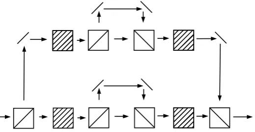
Figure 3. Physical implementation of the step operator. There are four paths here. The hashed box represents an SI and the boxes with diagonal lines represent PBS. The wave plates and mode converters that transform the photon polarization/OAM have been removed for clarity.
Figure 4.Physical implementation of step operator. There are four paths here. The hashed boxes represent SIs and the boxes with diagonal lines represent polarizing beam splitters. The wave plates that transform the photon polarization and OAM have been removed for clarity.
which suggests that we can simply absorb the operation, UˆSI, into our coin operator and also alter our initial state accordingly. Experimentally, this makes the quantum walk more involved to realize, as more qubit gates will be needed to correct the extra operator. This transformation will feature in the next two sections where we describe the step operator in full.
2.1.2. Step operator—version 1. Our first realization of the step operator is shown in figure3. The four coin states enter the step operator where one polarization has a time delay added to it by the first loop. We now entangle the OAM states with polarization, using the SI described in the previous section, and split the polarization again at another PBS. The advantages of this step operator are that it uses the minimum number of components that should reduce the losses and errors in the quantum walk. It has the disadvantage that the time delays added to the coin states are not completely independent of each coin state. This is because the different paths taken by the four coin states are combinations of the two loops and therefore changing the time difference in one loop will alter the time delays added to two of the coin states.
[image:6.595.150.410.250.384.2]state, which we now describe.
By using a device called a ‘q-plate’ [28] we can move our photon from thel= ±1 states into the l=0 state and thus send it through an optical fibre. The q-plate entangles photon polarization and OAM and the transformation for aq-plate with chargeq is
|Li |miOAM|Ri |m+ 2qiOAM. (8)
We first say that we can only use this method in the second version of the step operator, which will become clear soon. We introduce a q-plate with q =1/2 before and after our inner time delay loops in figure4. For this to work, we require a specific state entering ourq-plate,
α|R,+i+β|L,−iq−→-plate(α|Li+β|Ri)⊗ |0iOAM, (9)
because when this state passes through the q-plate it will be contained within the zero OAM subspace. We can now pass this state through an optical fibre. It can be shown that in the first version of the step operator we cannot obtain the correct state for both subspaces of the photon polarization, whereas in the second version we have the flexibility to use different wave plates in each loop. After the state has passed through the optical fibres we use anotherq-plate to reverse the transformation of the firstq-plate, thus obtaining the initial state with the appropriate time delays.
2.2. Coin operator
The coin operator is aU(4)matrix that transforms the coin states into one another. To implement our U(4) coin operator, we use the fact that it can be decomposed into a series of CNOT gates and single-qubit gates [29]–[31]. The single-qubit gates can be physically realized as combinations of wave plates and mode converters, whereas the CNOT gate is a Mach–Zehnder interferometer with a Dove prism in one arm [32].
In this paper we will examine two coins: the Hadamard coin, H4, and the Grover coin,UG, although our scheme is flexible enough to implement any coin. We chose these coins because they have been studied extensively in the literature and, in the latter case, produce markedly different evolutions depending upon the input state. It should be possible to demonstrate these different evolutions in an experiment. The coin operators are given by the following matrices:
H4 = 1
2
1 1 1 1
1 −1 1 −1
1 1 −1 −1
1 −1 −1 1
,
UG = 1
2
−1 1 1 1
1 −1 1 1
1 1 −1 1
1 1 1 −1
.
Due to the swap operation in the first implementation of the step operator we will have to modify our physical implementation of the coin operators. This involves left-multiplying the coin matrices byUˆ−SI1 and implementing that operator in the experiment.
The Hadamard coin, H4, is chosen because it has been studied in the two-coin state and
also because it has the form
H4=H2pol⊗H2OAM, (11)
i.e. it will not entangle the two sub-spaces of the coin states and we can therefore study how initially entangled states evolve. The Hadamard coin can be simply realized as a half-wave plate followed by aπ-mode converter, as shown in the quantum circuit diagram below:
H2
H4
=
H2
where the top line represents the polarization qubit and the bottom line the OAM qubit. When we take into account the action of our step operator on the coin states (the SI, wave plates and mode converters),UˆSI, the modified coin operator becomes
H2 •
H4
=
H2
where H0
4=U− 1
SI H4. This modified gate is realized by a half-wave plate and aπ-mode converter
followed by a Mach–Zehnder interferometer with a Dove prism in one arm.
The Grover coin is chosen as it gives rise to interesting dynamics depending on the input state [12]. It is possible to implement the modified Grover coin (taking into accountUSI) as four single-qubit gates and one CNOT gate, as shown below in a circuit diagram:
U1 • U2
UG
=
V1 V2
The single-qubit gates are
U1= e
−iπ/4
√
2
1 1
−1 1
, U2= e
−iπ/4
2
1 −1
−i −i
,
V1= e
−iπ/4
√
2
i 1
−i 1
, V2= e
−iπ/4
√
2
−i −i
1 −1
,
(12)
−20 −15 −10 −5 0 5 10 15 20 0
0.1
[image:9.595.146.413.90.333.2]n
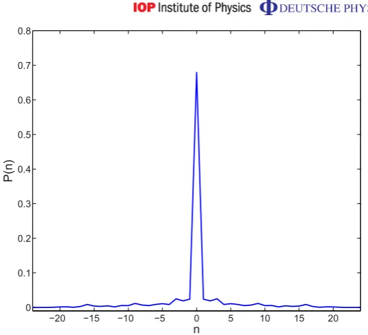
Figure 5.Quantum walk after 12 steps, using the Grover coin and the initial state
|φi1. The probability distribution P(n)is plotted versus positionn. The photon
stays localized around the origin and almost does not spread out in time.
2.3. Initial state creation
We wish to create states of the form
|φi =α1|H,+i+α2|H,−i+α3|V,+i+α4|V,−i (13)
from the initial state|Hi ⊗ |0i, a horizontally polarized photon with zero OAM, assuming that this is the state produced by the laser. We can move this initial state into our coin space by applying a q-plate with q=1/2 [28]. This can then be transformed to a state of the form of equation (13) by using aU(4), as explained in the previous section.
3. Computational results
In this section, we discuss the computational results of our quantum walk. The step sizes used in a quantum walk are usually ±1 but in our walk setup that uses time delays our steps are negative, although we keep the same size difference between steps. We re-adjust the midpoint of the walk at each time step so that the origin falls in the middle of the axis and we obtain the standardized quantum walk. In each figure we sum over all coin states and plot the probability distribution that the state is found at that position versus position. We use the coins mentioned in the previous section and we evolve our walk for 12 steps as this is an experimentally realizable number.
In figures5and6, we use the Grover coin,UGfrom equation (10), with two different initial states,
|φi1= 1
2[|H,+i+|H,−i − |V,+i − |V,−i], (14)
−20 −15 −10 −5 0 5 10 15 20 −0.01
0 0.02 0.04 0.06 0.08
n
[image:10.595.148.410.87.325.2]P(n)
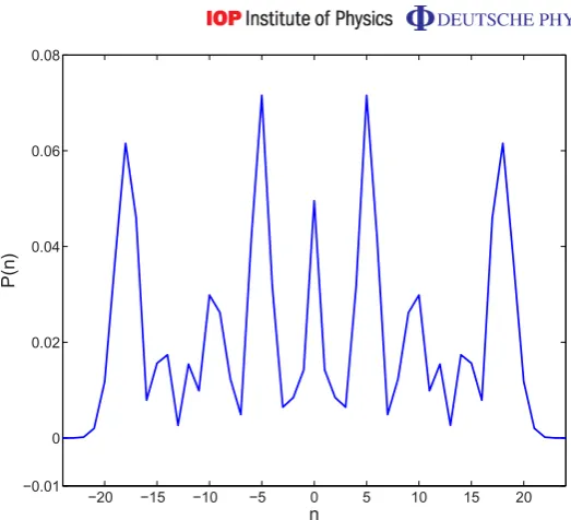
Figure 6.Quantum walk after 12 steps, using the Grover coin and the initial state
|φi2. A marked difference can be seen when compared to figure5with a broad
distribution spread across many position states.
and we can see very different behaviour in the evolution of the state. In figure 5, we can see localization of the wave function about the midpoint and the marked difference compared to figure 6, which shows ballistic spreading over time. This difference is due solely to the initial state used in the device and should be experimentally demonstrable within our scheme. The reason for this is the spectrum of the operatorUG[14].
In figure7, we plot the evolution of the Hadamard coin for 12 steps with the initial state,
|φi3= 1
2[|H,+i+|H,−i+ i|V,+i+ i|V,−i], (16)
which will give a symmetric walk about the origin.
3.1. 2D walk
−20 −15 −10 −5 0 5 10 15 20 0
[image:11.595.148.411.93.329.2]n
Figure 7.Quantum walk after 12 steps, using the Hadamard coin and the initial state|φi3. This distribution is broad comparable to that of figure5.
Figure 8.2D quantum walk after two steps. There is a single point not occupied between the two sections of the walk and we can divide thex-axis into sections labelledy= −2,−1, . . . ,2 (in this case).
4. Conclusions
In this paper, we have proposed an experimental realization of quantum walk using a 4D coin. Our coin space uses the OAM of the photon, the first such proposal. The setup of the quantum walk builds upon a simple implementation already in use that has produced notable results for a large number of steps. We described the physical implementation of coin and step operators and pointed out some of the issues with this realization. Our scheme shows similar advantages as the original scheme in [22], although additional care has to be taken that for the state preparation of initial coin states the position space initial state will use the same methods as before.
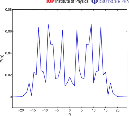
[image:11.595.147.414.384.500.2]−300 −200 −100 0 100 200 300 0
0.01 0.02 0.03 0.04 0.05
n
[image:12.595.150.409.98.323.2]P(n)
Figure 9.2D quantum walk with the Hadamard coin. The probability distribution P(n) versus positionn is plotted. We have a symmetric distribution due to the initial state, which is given by|φi3.
−10
−5 0
5 10
−10 −5 0 5 10 0 0.02 0.04 0.06 0.08 0.1
n
x
n
y
P(n
x
,n y
)
Figure 10.2D quantum walk with the Hadamard coin. By assigning to each point on the time axis a point on an x, y grid, we could build up a 2D picture of the walk.
about the midpoint, whereas the second shows ballistic spreading in time. This difference could be measured easily to verify the basic quantum features of the walk.
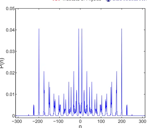
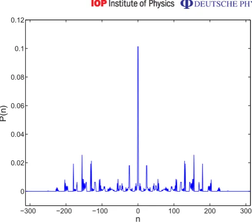
[image:12.595.147.410.404.599.2]−300 −200 −100 0 100 200 300 0
[image:13.595.149.408.92.319.2]n
Figure 11.2D quantum walk with the Grover coin. We have chosen a state that remains localized in time. The initial state is given by|φi1.
−10 −5
0 5
10
−10 −5 0 5 10 0 0.02 0.04 0.06 0.08 0.1 0.12
nx ny
P(n
x
,n y
)
Figure 12. 2D quantum walk with the Grover coin. This is the 2D plot of figure11obtained by giving each point on then-axis a point on anx, ygrid.
Acknowledgments
[image:13.595.147.410.384.564.2]References
[1] Aharonov Y, Davidovich L and Zagury N 1999Phys. Rev.A481687 [2] Farhi E and Gutmann S 1998Phys. Rev.A58915
[3] Shevi N, Kempe J and Whaley B 2003Phys. Rev.A67052307 [4] Gabris A, Kiss T and Jex I 2007Phys. Rev.A76062315 [5] Childs A 2009Phys. Rev. Lett.102180501
[6] Lovett N Bet al2010Phys. Rev.A81042330 [7] Kempe J 2003Contemp. Phys.44307
[8] Mackay T Det al2002J. Phys. A: Math. Gen.352745 [9] Tregenna Bet al2003New J. Phys583
[10] Brun T A, Carteret H A and Ambainis A 2003Phys. Rev.A67052317 [11] Inui N, Konno N and Segawa E 2005Phys. Rev.E72056112
[12] Venegas-Andraca S Eet al2005New J. Phys7221 [13] Liu C and Petulante N 2009Phys. Rev.A79032312
[14] Inui N, Konishi Y and Konno N 2004Phys. Rev.A69052323
[15] Dür W, Raussendorf R, Kendon V and Breigel H-J 2002Phys. Rev.A66052319 [16] Eckert Ket al2005Phys. Rev.A72012327
[17] Xue P, Sanders B C and Leibfriend D 2009Phys. Rev. Lett.103183602 [18] Karski Met al2009Science3251174436
[19] Zähringer Fet al2010Phys. Rev. Lett.104100503 [20] Perets H Bet al2008Phys. Rev. Lett.100170506 [21] Zhang Pet al2010Phys. Rev.A81052322 [22] Schreiber Aet al2010Phys. Rev. Lett.104050502 [23] Allen Let al1992Phys. Rev.A458185
[24] Padgett M J and Courtial J 1999Opt. Lett.24430 [25] Beijersbergen M Wet al1993Opt. Commun.96123
[26] de Oliveira A N, Walborn S P and Monken C H 2005J. Opt. B: Quantum Semiclass. Opt.7288 [27] Nagali Eet al2009Opt. Express1718746
[28] Marrucci L, Manzo C and Paparo D 2006Phys. Rev. Lett.96163905 [29] Vidal G and Dawson C W 2004Phys. Rev.A69010301
[30] Coffey M W, Deiotte R and Semi T 2008Phys. Rev.A77066301 [31] Tucci R R 2005 arXiv:quant-ph/0507171
![Figure 1. On the left-hand side is the experimental setup used by Schreiberet al [22]](https://thumb-us.123doks.com/thumbv2/123dok_us/1683958.121792/3.595.147.466.88.276/figure-left-hand-experimental-setup-used-schreiberet-al.webp)