Stochastic processes induced by Dirichlet (B-) splines: modelling multivariate asset price dynamics

City, University of London Institutional Repository

Citation:

Kaishev, V. K. (2010). Stochastic processes induced by Dirichlet (B-) splines: modelling multivariate asset price dynamics (Actuarial Research Paper No. 195). London, UK: Faculty of Actuarial Science & Insurance, City University London.

This is the unspecified version of the paper.

This version of the publication may differ from the final published

version.

Permanent repository link:

http://openaccess.city.ac.uk/2326/

Link to published version:

Actuarial Research Paper No. 195

Copyright and reuse: City Research Online aims to make research

outputs of City, University of London available to a wider audience.

Copyright and Moral Rights remain with the author(s) and/or copyright

holders. URLs from City Research Online may be freely distributed and

linked to.

Faculty of Actuarial

Science

and

Insurance

Actuarial Research Paper

No. 195

Stochastic processes induced by Dirichlet

(B-) splines: modelling multivariate asset

price dynamics

Vladimir K. Kaishev

June 2010

Cass Business School

106 Bunhill Row

London EC1Y 8TZ

(B-) splines: modelling multivariate asset

price dynamics

by

Vladimir K. Kaishev

Cass Business School, City University, London, UK

Abstract

We consider a new class of processes, called LG processes, defined as linear combinations of independent gamma processes. Their distributional and path-wise properties are explored by following their relation to polynomial and Dirichlet (B-) splines. In particular, it is shown that the density of an LG process can be expressed in terms of Dirichlet (B-) splines, introduced independently by Ignatov and Kaishev (1987, 1988, and 1989) and Karlin et al. (1986). We further show that the well known variance-gamma (VG) process, introduced by Madan and Seneta (1990), and the Bilateral Gamma (BG) process, recently considered by Küchler and Tappe (2008) are special cases of an LG process. Following this LG interpretation, we derive new (alternative) expressions for the VG and BG densities and consider their numerical proper-ties. The LG process has two sets of parameters, the B-spline knots and their multiplicities, and offers further flexibility in controlling the shape of the Levy density, compared to the VG and the BG processes. Such flexibility is often desirable in practice, which makes LG processes interest-ing for financial and insurance applications.

Multivariate LG processes are also introduced and their relation to multivariate Dirichlet and simplex splines is established. Expressions for their joint density, the underlying LG-copula, the characteristic, moment and cumulant generating functions are given. A method for simulating LG sample paths is also proposed, based on the Dirichlet bridge sampling of Gamma processes, due to Kaishev and Dimitrova (2009). A method of moments for estimation of the LG parameters is also developed. Multivariate LG processes are shown to provide a competitive alternative in modelling dependence, compared to the multivariate asymmetric VG process considered by Cont and Tankov (2004) and Luciano and Schoutens (2006), and to its generalization by Luciano and Semeraro (2007) and Semeraro (2008). Application of multivariate LG processes in modelling the joint dynamics of multiple exchange rates is also considered.

1 Introduction

An important strand of literature on financial modelling in recent years is devoted to developing more realistic stochastic models incorporating appropriate Lévy processes as drivers of the price dynamics of financial assets. Examples of such processes are the Variance Gamma process introduced by Madan and Seneta (1990) (see also Madan et al. 1998) and the so called Bilateral Gamma (BG) process considered recently by Küchler and Tappe (2008). The three parameter VG process of Madan et al. (1998) is con-structed by randomly changing the time in a Brownian motion with certain drift and volatility parameters, following a Gamma process with unit mean rate and certain vari-ance rate parameter. The BG process is a generalization of the VG process and its incre-ments have a four parameter Bilateral Gamma distribution, which represents two Gamma distributions, one for the positive and one for the negative half-lines, adjoined together at the origin. Both VG and BG processes are pure jump, infinite activity, finite-variation, Lévy processes, that inherit these properties from the Gamma processes under-lying their construction. For an excellent account on properties of Gamma processes which play an important role throughout this paper, we refer to Yor (2007).

The exponential VG process has proved a successful alternative to Geometric Brownian motion in a number of applications, for example in option pricing (see Kaishev and Dimitrova 2009 and the references therein) and in credit risk modelling (see Schoutens and Cariboni 2009). The ability of the VG process to capture both upward and down-ward jumps as well as very small movements (jitters) in stock prices have been high-lighted by Stein et al. (2007) who give an extensive list of further references on the VG model and its applications.

Many real life financial applications require modelling the joint dynamics of multiple, possibly dependent asset price processes. A typical example would be the necessity to model the joint movement of foreign currencies exchange rates. In such cases, develop-ing models involvdevelop-ing appropriate multivariate Lévy processes, capable of capturdevelop-ing different dependence patterns is of utmost importance. In order to meet such demands, recently, attempts to extend the VG model to more than one dimension have been under-taken in several directions. For example, Luciano and Schoutens (2006) considered a multivariate VG model, in which dependence is achieved by applying a random time change according to a common Gamma process, in the corresponding, differently parame-terized, univariate Brownian motions. The level of dependence in this construction is controlled only through the Gamma variance rate parameter which imposes some limita-tions on its flexibility (see the numerical illustration in Section 4). Further generaliza-tions of this construction, due to Luciano and Semeraro (2007) and Semeraro (2008), allow for a decomposition of the time change in a common and idiosyncratic parts.

In this paper we propose a new class of Lévy processes defined as linear combinations of independent Gamma processes. In what follows, it will be convenient to refer to such linear combinations as LG processes. It is directly verified (see Section 2) that both the Variance Gamma (VG) process and the Bilateral Gamma process are special cases of an LG process represented as particular linear combinations of two Gamma processes.

Our aim in this paper is to introduce univariate and multivariate LG processes, explore their properties and illustrate how they can be applied in modelling the joint behavior of empirical asset price processes. As the VG and the BG, LG processes also preserve some of the nice features of the Gamma processes used for their construction. They are pure jump Lévy processes of finite variation which may jump infinitely many times on a finite time interval. We show that LG processes are intrinsically related to the so called Dirichlet splines and polynomial B-splines, and posses some of their interesting geomet-ric properties. In particular, we give explicit expressions, in terms of multivariate Digeomet-rich- Dirich-let (B-) splines, of the joint density of the LG distribution, generating multivariate LG processes. Dirichlet splines, which have been independently introduced by Karlin et al. (1986) and by Ignatov and Kaishev (1987, 1988, 1989) who call them generalized

B-splines, are densities of linear transformations of Dirichlet random variables. When the

shape parameters of the underlying Gamma processes are integer, the corresponding LG density is expressed in terms of multivariate simplex splines, introduced by De Boor (1976). We give also some new expressions, in terms of univariate Dirichlet (B-) splines, for the densities of the VG and BG distributions. The proposed approach allows for the uniform treatment of the wide class of LG processes in terms of multivariate Dirichlet (B-) splines for which methods of their efficient numerical evaluation exist (see Section 3).

The structure of the paper is as follows. In section 2, we introduce univariate LG pro-cesses, note their relation to the Variance Gamma and Bilateral Gamma propro-cesses, explore their distributional properties and give the Lévy triplet and martingale condi-tions, which characterize them. In section 3, we introduce the multivariate version of an LG process, establish expressions in terms of multivariate Dirichlet (B-) splines for the joint density of its underlying joint LG distribution, give its underlying LG copula, its characteristic, moment and cumulant generating functions. We also provide a method of moments, based on expressing them in terms of cumulants, for estimating the LG parame-ter. In Section 4 we illustrate how the multivariate LG processes are applied in mod-elling the dynamics of the joint movement of the exchange rates of a set of currencies. Section 5 provides conclusions and some further comments.

2 Linear combinations of Gamma (LG-) processes

For the purpose, denote by Git;ai,l, i=0, ..., n a collection of n+1 independent

Gamma processes, defined on a probability space W, , , with mean rate a_il >0

and variance rate ail2>0, where ai>0 and l >0, i=0, ..., n. For a fixed t, t>0, the density of Git;a_i, l is

f_Gix;a_i, l,t= l

ait

Gait

xait-1‰-lx_,

where x>0. Let us recall that the Gamma process, Git;ai,l, is a pure jump, finite

variation process which jumps infinitely many times up to time t and has independent, gamma distributed increments. It plays a central role in contemporary financial mod-elling. For a detailed account on the properties of Gamma processes and their applica-tion in finance and insurance, we refer to Yor (2007), Fu (2007), Dufresne et al. (1991), Dickson and Waters (1993), Madan et al. (1998). We will use the gamma processes,

Git;ai,l, i=0, ...,n, as building blocks and define the process of interest in this paper, as follows

Definition 1. Given a set of real valued distinct parameters d =d0, ..., dn, define the

process LGt;d, a,l, n as a linear combination of the independent gamma processes,

Git;a_i,l, i=0, ...,n, i.e.,

(1)

LGt;d, a, l, n= d0G0t;a0, l+...+ dnGnt;an,l,

where a =a₀, ..., an. For the sake of brevity we call such linear combinations, LG

processes.

In what follows we will sometimes abbreviate LGt;d, a,l, n, to LGt and the two notations will be used interchangeably.

Let us note that the three parameter Variance Gamma process, introduced by Madan et al. (1998), is a special case of an LG process. To see this recall that the VG process,

VGt;q,s, n is defined as

VGt;q,s, n=B G t; 1

n, 1

n ;q,s ,

where Bt;q, s is a Brownian motion with drift q œ and volatility s >0, and

Gt; 1_n, 1_n is a Gamma process with mean rate 1 and variance rate n >0. It is not diffi-cult to see that the VG process admits the alternative, LG representation

(2)

VGt;q,s, n= d0G0t;a0, 1+ d1G1t;a1, 1,

where d0 =

-q2_+2s2_{n -q}

2 n, d1 =

q2_+2s2_{n +q}

2 n; a0= a1= 1

n, which is a special case of

Equality (2) follows from the fact that the characteristic function of the VG process (see Madan et al. 1998), can be expressed as

fVGtu=

1

1-iq nu+ 1

2 s 2_nu2

1

nt

= 1

1+i ud0

a0t ₁

1-i ud1 a1t

=‰i ud0G0t;a0,1+ d1G1t;a1,1_,

where d0 is the absolute value of d0. Furthermore, a linear combination of say, p, VG

processes is also a LG process, i.e.,

VG1t;q0,s1,n1+...+VGp-1t;qp-1, sp-1,np-1=LGt;d, a, 1, 2 p

where d =d0, …, d2p-1, a =a0, …, a2p-1 and dj=

-q2j+2s2jnj-qj

2 nj

j=0, …, p-1, d_j=

q2j-p+2s2j-pnj-p+ qj-p

2 nj-p, j= p, …, 2 p-1 and

aj= ap+j=1nj, j=0, …, p-1.

It can be shown that the Bilateral Gamma (BG) process, recently considered by Küchler and Tappe (2008), is also a special case of an LG process. The BG processes are associ-ated with the bilateral gamma distribution, Ga+, l+,a-,l-, with parameters a+_{, l}+_,a-_,l-_{>0, defined as the convolution}

Ga+_,l+_{, a}-_{, l}-_{:= Ga}+_{, l}+_{* Ga}-_,-l-_,

where Ga,l is a generalized Gamma distribution with parameters a >0, l œ\0. The density of Ga,l is given by

(3)

fBGx;a, l= l

a

Ga x

a-1_‰-l x_

l>0x>0+l<0x<0,

where xœ and _ÿ is the indicator function. As can be seen from (3), when l >0, this is the well-known Gamma distribution, concentrating mass on +, whereas, for l <0,

the generalized Gamma distribution is simply a Gamma distribution on the negative half axis, -. The corresponding bilateral gamma process, BGt;a+,l+, a-,l- is a pure

jump Lévy process, whose increments have bilateral gamma distribution and in particu-lar, for fixed t, t>0,

BGt;a+,l+, a-, l-~Ga+t,l+,a-t, l-.

It is directly verified that, the BG process is a four parameter generalization of the VG process and admits the following representation as an LG process

BGt;a+,l+, a-, l-= d0G0t;a0, 1+ d1G1t;a1, 1,

where d₀ = -1l-; d₁ =1l+ ; a₀ = a-, a₁= a+, l =1 and n=1. As in the case of VG, linear combinations of BG processes are also LG processes, i.e.,

BG₁t;a₀+, l₀+,a-₀,l₀-+...+BGpt;a+_p-1, l+_p-1,a-_p-1, l-_p-1=LGt;d, a, 1, 2 p,

where d =-1l₀-, …, -1l-_p-1, 1l₀+, …, 1l+_p-1 and a =a₀-_{, …, a}

p-1

- _{, a} 0

+_{, …, a}

p-1

+ _.

2.1 Distributional properties

From Definition 1, for fixed t, say t=1, it is directly seen that the characteristic func-tion, f_LGz=‰i zLGt_{, of a LG process is given by}

fLGz=

j=0

n _l

l -id_jz

aj

, zœ.

The cumulant generating function, Yu=ln‰uLGt _{, uœ is}

Yu=

j=0 n

ajln l l - dju

,

where

l maxjœD-dj

<u< l

maxjœD+dj ,

D-= iœI :sgndi= -1, D+=iœI: sgndi= +1,I =1, ..., n.

The cumulants kw= Yw0 , where

Yw_u₌_w-1_! j=0

n

ajdwj l - dju-w, w=1, 2, …

are then obtained as

(4) kw=w-1!

j=0 n _a

j lw dj

w

, w=1, 2, ….

LGt= m_LG= k₁ = 

iœD+ aidi

l -_i_œ D-aidi

l ,

VarLGt= nLG = k2= 

iœD+ aidi2

l2 + 

iœ

D-aidi2 l2

cLG = k3 k232=

j=0 n

2ajd3jl-3  j=0

n

ajd2jl-2

32

tLG=3+ k4 k22 =3+

j=0 n

6ajd4jl-4  j=0

n

ajd2jl-2

2

.

Let us now give an expression for the density of LGt. For the purpose, we will need some notation and background results. Denote by

Sn=x=x1, …, xnœn:xi¥0, for alli,  i=1

n

xi§1,

the standard n-simplex and recall that the random vector q0, ..., qn, has Dirichlet

distribution a0, ...,an on Sn, with (real) parameters a0 >0, ..., an>0, i.e., q0, ..., qnœa0, ...,an, if q0=1- q1-...- qn and the joint probability density of q1, ...,qn with respect to the Lebesgue measure is

f_q1,...,qnx= Ga0+...+ an in=0Gai

 j=0

n

xa_jj-1_xœSn,

where x₀=1-x₁-…-x_n. We will use the shorter notation q₀, ..., qnœ1 if aj=1, j=0, …, n. We will now establish the following property of a LG process, which will be used in the sequel.

Lemma 1. For a fixed t, t>0, the process LGt;d,a,l,n, defined in (1), admits the

representation

(5)

LGt;d,a, l,n= BtGt,

where Gt=n_i=0Git;ai, l, Bt= d0q0+...+ dnqn and the random variables q0, ...,qn, have a Dirichlet distribution a0t, ..., ant with (real) parameters a0t>0,

Proof. Representation (5) follows from the fact that, for fixed t, the r.v.s q₀, ..., q_n, coincide in distribution with the random variables Git;ai, l Gt, i=0, ...,n (see e.g. Wilks 1962), and by the theorem of Sukhatme (1937), the latter are independent of Gt

which yields the independence of Bt and Gt.á

Lemma 1 is fundamental in the study of LG processes since it links their underlying LG distribution to the classical polynomial splines and in general to the so called, general-ized B-splines (known also as Dirichlet splines). This link, as will be demonstrated, provides a different, spline-approximation insight into the distributional properties of LG processes. It is interesting, both from the theoretical and numerical point of view, since the theory of polynomial spline functions is well developed (see e.g. Schumaker 1981) and offers also numerically efficient recurrence formulas for the evaluation of (B-)splines (see De Boor 2001) which, as we will see, can be useful in dealing with LG distributions.

In order to follow the link of the distribution of LGt;d, a, l, n to splines, provided by Lemma 1, let us first note that, for integer values of the parameters a₀t>0, ..., a_nt>0, the density, fBtx, of the random variable, Bt, coincides with a polynomial B-spline. This is an important probabilistic interpretation of B-splines, established independently by Ignatov and Kaishev (1985, 1989) and Karlin et al. (1986). In order to give a more precise formulation of this result, which will be used in the sequel, let us recall some background properties of polynomial B-splines. Let d =d0, ..., dn denote a set of

distinct real values, called knots of the spline and denote by a =a₀, ..., an the set of their corresponding integer-valued multiplicities. The multiplicity ai=1, 2, .., equals the number of repetitions of the knot di in the set of possibly coincident knots of the

spline. Let us recall that the polynomial B-spline M x;d₀,

a0,

...,

...,

dn

an

of order

r= a0+...+ an-1 (degree r-1) with knots d =d0, ...,dn of multiplicities

a =a0, ...,an coincides with a polynomial of degree r-1 between its adjacent

(distinct) knots and is defined as the r-th order divided difference of the function

fy=ry-x₊r-1, i.e.,

M x;d0,

a0,

...,

...,

dn

an

=d0, ..., dn fy.

The B-spline M x;d0, a0,

...,

...,

dn

an

has the following explicit representations. If knots are

pair-wise distinct, i.e., their multiplicities a0=1, ..., an =1, then

M x;d₀,

1,

...,

...,

dn

1

=n

i=0 n

di-x+n-1  

j=0,j∫i n

If some of the knots coincide, i.e., a0 ¥1, ...,an¥1, then

M x;d₀,

a0,

...,

...,

dn

an

=_

i=0 n

Dai-1xidi  a

i-1!,

where xiy=ry-x₊d-1 j₌₀ j∫i

n _

y- djn-1 and Dai-1 _{denotes the} a

i-1-th derivative.

The following theorem, due to Ignatov and Kaishev (1989) establishes an important probabilistic interpretation of polynomial B-splines which we will use to study the distributional properties of LG processes.

Theorem 1. (Ignatov and Kaishev 1989). The polynomial B-spline M x;d0,

a0,

...,

...,

dn

an

of

degree a₀+...+ a_n coincides with the density fBx, with respect to the Lebesgue mea-sure of the random variable

B= d₀q₀+...+ d_nq_n,

where the random variables q₀, ..., q_n have joint Dirichlet distribution with parameters, a0, ..., an, i.e., q0, ..., qnœa0, ...an.

Let us note that the Dirichlet parameters a0, ..., an, may in general take real values. In this case the density, fBx, has been viewed by Ignatov and Kaishev (1987, 1988) as a generalized B-spline. Independently, Karlin et al. (1986) have also considered similar generalization of B-splines. Later, such densities have been named Dirichlet splines (see Neuman 1994 and zu Castell 2002). Here and thereafter, we will use the two terms, generalized B-splines and Dirichlet splines interchangeably. For consistency with the

polynomial B-spline notation, we will alternatively denote, fBx as Mg x;d0, a0,

...,

...,

dn

an

, to

stress its interpretation as a generalized B-spline i.e. a Dirichlet spline. We will make use of the following properties of generalized B-splines.

Denote by d =d₀, ...,dn, the set of distinct knots, d_iœ, and by a =a₀, ...,an the set of (positive real) multiplicities of d =d0, ...,dn. Denote also by a`i, the integer part of ai, and by ai= ai- a`i, its fractional part. Without loss of generality, assume that, ai>0, i=0, …, r and that, and ai=0, i=r+1, …, r+m, n=r+m.

The generalized B-spline can be expressed as the following divided difference (see Ignatov and Kaishev 1988)

Mg x;d0,

a0,

...,

...,

dn

an

=da`00,,

...,

...,

dr,

a`r,

dr+1,

ar+1,

, ..., d_r+m

ar+m

Hu, if xœD

where

Hu= Ga0+...+ ar+m

Gl-1Ga0 ...Gar Sr

u-x+

i=0 r

di-uyi

+

l-2

y₀a0-1

...y_rar-1„_y

0...„yr,

l=_ir₌₀+ma`<sub>i</sub>, (l¥2), S<sub>r</sub>=y<sub>0</sub>, ..., yr: 0§ y<sub>i</sub>, i=0, ..., r, y<sub>0</sub>+...y<sub>r</sub>§1 and D is the set of all d<sub>i</sub>'s for which a`_i¥1, D denotes the convex hull of D.

The numerical evaluation of generalized B-splines is facilitated by their representation in terms of classical polynomial B-splines, due to Kaishev (1991). For further properties of generalized B-splines (i.e. Dirichlet splines) we refer to Neuman (1994) and zu Castell (2002).

We can now formulate and prove the following proposition which expresses the density of LGt in terms of Dirichlet splines.

Proposition 1. For fixed t, the density, f_LGtx, of LGt;d, a,l, n is given by

(6)

fLGtx=

0

+¶ _la0+...+ant

Ga0+...+ ant

ya0+...+ant-2‰-ly_M

g

x

y;ad00t,,

...,

...,

dn

ant

„y,

where Mg x_y; d0, a0t,

...,

...,

dn

ant

, is a Dirichlet spline with knots, d0, ..., dn, of (real)

multiplici-ties, a0t, …, ant.

Proof. By Lemma 1, we have that LGt;d, a,l, n is expressed as a product of two

independent random variables with known densities. More precisely, the random vari-able, Gt=_in₌₀Git;a_i,l, is gamma distributed with parameters a₀+...+ ant and l, i.e., Gt~Gammaa0+...+ ant, l, whereas, by Theorem 1, the density fBtx, of the random variable, Bt, coincides with a generalized B-spline. We will denote the density of Gt, as fGtx.

Thus, we have

fLGtx=

d

d x PBtGt§x

= d

d x PBt§xGt

= d

d x 0

+¶

PBt§xy f_Gty„y

= _

0 +¶

f_Btxy f_Gty 1

y „y.

(7)

fGty=

la0+...+ant

Ga0+...+ ant

ya0+...+ant-1‰-ly_,

and that f_Btxy coincides with a generalized B-spline, M_g xy; d₀,

a0t,

...,

...,

dn

ant

. á

Several properties of the process LGt;d, a,l, n easily follow from Proposition 1.

Corollary 1. If ait are integer valued, the density, fLGtx, of LGt;d,a, l, n is given

by

(8)

fLGtx=

0

+¶ _la0+...+ant

Ga0+...+ ant

ya0+...+ant-2‰-ly_M x y;ad00t,,

...,

...,

dn

ant

„y,

where M x

y;_ad0,

0t,

...,

...,

dn

ant

, is a polynomial B-spline with knots, d0, ..., dn, of

multiplici-ties, a0t, …, ant.

Corollary 2. The density of the increments, LGt+h;d,a, l,n-LGt;d,a,l,n ,

h>0 is given by



0

+¶ _la0+...+anh

Ga0+...+ anh

ya0+...+anh-2‰-ly_M

g

x

y;ad00h,,

...,

...,

dn

anh

„y.

Proof. We have

LGt+h;d,a,l,n-LGt;d, a, l, n=

d0G0t+h;a0,l-G0t;a0, l+...+ dnGnt+h;an,l-Gnt;an,l,

which, for fixed t and h>0, is a linear combination of gamma variates

gi=Git+h;ai, l-Git;ai, l with density

f_gix;ai,l,h=

laih

Gaih

xaih-1‰-lx_.

Obviously, for fixed t and h>0 we can write

LGt+h;d, a,l, n-LGt;d,a, l, n=d0g0+...+ dngn   i=0

n

gi 

i=0 n

gi,

We conclude this section by noting that the following proposition which is a direct consequence of the scaling property of the gamma distribution provides an alternative way of expressing the underlying LG distribution, as a linear combination of n+1 gamma variates with different shape and scale parameters.

Proposition 2. The process LGt;d, a, l, n admits the representation

(9)

LGt;d,a, l,n=sgnd₀G₀t;a₀, l d₀ +...+sgndnGnt;a_n, l d_n .

It has to be noted that extensive literature exists which deals with the distribution underly-ing (11), in the special case when sgndj= +1, j=0, …, n. In the latter case, an

explicit formula for the density of LGt;d, a,l, n when t is fixed, t>0, is given by Moschopoulos (1985).

2.2 The Variance Gamma and the Bilateral Gamma special cases

New expressions for the density of the Variance Gamma, VGt;q,s, n and the Bilat-eral Gamma processes directly follow from their LG representation, Proposition 1 and Corollary 1. We have

Corollary 3. For fixed t, the density, fVGtx;q,s,n, of the Variance Gamma process,

VGt;q,s, n is given by

(10)

fVGtx;q, s,n=

0

+¶ ₁

G2tn y

2tn-2_‰-y

Mg

x

y;

-q2_+2s2_{n - q}

2 n,

tn

q2_+2s2_{n + q}

2 n

tn

„y,

where M_gx

y;tÿn, tÿn coincides with a classical polynomial B-spline of degree

2t

n -2 if

t

n

is integer. Recall that a different expression for the density f_VGtx;q, s, n, has been given by Madan et al. (1998) as follows

fVGtx;q,s, n=

0

+¶ ₁

s 2py

‰-

x-qy2

2s2_y 1 nnt G_tn

ytn-1‰

-y

n „_y.

For the density of the Bilateral Gamma process we have ,

Corollary 4. For fixed, t>0, the density, fBGtx, of the Bilateral Gamma process,

BGt;a+,l+,a-,l-, is given by

(11)

fBGtx=

0

+¶ ₁

Ga-_{+ a}+_t y

a-_+a+_t-2 ‰-y_M

g

x

y;-l

-_-1_, a-_t l

+_-1 a+_t

where Mgx_y;_a-ÿ_t, _a+ÿ_t coincides with a polynomial B-spline of degree a

-_{t+ a}+_{t-2 if}

the parameters, a-t, a+t, are integer. For comparison with (11), for t=1, the density,

f_BGtx given by Küchler and Tappe (2008) is

fBGx= l

+_a+ l-_a -l+_{+ l}-_a+_+a-_2

Ga+_ x

a0+a12-1‰-xl+-l-2_W

a+_-a-_2,a+_+a-_-12xl++ l-,

where W_w,mz is the Whittaker function defined as

Ww,mz=

zw‰-z2

Gm - w +12 0 +¶

tm-w-12‰-t1+ t

z

m+w-12

„t

form - w > -1 2.

In conclusion, let us note that expressions (6), (8) (10) and (11), involving generalized or polynomial B-splines, are numerically appealing, due to the recurrent computation of polynomial splines (see De Boor 1976) and the cubature formula for generalized B-splines (i.e. Dirichlet B-splines) in terms of polynomial B-B-splines, due to Kaishev (1991).

2.3 The Lévy triplet and related properties

As known, (see e.g. Cont and Tankov 2004, Section 3.4), the characteristic triplet, g, A, k, i.e., the Lévy triplet of a (multivariate) Lévy process, comprised by, a (real) vector g, a positive definite (covariance) matrix A and a positive measure k, related to its Itô decomposition, uniquely determines its distribution. Following the Lévy-Khinchin representation formula, it is possible to express the characteristic function, fLGz=‰i zLGt, of a LG process, in terms of its corresponding Lévy tripletg, A,k

and deduce some path-wise properties. The following Proposition gives the Lévy triplet of an LG process.

Proposition 3. LGt;d,a,l,n is a Lévy process with characteristic triplet g, 0, kL G,

where the Lévy measure kL G„x is given by

(12) kL G„x= 

iœ D-ai‰

-l x

di

x x<0+

iœD+ ai‰

-lx

di

x x>0 „x

(13) g = 1

l _i_œD+aidi 1- ‰

-_dl

i -

iœ

D-aidi 1- ‰

-_dl

i < ¶.

Proof. Since LGt;d,a,l,n is defined as a linear combination of the gamma

pro-cesses, Git;a_i, l, i=0, ..., n, which are Lévy processes, LGt;d,a, l,n is also a Lévy process (see, e.g. Theorem 4.1 of Cont and Tankov 2004). Expression (12) for the Lévy measure kL G„x follows from the additivity property of the Lévy measure (see e.g. Proposition 5.3, Theorem 4.1 and Example 4.1 of Cont and Tankov 2004) and representa-tion (11), noting that the Lévy measure of the process bit=sgndiGit;a_i,l d_i  is

kbi„x=

aiexp-l x  di 

x x<0,di<0+

aiexp-lx di 

x x>0,di>0 „x.

Clearly, there is no Brownian motion component in the definition of LGt; d, a, l, n, hence the second parameter of the characteristic triplet is 0.

Due to the fact that, the drift parameter of the gamma process, Git;ai,l, is 0, from Corollary 3.1 of Cont and Tankov (2004), we have that

(14) g =_

x§1

xkL G„x,

and by substituting (12) in (14) we obtain (13). á

-0.4 -0.2 0.0 0.2 0.4 50

100 150 200

-0.4 -0.2 0.0 0.2 50

100 150 200

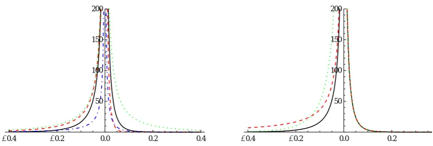
Fig. 1 left panel: Lévy measure of a VG process for the following four sets of

parame-ters q = -0.29, s =0.19, n =0.25 (solid line); q = -0.99, s =0.19, n =0.25, (dashed); q = -0.29, s =0.99, n = 0.25 (dotted) and q = -0.29, s =0.19, n = 0.95 (dot-dashed); right panel: The LG Lévy measure for l =1, and the following three sets of parameters d0 = -0.11, d1 =0.04, a0 = a1=3.99 (solid line); d0= -1.13, d1 =0.04,

a0= a1=3.99 (dashed); and d0= -0.11, d1 =0.04, a0= 11.98, a1=3.99 (dotted);

As known, (see Proposition 3.18 of Cont and Tankov 2004) the exponent of a (univariate) Lévy process with characteristic triplet, g, A,k is a martingale if and only if, 

x¥1‰

x_k_„x_{< ¶ and}

(15)

A

2 + g +-¶ +¶

‰x_-1-x

x§1kL G„x=0.

Based on this result, Propositions 4 and 5 establish the conditions for the exponent of an LG process to be a martingale a property which is important in financial applications.

Proposition 4. Given n¥1, ai>0, di∫0, i=0, …, n, _x¥1‰xkL G„x< ¶ if

l >maxiœD+di.

Proof. It can be directly verified, substituting kL G„x from (12) that, for x>0,

(16) 

x¥1

‰x_kL G_„x_{= } iœD+



1 +¶_a

iexp-xldi -1

x „x.

We have that,



1 +¶_a

iexp-xldi -1

x „x=¶

aiE1ldi -1< ¶, if l > di diverges, otherwise,

[image:18.595.106.532.77.221.2]

Similarly, it can be verified that, for x<0, we have that

 x¥1

‰x_kL G_„x_{= } iœ

D-

1 +¶_a

iexp-x ldi +1

x „x= -

iœ

D-aiEildi -1< ¶,

where Eild_i -1 denotes the Exponential Integral function (defined in section 5.1.2 of Abramowitz and Stegun 1972), evaluated at ldi -1<0, from where it can be seen that, in order for the sum in (16) to converge, no additional conditions on the parameters l and dineed to be imposed. á

Proposition 5. There exist n¥1, ai>0, di∫0, i=0, …, n and l >maxiœD+di such

that, the expLGt;d,a, l, n is a martingale, i.e.,

(17) 

-¶ +¶

‰x_-1_kL G_„x_=0.

Proof. Clearly, the necessary condition, l >maxiœD+di, established by Lemma 4, can

be met for arbitrary positive real parameters di, iœD+. The necessary and sufficient

condition (17), for expLGt;d, a, l, n to be a martingale, directly follows from (15) and (14), noting that, for a LG process, A=0. For the integral in (17), we have

(18) 

-¶ +¶

‰x_-1_kL G_„x₌



-¶ 0

x

j=0

¶ _xj

j+1! _i_œD-ai ‰-l

x

di

x „x+0 +¶

x

j=0

¶ _xj

j+1! _i_œD+ai ‰-l

x

di

x „x=

 iœD+

ai j=0

¶



0

+¶ _xj j+1! ‰

-lx

di „x- 

iœ D-ai

j=0

¶



-¶ 0 _xj

j+1! ‰

l x

di „x=

 iœD+

ai j=0

¶ _d

i l

j+1 ₁

j+1- 

iœ D-ai

j=0

¶

-1j di l

j+1 ₁

j+1 =

-_

iœD+

ailn 1 -di

l -_i_œD-ailn 1+ di

l ,

where ln1-d_li is well defined, given that, l >maxiœD+di, as required by Proposition 4. It is not difficult to see that the right-hand side of (18) vanishes if n¥1, the sets D

-and D+ have equal cardinality and if

-ai-ln 1+ di-

l = ai+ln 1 -d_i+

l ,

(19) -ai- = ai+, di-=

-d_i+l d_i+- l

andl >maxiœD+di.

Hence, for a fixed n¥1, one can always chose a set di, iœD+ and select values, l,

di-, i-œD-, and ai, i œ I, according to (19), so that (18) vanishes, which completes the proof of the asserted existence. á

Remark 1. Propositions 4 and 5 state that, it is possible to select the parameters n, d, a

and l of a LG process in such a way that the exponent, expLGt;d, a, l, n, is a martin-gale. However, it is not difficult to see from the LG representation, (3), of a VG process that, there does not exist a set of VG parameters, q,s,n for which expV Gt;q,s,n is a martingale.

We conclude this section by briefly indicating that the (univariate) LG process can be used for modelling asset price dynamics. Define the (risk-neutral) asset price process,

St as

(20)

St=S0expr-q+ wt+LGt;d,a,l,n

where r - the (constant) risk-free rate, q - the dividend yield, and the constant w is cho-sen so that St=S0expr-qt, i.e.

(21)

w = _

iœD+

ailog 1 -di

l +_i_œD-ailog 1+ di

l

which follows from Proposition 5. We therefore require l >max_iœD+di. Note that, in the special case of the VGt;q,s, n process (21) yields

w = 1

n log 1 q n -s2_n

2 ,

where 1> q

2_+2s2_{n +q}

2 n (which implies 1>q + s

2₂_n).

The model given by (20) can be used in (exotic) option pricing and pricing participating life insurance contracts. Due to volume limitations, details of how this is done are out-side the scope of this paper and will appear elsewhere.

3 Multivariate LG processes

Definition 2. Define the multivariate LG process, LGt=LG1t, …, LGst', s¥1

as

(22) LG₁t= d_1,0G₀t;a₀, l+...+ d_1,nGnt;a_n,l

ª

LGst= d_s,0G₀t;a₀,l+...+ d_s,nGnt;a_n, l,

where dj= d1,j, ..., ds,j', djœs, j=0, ...,n, are pairwise distinct, n¥s, l >0,

a =a0, ...,an, aj>0, j=0, ...,n and Gjt;aj,l, j=0, ..., n are independent

Gamma processes defined on a probability space W,, .

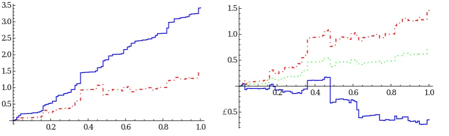
Multivariate LG processes are illustrated graphically in Fig. 2 where we have simulated sample paths from two and three dimensional LG processes with coordinates

LG1t= -5G0t; 1, 20-2G1t; 10, 20+2G2t; 30, 20,

LG2t= -2G0t; 1, 20+1G1t; 10, 20+2G2t; 30, 20,

with mLG1=1.75, nLG1=0.46, mLG2=3.40, nLG2 =0.34 and

LG1t= -5G0t; 1, 20-2G1t; 10, 20+2G2t; 30, 20,

LG₂t= -6G₀t; 1, 20-3G₁t; 10, 20+1G₂t; 30, 20,

LG₃t= -3G₀t; 1, 20-1G₁t; 10, 20+1G₂t; 30, 20,

with m_LG1=1.75, n_LG1=0.46, m_LG2 = -0.3, n_LG2=0.39, and m_LG3=0.85, n_LG3=0.12

respectively, where mLGi,nLGi i=1, 2, 3 are the corresponding (marginal) mean and

variance rates. As can be seen from Fig. 2 all coordinates jump together, which is a consequence of the fact that for a fixed t, a multivariate LG process represents a linear transformation of a set of Gamma processes, in this case these are G₀t; 1, 20,

G1t; 10, 20 and G2t; 30, 20. It should also be noted that simulation of a multivariate

LG is straightforward since it requires simulating Gamma sample paths which is done very efficiently, applying the Dirichlet bridge sampling method, recently proposed by Kaishev and Dimitrova (2009).

0.2 0.4 0.6 0.8 1.0 0.5

1.0 1.5 2.0 2.5 3.0 3.5

0.2 0.4 0.6 0.8 1.0

-0.5 0.5 1.0 1.5

[image:21.595.100.539.578.711.2]

Before proceeding further, we will need to introduce the following notation. For a given set AÕs, Ax, A, volsA, dimA denotes the indicator function, the closed convex

hull, the s-dimensional Lebesgue measure and the dimension respectively. By x, y, z, … we denote elements (vectors) in the Euclidean space s _s¥1_{, i.e., x=}_x

1, …, xs'

where, ', means transposition and we use subscripts to index vectors, i.e., x_j=x_1,j, …, x_s,j', j=0, 1, …. We denote by xÿy=_is₌₁x_iy_i the inner product of x, yœs.

3.1 Distributional properties

In what follows, we study distributional properties of multivariate LG processes and establish their relation to multivariate splines. For the purpose we will need to introduce multivariate B-splines, known also as simplex splines. A simplex spline is a multivariate version of the univariate polynomial B-spline defined in Section 2.1. Simplex splines, were first introduced by De Boor (1976) as follows.

Definition 3. (De Boor 1976). Let =y0, ..., yr be any r-simplex in r,

r_=s_är-s_{, such that y}

j s= d_j, j=0, ...,r, i.e., the first s coordinates of y_j agree

with the vector d_jœs_{, s¥1. The multivariate (simplex) spline M}_x;d

0, ..., dr is

defined as

Mx;d₀, ...,dr=vol_r-suœ:u s = x volr.

Note that Definition 3 allows for coalescent knots, d₀, ..., d_r of which say,

n + 1 < r+1 knots, d0, ..., dn may be distinct with corresponding multiplicities a0, ..., an. If there are d0, ..., dn pairwise distinct knots with multiplicities a0, ..., an,

Mx;d₀, ..., dr, will be alternatively denoted as M x;d₀,

a0,

..., d_n

...,an

,vœs _{and also as}

M x1, ..., xs;d0, a0,

..., dn

...,an

.

The simplex spline, Mx;d0, ...,dr is a piecewise polynomial of total degree not exceed

ing r-s with r-s-1 continuous derivatives when the knots, d0, ...,dr are in general position. The knots, d₀, ..., d_r, are said to be in general position if for j=1, ...,s and for arbitrary, different indexes 0§i₁, ..., i_j+1§r, we have

det

1 d1,i1 ... dj,i1

1 d1,i2 ... dj,i2

ª ª ... ª

1 d1,ij+1 ... dj,ij+1

∫0.

(23)

Mx;d₀, ..., dr= r

r-s 

j=0 r

ljMx;d0, ..., dj-1,dj+1, ..., dr,

whenever r>s and the numbers, l_jœ, are such that, x=jr₌₀l_jd_j, jr₌₀l_j=1.

For further properties of simplex splines see e.g., Neamtu (2001), Cohen et al. (2001) and Prautzsch et al. (2002).

We will now recall that simplex splines have a nice probabilistic interpretation estab-lished independently by Karlin et al. (1986) and Ignatov and Kaishev (1985, 1989) which we will exploit in studying the properties of multivariate LG processes.Given the set of knots D =d0, ...,dr, dj= d1,j, ..., ds,j', djœs, j=0, ..., r, consider the random vector B=B1, ..., Bs', defined by

(24) B=d₀q₀+...+d_rq_r,

with coordinates Bi= di,0q0+...+ di,rqr, i=1, ..., s, where the random vector

q=q0, ...,qr', is Dirichlet distributed with parameters a =1, ..., 1, i.e.

q0, ..., qrœ1.

It will be convenient to view the vectors d0, ...,dr as points in s, s¥1. Note that in (24), we allow some of the points d₀, ...,d_n to coalesce. Let us assume that only n+1 of them are pairwise distinct, say d0, ...,dn, each repeated with multiplicity a0, ..., an, a0+...+ an=r+1. Then, given the set of distinct knot parameters, D =d0, ..., dr,

following a well known property of the Dirichlet distribution (see e.g., Wilks 1962), the random vector B=B₁, ..., Bs', defined by (24), can be rewritten as

(25) B=d0q0+...+dnqn,

with coordinates Bi= di,0q0+...+ di,nqn, i=1, ..., s, where the random vector

q=q0, ...,qn', is Dirichlet distributed with parameters a =a0, ..., an, i.e.,

q0, ..., qnœa0, ...,an.

Assume also that the parameters a, D, r, and n, are such that the distribution of the

linear transformation B and its marginal distributions exist and are non-degenerate. Denote by fBx the density of B. The following result establishes the probabilistic interpretation of simplex splines.

Theorem 2. (Ignatov and Kaishev 1985, 1989). Let d₀, ...,d_n be fixed pairwise distinct

vectors in s_{, n¥s, with dimension dim}_d

M x;d0, a0,

..., dn

...,an

with knots d0, ..., dn having (integer) multiplicities, a0, ..., an, a0+...+ an=r+1. As in the univariate case, the Dirichlet parameters a0, ..., an, may in general take real values. In this case the density, f_Bx, has been viewed by Ignatov and Kaishev (1987, 1988) as a multivariate generalized B-spline i.e., as multivariate Dirichlet spline. Indepen-dently, Karlin et al. (1986) have also considered similar generalization of multivariate simplex splines. For some further properties of multivariate Dirichlet splines see Karlin et al. (1986), Ignatov and Kaishev (1987, 1988) and Neuman (1994).

The following proposition gives for fixed t>0 an expression for the joint density of the multivariate LG process in terms of multivariate Dirichlet splines.

Proposition 6. Let d0, …, dn, djœs, n¥s, be pairwise distinct and let

dimd0, …, dn=s, then the density of LG is

(26)

fLGx1, ..., xs=



0

+¶ _la0+...+ant

Ga0+...+ ant

ya0+...+ant-s+1‰-ly_M

g

x1

y, ..., xs

y;ad00t,,

...,

...,

dn

ant

„y,

where Gÿ is the gamma function and M_g x1

y, ..., xs

y; d0,

a0t,

...,

...,

dn

ant

is a multivariate

Dirich-let spline with knots D =d₀, …, dn, of multiplicities a₀t, ...a_nt.

Proof. We have that the multivariate LG process can be represented as

(27) LGt;D, a, l, n= Btä Gt

where Bt is defined as in (25) and has a joint density fBtx, which, by Theorem 2, coincides with a generalized B-spline, and where the random variable, Gt=_in₌₀Git;ai, l, independent of Bt, is gamma distributed with parameters a0+...+ ant and l. Thus, we have

fLGx₁, ..., xs= ∑

∑x₁…∑x_sPB1täGt§x1, …, BstäGt§xs

= ∑

∑x₁…∑x_sP B1t§

x1

Gt, …, Bst§ xs Gt

= _

0

+¶ _∑

∑x₁…∑x_sP B1t§

x1

y, …, Bst§

xs

= _

0 +¶

fBt

x1

y , …,

xs

y fGty

1

ys „y.

The result now follows, in view of (7) and noting that, by Theorem 2, fBtx_y1, …, xs

y

coincides with a multivariate Dirichlet spline, M_g x1

y, ..., xs

y; d0,

a0t,

...,

...,

dn

ant

. á

In case a_it, i=0, ...,n, are integers then Mgÿ is a classical multivariate polynomial

simplex spline, given by Definition 3 and its evaluation can be successfully performed using e.g. Michelli's recurrence (23). When the multiplicities a_it, i=0, ..., n are non-integer, to the best of our knowledge, the evaluation of multivariate Dirichlet splines has not been sufficiently explored. Recurrence formulas for the moments of multivariate Dirichlet splines and simplex splines have been established by Neuman (1994).

In order to provide some insight into the dependence properties of multivariate LG processes, next we give its underlying copula.

Proposition 7. The copula CLGu1, ...,us, is given as

(28)

CLGu1, ...,us=



-¶

FLG1 -1_u

1

…

-¶

FLGs

-1_u

s



0

+¶ _la0+...+ant

Ga0+...+ ant

ya0+...+ant-s+1‰-ly

Mg

x₁

y , ..., xs

y;da00t,,

...,

...,

dn

ant

„y„xs…„x1,

where u_iœ0, 1, and

F_LGix=

-¶

x 

0

+¶ _la0+...+ant

Ga0+...+ ant

ya0+...+ant-2‰-ly_M

g

x

y;d_aj,0,

0t,

...,

...,

dj,n

ant

„y„z,

i=1, ...s.

Proof. Expression (28) follows from the Sklar's Theorem and expressions (26) and (6).á

Let us note that the LG copula CLGu1, ..., us is related to the (new) class of the

The next proposition gives the characteristic function of a multivariate LG process, which will be needed in order to develop a method of moments for estimating the LG parameters.

Proposition 8. The characteristic function, fz, of the multivariate LG process,

LGt=LG₁t, …, LGst' given by Definition 2 is

(29) fLGz=

j=0

n _l

l -idjÿ z

aj

,

where dj=d1,j, …, ds,j' œs, j=0, …, n , z=z1, …, zs'œs and l >0 .

Proof. From Definition 2, for fixed t, say t=1 and z=z1, …, zs'œs, it is directly

seen that the characteristic function

fLGz=‰izÿLGt=‰

in_j=0djÿz Gjt;aj,l

= _

j=0 n

‰idjÿz Gjt;aj,l=

j=0

n _l

l -id_jÿ z

aj

,

which completes the proof of the asserted expression for f_LGz. á

In order to develop a method of moments for estimating the LG parameters, we will give here the moment generating function (mgf)

M_LGz=‰zÿLGt_=

j=0

n _l

l - djÿ z

aj

,

and the cumulant generating function (cgf)

(30)

KLGz=logMLGz=

j=0 n

-ajlog 1 -1 l djÿ z

of the LG random vector.

3.2 LG parameter estimation: method of moments